Migration of a moonlet in a ring of solid particles :
Theory and application to Saturn’s propellers.
Abstract
Hundred meter sized objects have been identified by the Cassini spacecraft in Saturn’s A ring through the so-called “propeller” features they create in the ring. These moonlets should migrate, due to their gravitational interaction with the ring ; in fact, some orbital variation have been detected. The standard theory of type I migration of planets in protoplanetary disks can’t be applied to the ring system, as it is pressureless. Thus, we compute the differential torque felt by a moonlet embedded in a two-dimensional disk of solid particles, with flat surface density profile, both analytically and numerically. We find that the corresponding migration rate is too small to explain the observed variations of the propeller’s orbit in Saturn’s A-ring.
However, local density fluctuations (due to gravity wakes in the marginally gravitationally stable A-ring) may exert a stochastic torque on a moonlet. Our simulations show that this torque can be large enough to account for the observations, depending on the parameters of the rings. We find that on time scales of several years the migration of propellers is likely to be dominated by stochastic effects (while the former, non-stochastic migration dominates after years). In that case, the migration rates provided by observations so far suggests that the surface density of the A ring should be of the order of kg m-2. The age of the propellers shouldn’t exceed to million years, depending on the dominant migration regime.
Keywords:
planets and satellites: dynamical evolution and stability — planets and satellites: individual (Saturn) — planets and satellites: rings — planet-–disk interactionsI Introduction
The theory of disk-satellite interactions has for the most part been developed after Voyager’s encounter with Saturn. The satellites that orbit beyond the outer edge of the rings perturb the dynamics of the particles composing the rings. This leads to an exchange of angular momentum between the rings and the satellites, and to the formation of density waves in the rings. Lin and Papaloizou [23] and Goldreich and Tremaine [16], Goldreich and Tremaine [17] have calculated, using two different methods, the total torque exerted by a satellite on a disk interior (or exterior) to its orbit. This torque is called the one-sided Lindblad torque, because it can be computed as the sum of the torques exerted at Lindblad resonances with the secondary body. In the lowest order, local approximation, the inner and outer torques are equal and opposite : the torque exerted by a satellite on a disk located inside its orbit is negative, with the same absolute value as the positive torque exerted on a disk located outside the orbit.
Reciprocally, a disk exerts a torque on the secondary body. When the strictly local approximation is relaxed, the inner and outer torques are not exactly equal and opposite [43]. Their sum, called the differential Lindblad torque, is generally negative. As a consequence, the orbital angular momentum of a body embedded in a disk decreases, and so does its semi-major axis (on circular Keplerian orbits, the orbital angular momentum is proportional to the square root of the semi-major axis). This is planetary migration of type I [45]. So far, this phenomenon has been mainly studied in the frame of planets embedded in protoplanetary gaseous disks [see 28, for a review].
The Cassini spacecraft has been orbiting the Saturnian ring system since 2004, offering the possibility to observe the coupled evolution of the ring system and the satellites. Due to short orbital timescales (1 year is equivalent to about 700 orbits of the A ring) it may be possible to observe the exchange of angular momentum between the two systems. One of the most striking discoveries of the Cassini spacecraft is the observation of propeller shaped features in the A ring (located between and km from Saturn), with longitudinal extent about km [40, 39, 37]. They are most probably caused by the presence of moonlets about hundred meters in size, embedded in the ring, and scattering ring particles [36]. As they are embedded in the ring, these small bodies should exchange angular momentum with the ring, and migrate [10]. This migration could be detected by Cassini observations through the cumulative lag, or advance with time of the orbital longitude induced by a small variation of the semi-major axis and the angular velocity (), offering for the first time the possibility to confront directly the planetary migration theory with observations, and to give insights and constrains on the physical properties of the rings and of the moonlets.
In this paper, we address the question of the theoretical migration rate of these propellers, using both numerical and analytical approaches. The theory is then confronted to observations. In Sect. II, we review the standard theory of type I migration ; the differences between migration in protoplanetary disks and in Saturn’s rings are explained, showing the need for a new calculation of the migration rate of embedded moonlets. This rate is given in Sect. III for an homogeneous, axisymmetric disk with a flat surface density profile, as a result of numerical computation in Sect. III.1, and analytical calculation in Sect. III.2. In Sect. IV, we consider the effect of density fluctuations in the rings, in particular the role of short-lived gravitating clumps, also called gravity wakes, which are known to be numerous in the A ring [9]. We then conclude in Sect. V on what our model tells us on the properties of the rings, given the observed migration rates.
II Review of Type I migration and the differential Lindblad torque
In protoplanetary gaseous disks, the perturbation caused by a terrestrial planet leads to the formation of a one armed spiral density wave, leading the planet in the inner disk, and trailing behind the planet in the outer disk. This wave is pressure supported and generally called the wake, but it has nothing to do with the gravity wakes mentioned above : the latter are local features, while the planet wake spirals through the whole disk. The planet wake carries angular momentum, so that the angular momentum given by the planet to the disk is not deposited locally [e.g. 11, Appendix C]. Therefore, the disk profile is hardly modified in this linear regime. Still, the negative torque exerted by the outer disk on the planet through the wake is larger in absolute value than the positive torque from the inner disk. Without going into the details [45, for which the reader is refereed to], the main reason the outer disk wins over the inner disk lies in pressure effects : from the dispersion equation of a pressure supported wave, one finds that the location where the wave with azimuthal mode number , corresponding to the th Lindblad resonance with the planet, is launched, is not exactly the location of the resonance given by Kepler’s laws. The shift is not symmetrical with respect to the planet position for inner and outer resonances, but favors the outer ones. As a consequence, the planet feels a negative total torque, called the differential Lindblad toque, and given by Tanaka et al. [38] :
| (1) |
where the index refers to the planet, being the radius of its orbit and its angular velocity, is the planet to primary mass ratio, is the surface density of the disk in the neighborhood of the planetary orbit. Finally, is the aspect ratio of the disk, being the ratio between its scale height and the distance to the central body, being proportional to the square root of the gas pressure. In a typical protoplanetary disk, . The numerical coefficient is given by , where is the index of the power law of the density profile : .
This result is robust. In particular, the value of the negative torque is almost independent on the slope of the density profile . This is due to the so-called pressure buffer : the resonances are shifted when the density gradient varies [45]. If the disk were pressureless, then the expression of would be completely different. Also, the aspect ratio in Eq. (1) appears because doesn’t converge towards when tends to infinity, but towards , due to pressure effects. To sum up, the gas pressure plays a fundamental role in type I migration.
It should be mentioned for completeness that, in addition to the differential Lindblad torque discussed above, the horseshoe drag – exerted on the planet by the gas on horseshoe orbits around the planetary orbit – plays a significant role in type I migration [44, 24, 3, 20, 27, 26, see e.g.].
In contrast to gaseous protoplanetary disks, pressure effects in Saturn’s rings are not important. The aspect ratio is of the order of . The spiral density waves that are observed in the A ring are gravity supported, not pressure supported. Thus, the standard theory of type I migration does not apply. In particular, the spiral planet wake doesn’t appear. The interaction of the moonlet responsible for the propeller structure with the disk is observed to take place within a few hundred kilometers. Resonances with are located within this distance and should play a significant role. However, in the standard type I migration the important resonances have . Therefore, Eq. (1) can’t be directly applied to a moonlet in Saturn’s rings. A new approach is needed, adapted to the two main characteristics of the problem : the fact that the rings are made of solid particles, and the fact that the interaction is taking place very close to the moonlet.
III The ring-moonlet interaction
In this section, we compute the interaction between a moonlet and a ring test particle. In this analysis, the gravity of the other ring particles is neglected. This leads to the torque exerted on the moonlet by an initially unperturbed, homogeneous ring. In subsection III.1, the computation is performed numerically. In subsection III.2, it is derived analytically. Both results are in agreement, and a corresponding migration rate for the moonlet is given and discussed in subsection III.3.
From now on, denotes the mass of the moonlet (and not anymore the order of a resonance). The moonlet, has a circular orbit of radius around the central planet of mass . The gravitational potential due to the moonlet is . The radial and azimuthal components of the equation of motion of a ring particle in two dimensional cylindrical polar coordinates are
| (2) |
| (3) |
The angular velocity of the moonlet is . Let be the radius of the initially circular orbit of a test particle and its angular velocity. We note is the impact parameter, and the normalized impact parameter, where is the Hill radius of the moonlet.
III.1 Numerical computation of the ring moonlet interaction
In this section, the numerical integration of the above equations of motion is performed, in order to find the trajectories of ring particles in the presence of a perturbing moonlet in the frame corotating with the moonlet. To measure the tiny asymmetry between the inner and the outer part of the ring, the full equations are integrated, without linearization or simplification. A Bulirsch-Stoer algorithm [31] is used, and a Taylor expansion is performed in the code when necessary to subtract accurately large numbers, in order to achieve machine double precision (). We have checked that the Jacobi constant is conserved to this precision along the trajectories. Examples of obtained trajectories are given in Fig. 1.

It is well known within the framework of the restricted 3-body problem that if is small enough, the test particle has a horseshoe shaped orbit, while if is larger than , the test particle is circulating, and scattered into an eccentric orbit. This can be seen in Fig. 1. We perform many numerical integrations with various in the case of a moonlet of mass , starting the particle at an azimuth (where the moonlet is at ). This angle is large enough so that at this location the influence of the moonlet is negligible and the orbital parameters of the test particle are not disturbed, as will be checked later. We find that the horseshoe regime occurs for , and the scattered regime occurs for . For , however, the trajectory approaches the center of the moonlet to within a distance smaller than . In that case, if one assumes the moonlet is a point mass, the test particle eventually leaves the Hill sphere, either on a horseshoe or a circulating trajectory, but the outcome changes several times with increasing . In the case we are concerned about here, the moonlet most likely almost fills its Roche lobe, and therefore we stop the integration of the trajectory as soon as the distance between the test particle and the moonlet is less than , assuming a collision.
The specific orbital angular momentum of the test particles is computed along the trajectories. Angular momentum is exchanged during the close encounter with the moonlet. For , the test particle is scattered onto an eccentric orbit of larger angular momentum than initially, which results in a gain in angular momentum. The variation of orbital angular momentum along the trajectory is shown in the bottom panel of Fig. 2 for the case , where the top panel is the trajectory. The difference in angular momentum between the initial circular orbit at and the end of the integration, when again, is noted . In the figure, only the interval is displayed, for convenience. Most of the exchange of angular momentum occurs when .
Figure 3 shows (top thick curve) as a function of , in units of the specific angular momentum of the moonlet . For , the horseshoe trajectory corresponds to a U-turn towards the central planet, and to a loss of angular momentum for the test particle. More precisely, as for circular orbits , one expects for such a U-turn ; this is indeed the case for . In the case where the test particle collides with the moonlet, we assume that it gives all its orbital angular momentum to the moonlet : , so that . This also appears in Fig. 3. The opposite holds for .

Computing as a function of to numerical precision enables us to also compute the difference between the inner and outer disk : . This quantity is small with respect to , but nonetheless well determined and converged in our simulations : is constant after the encounter to a precision better than for all . This validates our choice of . In Fig. 3, the bottom thick dashed curve shows in the same scale as . We see that for all and that , with
| (4) |
for circulating trajectories, and
for horseshoe orbits. In the following subsection, the empirically found Eq. (4) is derived analytically and justified.

III.2 Analytic model for the ring moonlet interaction
In this section, we consider only circulating trajectories. Developing to second order the exchange of angular momentum during an encounter with the moonlet , we can find the asymmetry .
III.2.1 Solution for the perturbed moonlet orbit
Let us start again from Eq. (2) and (3). The ring particle is assumed to be on an unperturbed circular orbit of radius It orbits with angular velocity such that , where without loss of generality we have defined the origin of time to be when the particle is at . Under the perturbation induced by , the particle moves to and , where and are assumed to be small. Linearizing Eq. (2) and (3) about the circular orbit state, we obtain equations for and in the form
| (5) |
| (6) |
Here the subscript denotes evaluation on the unperturbed particle orbit.
We suppose that the perturbation is induced by a moonlet of mass that is on a circular orbit of radius and has an angular velocity Then its azimuthal coordinate with being a constant. The perturbing potential
| (7) |
becomes a function of time through substituting therein.
III.2.2 Solution of the linearized equations
To solve Eq. (10), we note that the perturbing potential Eq. (7) evaluated on the unperturbed orbits is a periodic function of time with period Thus we should look for a periodic response. In order to do this we have to introduce a small frictional term into Eq. (10) to enable transients to decay and a net torque on the moonlet to be set up. When the frictional term is small it is expected that the resulting torque should not depend on it [17, e.g.]. Hence we add a frictional term to the left hand side of Eq. (10), where is a small constant parameter so that it now reads
| (11) |
As the potential is periodic in time we can adopt a Fourier series of the form
| (12) |
where it is implicit that the real parts of such complex expressions is to be taken, and
| (13) |
The periodic solution of Eq. (11) is now readily written down as
| (14) |
We may write this in terms of a Green’s function defined through
| (15) |
Then the solution for may be written
| (16) |
Note that as the orbit of a ring particle relative to the planet is periodic, the solution given by Eq. (16) includes the effects of infinite numbers of repeating encounters. However, we wish to consider the case when dissipative effects, although weak, are strong enough to recircularize orbits between encounters in which case they will be independent of each other. This condition requires that This is equivalent to requiring that the damping time scale be short compared to the relative orbital period between moonlet and ring particle. On account of the length scale of the encounters of interest being comparable to the Hill radius of the moonlet, this is much longer than the orbital period itself, so that we may adopt the ordering
| (17) |
In order to make use of the above ordering we write down the form of the Green’s function derived in the appendix (see Eq. (A7) ) valid for
| (18) |
where The function is defined elsewhere through its periodicity with period Making use of the inequality Eq. (17) we may replace the Green’s function Eq. (18) by the simple expression
| (19) |
Then the solution Eq. (16) gives
| (20) |
where
| (21) |
and
| (22) |
To make use of the above expressions, we consider the situation when the ring particle has a close encounter with the moonlet at time thus we take (we note that a non zero can be dealt with by rotating the coordinate system and shifting the origin of time). The source term is then expected to be highly peaked around and almost all of the contributions to the above integrals will occur for Furthermore, during this dynamical interaction, dissipation will be negligible. Thus, if we are interested in times after the main interaction, but before significant dissipation takes place, we may set and extend the limits of the integration to However, in practice one may have to apply a cut off to the potential at large distances from the moonlet in order to do that (see below). But this should not matter if the important interaction occurs when the moonlet and ring particle are close.
Then we simply have
| (23) |
and
| (24) |
Thus and are constants representing epicyclic oscillation amplitudes induced after the close approach of the ring particle to the moonlet.
We remark that the approximations made in obtaining Eq. (23) and Eq. (24) relate to how dissipation is treated. There has been no assumption that the particle trajectories are symmetric on opposite sides of the moonlet so that curvature effects remain fully incorporated during particle moonlet encounters. When dissipation is negligible during the encounter, then immediately afterward an epicyclic oscillation is established. The assumption that dissipation circularizes orbits between encounters implies that we should consider approaching ring particles to be on circular orbits. The above discussion indicates that errors associated with this assumption are exponentially small.
III.2.3 Angular momentum transfer
For the set up considered here, symmetry considerations imply that is an even function of time (see below), so that . The generation of the epicyclic oscillation is associated with an angular momentum transfer between the moonlet and particle. To find this we firstly note that
| (25) |
where and are the post encounter semi-major axis and eccentricity of the particle. We also note that the Jacobi constant implies that the change of the particle orbital energy and angular momentum are related by . This can be used to eliminate in Eq. (25) after which may be found correct to second order in with the result that . This in turn may be simply determined after evaluating . Note that for particles interior to the moonlet which have and conversely for particles orbiting exterior to the moonlet.
III.2.4 Development of the perturbing potential
We now consider
| (26) |
We begin by recalling that
| (27) |
In order to evaluate the Fourier transform as specified by Eq. (23), which was derived under the assumption that the interaction occurs only near closest approach, we must truncate the potential at large As the encounter takes place over a time this can be achieved by replacing in Eq. (27) by Note that a dimensionless estimate of the error involved is of order where is the Hill radius of the moonlet. This is small enough that the leading order asymmetry in the angular momentum transferred to orbits with the same impact parameter on either side of the disk can be estimated.
As the first stage in evaluating the Fourier transform of specified in Eq. (23) that gives the epicyclic amplitude, we evaluate
| (28) |
This can also be expressed as
| (29) |
where and denotes the modified Bessel function of the second kind of order
III.2.5 Total angular momentum exchange
We may now use the above expression together with Eq. (26) to evaluate the epicyclic amplitude Eq. (23) (noting that the radial derivative is with respect to with other quantities held fixed) so obtaining
| (30) |
The associated angular momentum exchanged is then given by
| (31) |
In a strictly local approximation under which the inner and outer sides are symmetric, the contributions from orbits equidistant from the moonlet would cancel, leaving the net result to be determined by the surface density profile. However, although we have assumed the interactions are local, we did not assume symmetry between the exterior and interior orbits. Accordingly we evaluate the difference in the magnitude of evaluated from orbits equidistant from the moonlet : . The leading order contribution to is symmetric in . The lowest order contribution is antisymmetric and accordingly leads to cancellation between the two sides. We make use of the expansions , and together with standard properties of Bessel functions to write
| (32) |
where
| (33) |
The first order term of Eq. (32) was already given by Goldreich and Tremaine [17]. It is plotted as a straight green dashed line in Fig. 3. Our expansion to second order enables us to go further, and to give the expression of the magnitude of the asymmetry between the two sides of the disk :
| (34) |
It is such that for an orbit with a given impact parameter, the angular momentum exchanged in the outer disk is the larger.
In the case studied numerically, we had , so that . Then, Eq. (34) remarkably agrees with the numerical fit Eq. (4). The light blue dot-dashed curve in Fig. 3 displays .
In the context of the above, we note that approximations made in obtaining equation Eq. (31) such as effectively starting and truncating the interaction at some finite though large distance from the moonlet could conceivably lead to changes comparable to those given by Eq. (34). However, such changes are again approximately symmetric for trajectories on both sides of the moonlet and thus approximately cancel so we do not expect such effects to significantly alter Eq. (34).
III.3 Migration rate and discussion
If the surface density of ring particles is , the total rate of angular momentum transferred to the moonlet is
| (35) |
where the integral is taken over the disk. The particles exterior to the moonlet contribute negatively while those interior contribute positively. The cumulative torque exerted by the moonlet on the region of the ring located within a distance to its orbit reads then :
| (36) |
The normalized cumulative torque
is plotted in Fig. 4. The proportionality to is obvious ; that is numerically verified for , and has been already found analytically by Ward [44] for the horseshoe drag in a similar context.
Most of the total torque comes from scattered, circulating particles, in particular the ones with smallest impact parameter . This makes the total torque sensitive to the physical size of the moonlet (taken as here), as some particles colliding with the moonlet could be circulating if it were smaller.
The role of the horseshoe drag appears to be non negligible, amounting to
. The expression of Ward [44] for the torque arising from material executing horseshoe turns, called the horseshoe drag, is for a Keplerian disk with flat density profile :
| (37) |
where is the half-width of the horseshoe region. In our case, , which gives . The agreement is good because Ward’s analysis is based only on geometrical effects and angular momentum variation in a Keplerian disk, without any pressure effect. Therefore, it also applies in Saturn’s ring. We remark that taking in Eq. (37) gives a perfect match with what we find numerically for the total horseshoe drag.

In conclusion, from Fig. 4, the total torque felt by a moonlet of mass on a circular orbit of radius around a planet of mass can be written as
| (38) |
Note that to get the same dependency of the type I torque in the parameters of the system, one has to assume in Eq. (1) ; however, in a protoplanetary disk, is fixed and independent of the mass of the secondary body, so that this proportionality would not be justified.
The torque is related to the migration speed through Hence we deduce that
| (39) |
The migration rate is here proportional to the mass of the moonlet to the power , in contrast to standard type I migration where . A numerical application to the case of an kg moonlet in orbit in the A-ring of density kg m-2 at km from Saturn gives m yr-1. Increasing the mass by two orders of magnitude to correspond to a radius of m speeds up the migration rate by a factor of only to m yr-1.
After time , a migrating propeller will be shifted longitudinally with respect to a corresponding non migrating one by a distance . For the above parameters, this gives m. A shift of this magnitude is potentially detectable on a timescale of a year to a few years (30 and note also 5). Actually, migration of propellers has already been detected [5, 41]. During one time period of nearly a year, a particular propeller has been seen moving outward at a rate of m yr-1 ; and during a later similar time period, the same propeller has been seen moving inward at a rate of m yr-1 [41, and personal communication].
These observations are not compatible with the above theory. But we recall that the process of migration of a moonlet described above assumed a smooth particle disk with constant surface density. Here we note that there are features and mechanisms that might produce a significantly faster migration rate, possibly in both directions inward and outward, and non constant in time. One can first think of a radial density gradient : as there is no pressure buffer here, this would directly affect the balance between the torques from the inner and outer parts of the ring. This would also affect the torque from the horseshoe region, which could turn positive. However, if the migration is governed by the gradient of some quantity, it seems likely that the moonlet would have approached an extremum in that quantity, and thus should have attained a migration rate comparable to that estimated for a constant surface density.
Another possibility resulting in the moonlet migrating faster than what the previous calculation indicates, and possibly outward, is a runaway migration in a planetesimals disk [19, 21, for a review], similar to the type III migration of planets in protoplanetary disks [25]. In this regime, the migration of the moonlet in the disk leads to a positive feedback on its migration rate, because of the material of the inner (resp. outer) disk making horseshoe U-turns to the outer (resp. inner) disk. This speeds up the migration, possibly leading to a runaway. However, this leads inevitably to an asymmetry in the horseshoe region, while the propeller structures observed are rather symmetrical.
Finally, the A-ring of Saturn is not homogeneous. It is close to gravitational instability, which should lead to the formation of gravity wakes and density fluctuations. The effect of these density fluctuations on the moonlet is studied in next section.
IV The role of density fluctuations and resulting stochastic migration
The analytic calculations and numerical simulations in the previous chapters assume an inflow of particles on circular orbits only perturbed by the nearby moonlet. However, we know that Saturn’s A ring is marginally gravitationally stable [13]. The Toomre parameter [42], which is a measure of the importance of self-gravity, is expected to be of the order of , indicating that the ring particles’ mutual gravity is indeed a strong effect. It leads to the regular formation and dispersion of gravity wakes, which are local density enhancements elongated in parallel directions by the Keplerian shear. Those over-densities give rise to stochastic forces which act on the embedded moonlet.
A very similar effect is expected to occur in protoplanetary disks. These disks are thought to be turbulent due to the magneto-rotational instability [1, MRI,]. The turbulent fluctuations create over-densities which interact gravitationally with embedded small mass planets. The stochastic forces make the planet undergo a random walk. An analytic model of this random walk has been derived by [33]. In the following, we apply this model to moonlets embedded in Saturn’s rings. To do that, we need to get an estimate of the amplitude of the stochastic forces.
IV.1 Numerical calculations
We perform three-dimensional simulations of ring particles, in a shearing box, similarly to Salo [35]. The simulations are done in a local cube of size with shear periodic boundary conditions, and the origin of the box is fixed at a semi major axis of km. A BH tree code [2] is used to calculate the self-gravity between ring particles and resolve inelastic collisions. Collisions between particles are resolved using the instantaneous collision model and a velocity dependent coefficient of restitution given by [4] :
| (40) |
where is the impact speed projected on the vector joining the centers of the two particles. The code is described in more detail in [32].
The size of ring particles is not well constrained. Therefore and to be able to scale to different locations in Saturn’s rings, we perform multiple simulations. For a given simulation, all the particles are assumed to be spherical and have the same size (or radius), which varies from simulation to simulation from to meters. The simulation parameters are listed in Table 1. The nomenclature and physical parameters are, for easy comparison, the same as in [22], as our simulations are similar to theirs.
| Name | ||||||
|---|---|---|---|---|---|---|
| L2 | 13 m | 0.1 | 0.5 g cm-3 | 885 kg m-2 | 5000 m | 4 808 |
| S1 | 0.52 m | 0.1 | 0.7 g cm-3 | 49.7 kg m-2 | 1000 m | 120 548 |
| S3 | 1.3 m | 0.2 | 0.7 g cm-3 | 246 kg m-2 | 1000 m | 38 188 |
The moonlet is not taken into account in the simulations. We measure the specific gravitational force (or acceleration) felt by a passive test-particle sitting at the origin. We calculate the force in two different ways, in order to avoid the singularity at the origin and to account for the physical size of the moonlet. In the first case, we use a cut off at the moonlet’s radius and exclude all particles within that radius from the force calculation. In the second case we use a smoothed gravitational force per unit mass in the form
| (41) |
where is the vector linking the origin to the particle and is the mass of the particle. The smoothing length is set equal to the moonlet’s size. In a self-consistent simulation, one should include the moonlet with it’s real physical size. However, this goes beyond the scope of this paper and will be considered in future work [34]. Our purpose here is to estimate the underlying stochastic fluctuations in the migration rate that occur independently of the moonlet. This procedure is reasonable as long as the moonlet is in a steady state, namely if it doesn’t accumulate or lose a large amount of mass over one orbit. In all our simulations we assume a moonlet size of m.
IV.2 Results
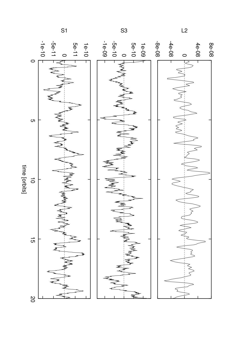
We measure the amplitude and the correlation time of the stochastic forces in all simulations. The results are listed in Table 2. We also plot the time evolution of the azimuthal () force component in Fig. 5. Whereas the correlation time in all simulations is almost the same, the amplitude of the stochastic fluctuations varies by almost a factor of . The forces in the vertical direction are negligible and not presented here. The diffusion coefficient, being a measure of the strength of stochastic forces, is defined as [33, see], where and are the root mean square value and the approximate correlation time of the specific stochastic force in one direction.
| Simulation | Correlation time [s] | Diffusion coefficient [m2 s-3] | Q | |||
|---|---|---|---|---|---|---|
| L2 | cutoff | 5000 | 7000 | 4.1 | ||
| smooth | 6000 | 9000 | ||||
| S1 | cutoff | 2000 | 4000 | 7.2 | ||
| smooth | 3000 | 8000 | ||||
| S3 | cutoff | 2000 | 6000 | 2.5 | ||
| smooth | 4000 | 10000 | ||||
The change in semi major axis due to the effect of stochastic forces with diffusion coefficient after time is given by
| (42) |
where is the mean motion of the moonlet [33]. Note that in this regime, the acceleration of the moonlet doesn’t depend on its mass (as can be seen in Eq. (41)). Therefore, the migration rate and the diffusion coefficient are independent of the mass of the moonlet ; this might be an observational indication for this migration regime.
Assuming an initial semi-major axis of km and m2 s-3 as found in simulation S1, one can calculate the expected difference in semi major axis after one orbit due to stochastic forces which turns out to be m. For simulation S3, assuming m2 s-3, one finds m. For the simulation L2, assuming m2 s-3, one finds m. These translate to random walks with standard deviation given as a function of time by m, m, and m respectively.
IV.3 Discussion
From the above, it can be seen that increasing the surface density by factors changes the migration rate by two orders of magnitude. Thus, the results show clearly that the surface density is much more important than in the regular, type I like migration, presented in Sect. III. This can be easily understood with a toy model. The critical unstable wavelength scales linearly with [42]. If we assume a fixed moonlet size, the ratio of moonlet size to therefore changes with . In the limit where is much smaller than the moonlet radius, the stochastic forces are negligible as the density distribution is approximately homogeneous on the relevant scales. This is the case in simulation S1. In the other limit where is larger than the moonlet, the moonlet undergoes a random walk that is similar to that of individual ring particles, as seen in simulation L2.
The range in migration rates found in simulations shows that over time scales of several years, the migration of a moonlet of mass may be dominated by a random walk in some situations (eg. those in simulations S3 and L2, the latter carried out with particles of radius m). However, in regions of the rings where the surface density is small (eg. simulation S1), the moonlet may be in a regular, non-stochastic migration regime. In that case, the model from Sect. III can be applied.
This dependence offers an exciting possibility to constrain the nature of the ring particles and the physical processes occurring in the rings by measuring the migration of moonlets. But note that because regular migration gives a decrease in the semi-major axis that is linear in time, provided it continues to operate, it will always ultimately dominate the behavior for large time because the spreading of the semi-major axis associated with stochastic migration increases only as the square root of time.
At the present day, the number of observed migration rates is not sufficient to draw a statistically significant conclusion. However, the fact that the migration varies in rate and direction clearly favors the stochastic migration model presented in this section. Considering a migration rate of m in year in Eq. (42), one finds m2 s-3. Taking m in year gives m2 s-3. This is in the range obtained in the simulations, and tends to favor the case of simulation L2, and kg m-2 in the A ring.
V Conclusion
In this paper we have calculated the differential torque exerted on a moonlet by the outer and the inner disk with a smooth, flat surface density profile. We performed both an accurate numerical integration and a second order analytical calculation. These approaches were found to be in excellent agreement where their domains of validity overlap. The migration rate found in this case is proportional to the mass of the moonlet to the power . It is about m yr-1 for a m radius moonlet in the A-ring. This is way too low to explain the observed migration of the propellers in Saturn’s rings. Nonetheless, density fluctuations in the rings, due to their proximity to gravitational instability, can lead to stochastic torques on a moonlet, that may dominate on the timescale of the Cassini mission, to an extent that depends mainly on the surface density of the rings. These stochastic torques may account for the observations.
The possibility that the migration of propellers is induced by stochastic processes rather than by a regular type I like migration is therefore very exciting : this may help to infer the local surface density, and therefore the size of the ring particles. Indeed, both quantities are linked through the optical depth, which is observationally well constrained. Our estimate of kg m-2 is equivalent to m size particles in the A ring for a single-sized population. This is in good agreement with available estimates from stellar occultations. For the A ring, Voyager occultations [46] find that the radius of particles follows : m (assumed) m, with a power index . For the 28 Sgr occultation [15], a range m m is found, with a power index between and , and an effective size (the single average size accounting for the fluctuations in photon count) being about m [12].
Fortunately the Cassini mission has been extended to 2017. In the meantime, numerous observations of the propellers will hopefully give a clear picture of their orbital evolution for a period of 10 years, representing about orbits. This will allow us to test the hypothesis presented in this paper, and in particular to check whether the propellers really are in stochastic migration, whereas first results seem to favor the stochastic hypothesis.
Among the questions that still need to be addressed is why all the propellers seem to be gathered in the A ring, in places apparently devoid of density waves ? Indeed the propellers seem gathered in a couple of narrow radial bands of only about 1000 km width [39]. This is especially surprising since the A ring is densely populated by numerous density waves launched by the nearby small moons (Atlas, Prometheus, Pandora, Janus, Epimetheus). Is there a systematic mechanism that would eject the propellers away from density waves ? Or does the present location of propellers just reflect the initial location of the parent body, assuming that the propeller population comprises the fragments resulting from the destruction of an ancient moon orbiting within the rings ?
If the moonlets really undergo stochastic migration, then Eq. (42) may strongly constrain the age of the propellers, which can’t be larger than the time needed to diffuse over km. Unfortunately, as long as is unknown Eq. (42) doesn’t provide any useful information. However, considering that is proportional to the square root of the time, and assuming that a moonlet migrates about m in year, one finds that km for million years. Assuming m in year, we find that it requires million years to diffuse over km. Note that for m radius moonlets, the spreading due to stochastic migration equates to the contraction of the semi-major axes occurring as a result of smooth, regular migration after yr, and then km. Thus it would take about a million years to migrate through km in this case, largely through the action of the non-stochastic, regular migration process, if that can be assumed to operate smoothly and simultaneously with the stochastic migration process. A m radius moonlet would migrate through only km in the same period, so that the smooth, regular migration process spreads a population of moonlets of various sizes over km in one to two million years. These could be the times since the catastrophic disruption of a small moon orbiting at km from Saturn, that was broken into smaller moonlets by a meteoritic impact. On the other hand, an estimate of the lifetime of a Pan size moon ( km in radius) against the today’s cometary flux is provided by Dones et al. [14] and gives a range between Myr and Gyr, depending on the size distribution of impactors. Therefore, the recent occurrence of such an event, about to billion years after solar system formation, is possible. Note also that an age of about Myr is coherent with some estimates of Saturn’s ring age despite of the lack of fully satisfactory explanation for their origin [see 7, for a review].
We see that the question of propeller’s migration is inextricably linked to the issue of the origin of Saturn’s moons embedded in the rings, which is still a mystery. Porco et al. [29] and Charnoz et al. [6] have jointly proposed that small moons embedded in the rings could be aggregates of material on an initial shard denser than ice. When destroyed by meteoritic bombardment, these could release dense chunks of material that could explain the origin of the propellers. However, the origin of Saturn’s ring system is still a matter of debate [18, 8]. Knowledge of the age of the propellers could provide important constraints on the age of the main ring system and its embedded moons, as there are strong indications that these could have about the same age, provided these moonlets hide a dense shard [6, 29]. Understanding the migration rate of the propellers is therefore an important piece of this puzzle.
Appendix A Evaluation of the Green’s function
Here we evaluate the Green’s function defined by Eq. (15) as
| (A1) |
To perform the summation we use the general result that if for a general periodic function
| (A2) |
with period and being defined as an integrable function, we set
| (A3) |
then
| (A4) |
References
- [1] Balbus, S. A., Hawley, J. F., Jul. 1991. A powerful local shear instability in weakly magnetized disks. I - Linear analysis. II - Nonlinear evolution. ApJ376, 214–233.
- [2] Barnes, J., Hut, P., Dec. 1986. A hierarchical O(N log N) force-calculation algorithm. Nature324.
- [3] Baruteau, C., Masset, F., Jan. 2008. On the Corotation Torque in a Radiatively Inefficient Disk. ApJ672, 1054–1067.
- [4] Bridges, F. G., Hatzes, A., Lin, D. N. C., May 1984. Structure, stability and evolution of Saturn’s rings. Nature309, 333–335.
- [5] Burns, J. A., Tiscareno, M. S., Spitale, J., Porco, C. C., Cooper, N. J., Beurle, K., Jan. 2009. Giant Propellers Outside the Encke Gap in Saturn’s Rings. In: Bulletin of the American Astronomical Society. Vol. 41 of Bulletin of the American Astronomical Society. pp. 559–+.
- [6] Charnoz, S., Brahic, A., Thomas, P. C., Porco, C. C., Dec. 2007. The Equatorial Ridges of Pan and Atlas: Terminal Accretionary Ornaments? Science 318, 1622–.
- [7] Charnoz, S., Dones, L., Esposito, L. W., Estrada, P. R., Hedman, M. M., 2009a. Origin and Evolution of Saturn’s Ring System. In: Dougherty, M. K., Esposito, L. W., Krimigis, S. M. (Eds.), Saturn from Cassini-Huygens. pp. 537–573.
- [8] Charnoz, S., Morbidelli, A., Dones, L., Salmon, J., Feb. 2009b. Did Saturn’s rings form during the Late Heavy Bombardment? Icarus 199, 413–428.
- [9] Colwell, J. E., Esposito, L. W., Sremčević, M., Apr. 2006. Self-gravity wakes in Saturn’s A ring measured by stellar occultations from Cassini. Geophys. Res. Lett.33, 7201–+.
- [10] Crida, A., Charnoz, S., Papaloizou, J., Salmon, J., Sep. 2009. Satellite And Propeller Migration In Saturn’s Rings. Vol. 41 of AAS/DPS Meeting Abstracts. pp. #18.07–+.
- [11] Crida, A., Morbidelli, A., Masset, F., Apr. 2006. On the width and shape of gaps in protoplanetary disks. Icarus 181, 587–604.
- [12] Cuzzi, J., Clark, R., Filacchione, G., French, R., Johnson, R., Marouf, E., L., S., 2009. Ring Particle Composition and Size Distribution. In: Dougherty, M. K., Esposito, L. W., Krimigis, S. M. (Eds.), Saturn from Cassini-Huygens. pp. 459–509.
- [13] Daisaka, H., Tanaka, H., Ida, S., Dec. 2001. Viscosity in a Dense Planetary Ring with Self-Gravitating Particles. Icarus 154, 296–312.
- [14] Dones, L., Chapman, C. R., MacKinnon, B., Kirchoff, M. R., Neukum, G., Zahnle, K. J., 2009. Icy Satellites of Saturn: Impact Cratering and Age Determination. In: Dougherty, M. K., Esposito, L. W., Krimigis, T. (Eds.), Saturn from Cassini-Huygens. pp. 613–635.
- [15] French, R. G., Nicholson, P. D., Jun. 2000. Saturn’s Rings II. Particle sizes inferred from stellar occultation data. Icarus 145, 502–523.
- [16] Goldreich, P., Tremaine, S., Nov. 1979. The excitation of density waves at the Lindblad and corotation resonances by an external potential. ApJ233, 857–871.
- [17] Goldreich, P., Tremaine, S., Oct. 1980. Disk-satellite interactions. ApJ241, 425–441.
- [18] Harris, A. W., 1984. The origin and evolution of planetary rings. In: R. Greenberg & A. Brahic (Ed.), IAU Colloq. 75: Planetary Rings. pp. 641–659.
- [19] Ida, S., Bryden, G., Lin, D. N. C., Tanaka, H., May 2000. Orbital Migration of Neptune and Orbital Distribution of Trans-Neptunian Objects. ApJ534, 428–445.
- [20] Kley, W., Crida, A., Aug. 2008. Migration of protoplanets in radiative discs. A&A487, L9–L12.
- [21] Levison, H. F., Morbidelli, A., Gomes, R., Backman, D., 2007. Planet Migration in Planetesimal Disks. Protostars and Planets V, 669–684.
- [22] Lewis, M. C., Stewart, G. R., Feb. 2009. Features around embedded moonlets in Saturn’s rings: The role of self-gravity and particle size distributions. Icarus 199, 387–412.
- [23] Lin, D. N. C., Papaloizou, J., Mar. 1979. Tidal torques on accretion discs in binary systems with extreme mass ratios. MNRAS186, 799.
- [24] Masset, F. S., Sep. 2001. On the Co-orbital Corotation Torque in a Viscous Disk and Its Impact on Planetary Migration. ApJ558, 453–462.
- [25] Masset, F. S., Papaloizou, J. C. B., May 2003. Runaway Migration and the Formation of Hot Jupiters. ApJ588, 494–508.
- [26] Paardekooper, S., Baruteau, C., Crida, A., Kley, W., Nov. 2009. A torque formula for non-isothermal type I planetary migration - I. Unsaturated horseshoe drag. MNRAS, 1769–+.
- [27] Paardekooper, S., Papaloizou, J. C. B., Apr. 2009. On corotation torques, horseshoe drag and the possibility of sustained stalled or outward protoplanetary migration. MNRAS394, 2283.
- [28] Papaloizou, J. C. B., Nelson, R. P., Kley, W., Masset, F. S., Artymowicz, P., 2007. Disk-Planet Interactions During Planet Formation. In: Protostars and Planets V. pp. 655–668.
- [29] Porco, C. C., Thomas, P. C., Weiss, J. W., Richardson, D. C., Dec. 2007. Saturn’s Small Inner Satellites: Clues to Their Origins. Science 318, 1602–.
- [30] Porco, C. C., West, R. A., Squyres, S. M., Alfred, T. P., Murray, C. D., Del Genio, A., Ingersoll, A. P., Johnson, T. V., Neukum, G., Veverka, J., Dones, L., Brahic, A., Burns, J. A., Haemmerle, V., Knowles, B., Dawson, D., Roatsch, T., Beurle, K., Owen, W., Mar. 2004. Cassini Imaging Science: Instrument Characteristics And Anticipated Scientific Investigations At Saturn. Space Science Reviews 115, 363–497.
- [31] Press, W. H., Teukolsky, S. A., Vetterling, W. T., Flannery, B. P., 1992. Numerical recipes in FORTRAN. The art of scientific computing. Cambridge: University Press, —c1992, 2nd ed.
- [32] Rein, H., Lesur, G., Leinhardt, Z. M., 2010. The Validity of the Super-Particle Approximation during Planetesimal Formation. A&A, in press, ArXiv e–prints 1001.0109.
- [33] Rein, H., Papaloizou, J. C. B., apr 2009. On the evolution of mean motion resonances through stochastic forcing: fast and slow libration modes and the origin of hd 128311. A&A497 (2), 595–609.
- [34] Rein, H., Papaloizou, J. C. B., 2010. Stochatic orbital migration of small bodies in saturn’s rings. A&A, in preparation, available on arXiv.
- [35] Salo, H., Oct. 1995. Simulations of dense planetary rings. III. Self-gravitating identical particles. Icarus 117, 287–312.
- [36] Spahn, F., Sremčević, M., Jun. 2000. Density patterns induced by small moonlets in Saturn’s rings? A&A358, 368–372.
- [37] Sremčević, M., Schmidt, J., Salo, H., Seiß, M., Spahn, F., Albers, N., Oct. 2007. A belt of moonlets in Saturn’s A ring. Nature449, 1019–1021.
- [38] Tanaka, H., Takeuchi, T., Ward, W. R., Feb. 2002. Three-Dimensional Interaction between a Planet and an Isothermal Gaseous Disk. I. Corotation and Lindblad Torques and Planet Migration. ApJ565, 1257–1274.
- [39] Tiscareno, M. S., Burns, J. A., Hedman, M. M., Porco, C. C., Mar. 2008. The Population of Propellers in Saturn’s A Ring. AJ135, 1083–1091.
- [40] Tiscareno, M. S., Burns, J. A., Hedman, M. M., Porco, C. C., Weiss, J. W., Dones, L., Richardson, D. C., Murray, C. D., Mar. 2006. 100-metre-diameter moonlets in Saturn’s A ring from observations of ‘propeller’ structures. Nature440, 648–650.
- [41] Tiscareno et al., 2010. in preparation.
- [42] Toomre, A., May 1964. On the gravitational stability of a disk of stars. ApJ139, 1217–1238.
- [43] Ward, W. R., Jul. 1986. Density waves in the solar nebula - Differential Lindblad torque. Icarus 67, 164–180.
- [44] Ward, W. R., Mar. 1991. Horsehoe Orbit Drag. In: Lunar and Planetary Institute Conference Abstracts. pp. 1463–1464.
- [45] Ward, W. R., Apr. 1997. Protoplanet Migration by Nebula Tides. Icarus 126, 261–281.
- [46] Zebker, H. A., Marouf, E. A., Tyler, G. L., Dec. 1985. Saturn’s rings - Particle size distributions for thin layer model. Icarus 64, 531–548.