Borel generatorsThanks: Version: August 24, 2026
Abstract.
We use the notion of Borel generators to give alternative methods for computing standard invariants, such as associated primes, Hilbert series, and Betti numbers, of Borel ideals. Because there are generally few Borel generators relative to ordinary generators, this enables one to do manual computations much more easily. Moreover, this perspective allows us to find new connections to combinatorics involving Catalan numbers and their generalizations. We conclude with a surprising result relating the Betti numbers of certain principal Borel ideals to the number of pointed pseudo-triangulations of particular planar point sets.
2000 Mathematics Subject Classification
13D02; 13D40; 13F20; 05E401. Introduction
Borel-fixed ideals are arguably the most important ideals in computational commutative algebra. Their combinatorial properties make them easier to investigate than arbitrary monomial ideals, and thanks to work of Galligo [Ga] and Bayer and Stillman [BS87b], we know that generic initial ideals are always Borel-fixed. Moreover, Eliahou and Kervaire show that the minimal graded free resolution of a Borel-fixed ideal in characteristic zero has a particularly nice form [EK]. Thus, as Bayer and Stillman prove in [BS87a], one can determine the regularity of any homogeneous ideal simply by computing the reverse-lex generic initial ideal and determining the highest degree of a minimal generator. Furthermore, lexicographic ideals are Borel-fixed, and thus, by understanding Borel-fixed ideals, we gain valuable insight into the Hilbert functions and graded Betti numbers of arbitrary homogeneous ideals. In addition, papers such as [CE, GHP, Si07] exploit the resolutions of Borel-fixed ideals to obtain minimal free resolutions of closely related monomial ideals as well. Borel-fixed ideals are also of special importance in geometric combinatorics, where they arise in connection with shifted simplicial complexes.
Let , where is a field. We use the term Borel ideal to mean a strongly stable ideal, also known as a 0-Borel-fixed ideal, which is an ideal that is fixed by the Borel group in characteristic zero. Thus the collection of Borel ideals is precisely the collection of generic initial ideals over a field of characteristic zero.
The usual method for studying a Borel ideal is to compute invariants of the ideal in terms of its minimal monomial generating set. In contrast, a few researchers have instead concentrated on the Borel generators of a Borel ideal , a subset of monomials in such that every minimal monomial generator of can be obtained from Borel moves on elements of . For example, Herzog and Srinivasan [HS] prove the Borel case of the Multiplicity Conjectures using Borel generators. Many of the applications of this idea involve principal Borel ideals (ideals with a single Borel generator) in special situations. For example, in [Si08], Sinefakopoulos constructs a shellable polytopal cell complex supporting a minimal free resolution of a principal Borel ideal. Jöllenbeck and Welker also construct a minimal cellular resolution of a principal Borel ideal in [JW]. In addition, Bonanzinga classifies the principal Borel ideals that are lexicographic and investigates which principal Borel ideals are Gotzmann [Bo]. There have also been a number of papers that include results on principal -Borel ideals, including [AH, HPV, JW, Pa, Po].
Our goal in this paper is a bit different. We use the notion of minimal Borel generators of a Borel ideal to develop alternative ways of computing standard invariants in commutative algebra. Our approach has two primary advantages over the traditional ways of doing the computations. First, the number of Borel generators is usually far smaller than the number of ordinary minimal generators of a Borel ideal. Hence when computing invariants of Borel ideals by hand, it is often much easier to use our methods because one does not need to keep track of all the minimal monomial generators of the ideal. This is especially true when working with a principal Borel ideal. Second, our different point of view allows us to uncover connections to combinatorics and computational geometry that are not easily visible using standard techniques. It becomes natural to study principal Borel ideals, which do not appear any more interesting than other Borel ideals from the usual perspective. Using our methods, however, the Catalan numbers and generalizations arise naturally. Investigating principal Borel ideals leads us to an interesting sequence of Betti numbers with a strong connection to pointed pseudo-triangulations. Throughout the paper, we discuss how to apply our techniques to squarefree Borel ideals as well.
Our paper is organized as follows. In Section 2, we explain our terminology and describe how to do some fundamental operations on Borel ideals using only Borel generators. We give two methods for computing the associated primes of a Borel ideal in terms of its Borel generators in Section 3, and we compute the Alexander dual in the squarefree case. In Section 4, we determine a Stanley decomposition for , where is a Borel ideal, which yields a short proof of Stanley’s conjecture in this case. The decomposition also provides formulas for the Hilbert series and multiplicity of . We explain how Catalan numbers and their generalizations arise in the Hilbert functions (and subsequently, the Betti numbers) of Borel ideals in Section 5. In Section 6, we describe how to compute the graded Betti numbers of a Borel ideal using only the Borel generators, and we describe several Poincaré series associated to , where is a Borel or squarefree Borel ideal. Finally, in Section 7, we prove an unexpected connection between the Betti numbers of certain principal Borel ideals and pointed pseudo-triangulations of particular planar point sets studied in [AOSS]. While we often focus on principal Borel ideals, we illustrate how to use our methods for these ideals iteratively to do computations for general Borel ideals.
We gratefully acknowledge the computer algebra system Macaulay 2 [GS], which we used to compute examples throughout this project, and thank Dana Brunson for use of the High Performance Computing Center at Oklahoma State University. The first author was partially supported by an NSA Young Investigator Grant.
2. Preliminaries
Throughout, let , where is a field.
Definition 2.1.
Let be a monomial in . A Borel move on is an operation that sends to a monomial , where for all , and all divide .
Definition 2.2.
A monomial ideal is a Borel ideal if is closed under Borel moves. That is, if , then any monomial obtained from a Borel move on is also in .
When is a Borel ideal, Bayer and Stillman show in [BS87b, Corollary 2] that has an especially nice structure.
Theorem 2.3.
Let be a Borel ideal in . If , then for some .
Notation 2.4.
Given a monomial of degree , we may write uniquely in the form with . We call this expression the factorization of . We say the variable is in the position, and . We will routinely abuse notation and write . We define the minimum similarly, setting (or ).
Example 2.5.
The factorization of is . The variable in the seventh position is , and .
Definition 2.6.
Let be a set of monomials. Define to be the smallest Borel ideal containing . We say that are Borel generators of . If has cardinality one, we say that is the principal Borel ideal generated by .
Remark 2.7.
The computer algebra system Macaulay 2 [GS] has a method for determining the smallest Borel ideal containing a set of monomials . Typing borel monomialIdeal(a*b*e,a*c*d), for example, produces the smallest Borel ideal containing the monomials and .
Definition 2.8.
Factor and . We say that if and for all . In this case, we say that precedes in the Borel order.
Remark 2.9.
If , then . If , then , where is the (ungraded) lexicographic order.
Example 2.10.
and precede , as does , but and are incomparable in the Borel order.
Lemma 2.11.
is spanned as a vector space by the monomials which precede some element of in the Borel order.
Proposition 2.12.
Every Borel ideal has a unique minimal set of Borel generators. We call this set .
Proof.
Given a Borel ideal , let be the minimal monomial generators of . This is a finite set, partially ordered by the Borel order. Let be the minimal monomials in this poset. Clearly . On the other hand, if and is any subset of , then . ∎
In light of Proposition 2.12, we will often refer to as “the Borel generators” of .
Proposition 2.13.
Suppose is a Borel ideal and . Then if and only if for all dividing , both and .
The codimension and projective dimension of a Borel ideal are well-understood, and can be read off from the Borel generators.
Proposition 2.14.
Let be Borel with Borel generators . Then and . If the Borel generators are written in lexicographic order, then .
Proof.
By the Eliahou-Kervaire resolution [EK], the projective dimension of is . Let be a generator of such that is maximal, and be such that precedes in the Borel order. Then .
Let . Then, by Borel moves, contains pure powers of for all ; thus . On the other hand, every monomial of is contained in , so . ∎
All basic operations on Borel ideals can be performed in terms of only their Borel generators.
Proposition 2.15.
Let and for sets of monomials and . Then .
Proposition 2.16.
Let and be written in factored form, and suppose that . Put (with if ), and let be the meet of and in the Borel order. Then .
Using the two propositions above, many computations on a Borel ideal can be done in terms of principal Borel ideals. One first works with for each , then combines the results (possibly using inclusion-exclusion). Such an approach allows simpler notation, so we will adopt it without comment wherever possible in the remainder of the paper.
Proposition 2.17.
Corollary 2.18.
Let be the homogeneous maximal ideal. Then we have .
Proposition 2.19.
Write in factored form, and let be minimal such that . Then . If instead , then the colon ideal is .
2.1. Squarefree Borel ideals
Definition 2.20.
We say that an ideal is squarefree if it is generated by squarefree monomials and squarefree Borel if it is generated by the squarefree monomials of some Borel ideal. For a set of squarefree monomials , the squarefree Borel ideal generated by is the smallest squarefree Borel ideal containing , denoted .
Almost all the results on Borel ideals stated above hold (with appropriate modification) for squarefree Borel ideals. For example, is generated by the squarefree monomials which precede some monomial of in the Borel order. The exceptions are Proposition 2.17, which doesn’t make sense in the squarefree context, and Proposition 2.14 and Corollary 2.18 which become:
Proposition 2.21.
Let be squarefree Borel with Borel generators . The projective dimension of is . The codimension of is .
Proof.
Proposition 2.22.
Let be the homogeneous maximal ideal, and let be maximal such that does not divide . Then the squarefree part of is .
3. Associated primes
In this section, we compute the associated primes of a Borel ideal. Our main tools are the following:
Theorem 3.1 (Bayer-Stillman).
Suppose that is an associated prime of the Borel ideal . Then for some .
Theorem 3.2.
Suppose that is an associated prime of the Borel ideal . Then there exists some Borel generator such that and .
Throughout the section, is a Borel ideal.
Notation 3.3.
If is a squarefree monomial, write for the prime ideal on the support of , . If , write for the prime ideal .
Definition 3.4.
is a -socle for if .
Lemma 3.5.
Suppose is a -socle for . Assume that for all dividing , and are not -socles. Then .
Proof.
Because , . Thus, we must show that and for any dividing .
First, we show that . Suppose it were in . Then by the Borel move taking to . If , it would follow that , contradicting the fact that is a -socle. Hence . Therefore , meaning . Because is Borel, this implies that . Since is not a -socle, there is a monomial in the variables in , and hence for some . Multiplying by proves that , contradicting the fact that is a -socle.
We now prove that . Suppose it were, and let . Then , and thus . By hypothesis, is not a -socle, so for some . After a Borel move sending to , we have , contradicting the fact that is a -socle. Therefore . ∎
Proof of Theorem 3.2.
If , then there is some monomial which is a -socle. If there is a variable and a monomial of the form or which is also a -socle, replace with . This process must terminate since there are finitely many monomials of degree at most . Thus, without loss of generality, the -socle may be chosen to satisfy the hypotheses of Lemma 3.5. Hence we may take . ∎
Theorem 3.2 yields the following efficient algorithm for computing when is a Borel ideal.
Algorithm 3.6.
This algorithm computes for a Borel ideal .
-
For each , do the following:
- Step 1:
List all the which are divisible by .
- Step 2:
For each identified in Step 1, determine if is a -socle. If it is, then is associated to . If none are, then is not associated.
If is a principal Borel ideal, it is possible to read off without having to verify any annihilators, as the next proposition shows.
Proposition 3.7.
Suppose that and divides . Then is a -socle.
Proof.
Clearly . Thus, if were not a -socle, we would have for large . But does not precede in the Borel order for any positive . ∎
Corollary 3.8.
Suppose that is a principal Borel ideal. Then if and only if divides .
We thank the referee for suggesting the following corollary.
Corollary 3.9.
Let be any set of prime ideals all having the form . Then there exists a principal Borel ideal such that . Moreover, if and only if .
We would like to be able to determine for a general Borel ideal while avoiding socle computations entirely. The notion of -truncation, defined below, will allow us to do this.
Definition 3.10.
Let be a monomial with factorization , and let be a positive integer. If , define the -truncation of , denoted , to be . If , then set to be itself. For a monomial ideal , define the -truncation of to be the ideal .
Example 3.11.
The -truncation of is , while the -truncation of is itself for .
Lemma 3.12.
Let be a Borel ideal. Then
In particular, the -truncation of a Borel ideal is Borel.
Remark 3.13.
It is not the case that for an arbitrary monomial ideal . For example, let and put . Then the right-hand side above is . However, , so the left-hand side contains .
Proof of Lemma 3.12.
It suffices to show . Suppose that . Then there is some such that . Thus, there is some Borel generator for such that precedes in the Borel order. It follows that precedes in the Borel order, so as desired. ∎
We begin with some observations about how -socles relate to the -truncations of Borel generators.
Lemma 3.14.
Let be a Borel ideal, and suppose . Let be the maximal index such that is in the position in . Set . Then is a -socle for if and only if is a -socle for .
Proof.
Write .
First, suppose that is a -socle for . If were not a -socle for , it would follow that for some large . Since is generated in degrees less than or equal to , it follows that . Thus there is a Borel generator of which is preceded in the Borel order by , and a Borel generator of such that . Observe that, for some , has in the place; in particular . We may multiply by any monomial without leaving , so in particular, it follows that for greater than the degree of .
Thus we have
Applying Borel moves, we have
for nonnegative integers and . Rearranging,
contradicting the assumption that is a -socle for .
Conversely, suppose that is not a -socle for . Then, since , it follows that for some . In particular, , so that is not a -socle for .
∎
Lemma 3.15.
Let be a Borel ideal, and suppose is a monomial with . If and for all , then is a -socle.
Proof.
Note that , meaning . If is not a -socle, then for some large . Consequently, is divisible by some monomial in of degree , which must be . Hence , but this contradicts . Therefore is a -socle. ∎
Algorithm 3.16.
This algorithm computes for a Borel ideal without computing socles. Suppose is generated in degree at most .
- Step 1:
For , compute .
- Step 2:
For each of degree , .
- Step 3:
List all primes found in Step 2.
The trade-off with Algorithm 3.6 is clear. In Algorithm 3.6, for each Borel generator, one has to compute the annihilator of several monomials (or at least compute enough to know whether it is possible for to be a -socle). In Algorithm 3.16, one needs to compute the Borel generators of all of the -truncations of , but can then read off directly from that list of Borel generators with no further work.
We prove that Algorithm 3.16 gives a complete list of the primes in .
Proof of Algorithm 3.16.
We begin by proving that the algorithm identifies all elements of . We induct on , the maximum degree of a minimal generator of . Let , and suppose . If , then , and the algorithm identifies .
If , then there exists such that is a -socle. Let be the maximum position of in . If , then the algorithm identifies from . If not, then by Lemma 3.14, is a -socle for . Therefore is associated to . Because , by induction, the algorithm identifies .
Conversely, we need to prove that any prime that Algorithm 3.16 returns is actually in . Suppose there exists a positive integer such that is a monomial of degree in , and . Then by Lemma 3.15, is a -socle for . Let be the monomial last in lex order among those monomials whose -truncation is . We have two cases to consider.
First, suppose does not have in position . Then by Lemma 3.14, is a -socle for . Therefore . If does have in position , let be maximal such that has in position . Now is a minimal Borel generator of by the choice of , and, by Lemma 3.15, is a -socle for , and does not have in the position. Thus, Lemma 3.14 applies, and as above. ∎
Example 3.17.
Consider the ideal in . Then , which shows that is an associated prime. Moreover, , giving the new prime . The 2-truncation is , so we have another associated prime, . Finally, , giving no new associated primes because is not a Borel generator of the 1-truncation. Therefore .
3.1. Associated primes for squarefree Borels (Alexander duals)
The associated primes of a squarefree ideal correspond to the generators of its Alexander dual, so if is squarefree Borel, computing is equivalent to computing . Because (since ), it suffices to compute for principal squarefree Borel ideals .
Theorem 3.18.
Let be a squarefree monomial, and . Then
Proof.
Note that if and only if for all , is divisible by at least variables with index at most . Let .
Suppose that and is a monomial in . We will show that . Observe that for some , precedes the monomial in the Borel order. If on the contrary , then would be divisible by none of the variables of , so the variables which divide and have indices less than or equal to must all be among the variables in the set , which has cardinality at most .
Conversely, suppose that a monomial is contained in for all squarefree . We will show that . If , then there is some for which is divisible by at most variables with indices less than or equal to . Denote these variables by with . Put . Then we have , but , a contradiction. ∎
Remark 3.19.
Observe that if , then , so the former generator is redundant. Thus, in applying Theorem 3.18, we need only write down the monomials for indices such that .
4. Stanley decompositions
In this section, we describe a Stanley decomposition for , where is any Borel ideal. Recall that, for a multigraded -module , a Stanley decomposition of is a direct sum decomposition
where is some subset of the multigraded elements of (in the case of a quotient of by a monomial ideal, these are monomials) and is a subset of the variables. See, for example, [PFTY] for background and connections to the notion of Stanley depth, the subject of much work in combinatorial commutative algebra. Herzog, Vladoiu, and Zheng investigate Stanley decompositions of Borel ideals in considerably greater generality in [HVZ] than we do here. The primary focus of [HVZ] is computing the Stanley depth of arbitrary monomial modules, i.e., identifying decompositions in which none of the are small. We take a more constructive approach and are interested only in creating an explicit description of one Stanley decomposition of , which we will use to study Hilbert functions. As a bonus, our Stanley decomposition turns out to realize the Stanley depth.
Given a Borel ideal , observe that the truncations of form a filtration of ,
where is the maximal degree of a generator of . Taking quotients yields a filtration of ,
Every monomial of occurs in a smallest term in this filtration; we will use this fact to build a Stanley decomposition.
Theorem 4.1.
Let be a Borel ideal, generated in degrees less than or equal to . Then has the Stanley decomposition
Proof.
First, we will show that each of the summands above has trivial intersection with . Let be given with , and write for the set of variables . Suppose that is a monomial. Since , it follows that . Hence, and has degree . We claim that . It suffices to show that every variable of has greater index than . Suppose to the contrary that has earlier index. Then, in particular, . On the other hand, there exists some monomial with . Thus, for some monomial with . Let . Then , and , a contradiction.
Next, we will show that the summands have pairwise trivial intersection. Let and be two such summands, and suppose that is a monomial in their intersection. Let and be the degrees of and , respectively. Observe that and . Since , it follows that . Without loss of generality, we may assume . Thus, divides , so, in particular, . Let . On the one hand, since , we have . On the other hand, since , we have .
Finally, we will show that every monomial of occurs in one of the summands above. Let be such a monomial. Clearly, . Thus, there is some maximal such that . Let . Then has degree and is a generator of , and . ∎
Recall that the Stanley depth of a module is the maximum, over all Stanley decompositions, of the smallest size of any appearing in the decomposition.
Theorem 4.2.
The Stanley decomposition in Theorem 4.1 realizes the Stanley depth of .
Proof.
Let be maximal such that divides some Borel generator of . Observe that the smallest appearing in the decomposition of Theorem 4.1 is , realized when for any divisible by . (This is minimal because every in this decomposition is a terminal sequence of variables.) Fix one such .
Now let be another Stanley decomposition of . Then appears in some summand in . Thus, for all , . In particular, . Thus, maximizes the minimum dimension of a summand over all Stanley decompositions. ∎
Stanley [St82] conjectured that the Stanley depth of a multigraded module is greater than or equal to its depth. This conjecture is proved for a large class of monomial modules, which includes Borel ideals and quotients by Borel ideals, by Herzog, Vladoiu, and Zheng [HVZ]. The decomposition above yields a much more direct proof for quotients by Borel ideals, and furthermore shows that equality holds in this case.
Corollary 4.3.
Stanley’s conjecture is sharp for quotients by Borel ideals.
Proof.
We can rewrite the summation of Theorem 4.1 in terms of certain quotient modules, without any use of truncation, as follows:
Theorem 4.4.
Let be Borel. Then has the Stanley decomposition
where is the standard monomials of . The index set is empty unless .
Proof.
We have a filtration
Observe that is a summand in the Stanley decomposition of Theorem 4.1 if and only if and , if and only if is a nonzero monomial of and . Every standard monomial modulo has max at most , so the summands of the form are in one-to-one correspondence with the standard monomials of the Artinian module . ∎
Since each summand of the form contributes a summand of to the Hilbert series, Theorem 4.4 yields the following formula for the Hilbert series of :
This formula lacks aesthetic appeal, but it allows us to compute the multiplicity of .
Proposition 4.5.
Write , and let . Then the multiplicity of is
Proof.
The first nonzero summand is because when . All other summands have lower powers of in the denominator. Evaluating the -polynomial at thus gives us . ∎
In the case that is a principal Borel ideal, Theorem 4.1 yields a more elegant expression for the Hilbert series of . Factor . Then, if is a monomial generator of , we compute . Thus, in particular, . This proves the following:
Proposition 4.6.
Let be a principal Borel ideal, and factor . Then
where is the number of degree generators of . The multiplicity of is .
In the next section, we will compute the using generalized Catalan triangles.
5. Catalan diagrams
We begin by recalling some useful notation in the study of Hilbert functions and Betti numbers of Borel ideals.
Definition 5.1.
Let be a Borel (or squarefree Borel) ideal. Write in terms of its minimal monomial generators. For each , , and each degree let be the cardinality of the set and put
If is a (principal) Borel ideal generated in degree , we simply write instead of .
The numbers were introduced by Bigatti in [Bi] and have been used to study Hilbert functions and Betti numbers of Borel ideals, particularly in comparison to lex ideals. See [Bi, Fr, Gr, MP].
In the formula in Proposition 4.6, the number is .
The remainder of this section deals with the computation of for a principal Borel ideal .
Definition 5.2.
For a monomial with factorization , define the Catalan diagram with shape , written , as follows. First construct a left-justified array of boxes whose row (from the top) has boxes. Then put a in each box along the top row. Finally, fill in the remaining boxes by the following rule: the entry in the box of the row is the sum of the entries in the first boxes of the row. (If the row has fewer than boxes, simply fill in the box with the sum of all the entries in the row.) Note that we number rows from top to bottom and columns from left to right, starting with 1 in both cases.

Example 5.3.
If , we can read off the numbers from , the Catalan diagram with shape .
Theorem 5.4.
The entry in the box of the bottom row of is .
Proof.
Let . We induct on . If , then , so and for . Now suppose , , and consider the map from to defined by . This map is clearly injective. By induction, the cardinality of the latter set is the sum of the entries in the first boxes of the row of . To see that this map is surjective, let be a monomial of with degree . Then , so because . So , and the claim follows. ∎
Implicit in this construction is a bijection between generators of a principal Borel ideal and planar lattice paths within the diagram . This is a special case of a lattice path polymatroid; see [Sc].
Example 5.5.
Consider . Then the Catalan diagram with shape is a rectangle with height and width . This is Pascal’s triangle, with the row of Pascal’s triangle along the antidiagonal. The entry in the box of the row is . In particular, .
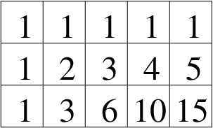
Example 5.6.
Let . We compute the Hilbert series of the quotient . The Catalan diagram is computed in Figure 1. For , the number of generators of is the sum of the entries in the row of this diagram. (Recall that has a single generator.) Thus we compute , and (the first five Catalan numbers). By Corollary 4.6, the Hilbert series of is
has multiplicity one (the coefficient on ) and -polynomial . Since the resolution is linear, we can read off the Betti numbers from .
Example 5.7.
Suppose that is a lexicographic ideal. Then, by [Bo, Prop. 3.2(i)], has the form . A straightforward lattice-path argument on shows that . Some manipulation yields . In particular, the Macaulay representation of , which governs the growth of the Hilbert function of , has the property that the numerators decrease by exactly one between consecutive summands.
Next, we relate Catalan diagrams to squarefree Borel ideals.
Let be a squarefree monomial, with . Define a (not necessarily squarefree) monomial by
Note that is the inverse to the map defined in [AHH00].
Proposition 5.8 ([AHH00]).
The map is a bijection between the squarefree monomials and the monomials of .
Corollary 5.9.
If is a squarefree monomial, is a bijection between and .
Corollary 5.10.
Let be a squarefree monomial of degree , and put and . Then for all .
Proof.
For any monomial of degree , if and only if . ∎
Now let for some squarefree monomial . By Corollary 5.10, we can compute the numbers : is the entry in the bottom row of .
6. Betti numbers
It is well known that the Betti numbers of a Borel ideal depend only on the . (See, for example, [Bi].) We recall the Eliahou-Kervaire resolution [EK], which makes the necessary computation explicit.
Construction 6.1.
Let be a Borel ideal, and let be a minimal monomial generator of with . Let be any squarefree monomial in . The formal symbol is called an Eliahou-Kervaire symbol or EK symbol for . We assign the EK symbol homological degree equal to the degree of and multidegree equal to .
Theorem 6.2 ([EK]).
The Eliahou-Kervaire symbols form a basis for a minimal free resolution of the ideal .
A nice exposition of the Eliahou-Kervaire resolution in terms of mapping cones is [PS]. This is one of the only known explicit resolutions, so it has been heavily studied; see, for example, [BW, CE, Cl, GHP, Me].
Corollary 6.3.
The graded Betti number is the number of Eliahou-Kervaire symbols with homological degree and internal degree . The graded Betti number is 1 if and otherwise.
For a given monomial generator , the number of such that is an EK symbol of homological degree is . Summing over all gives us a formula for the Betti numbers in terms of the :
Proposition 6.4.
Suppose that is generated entirely in degree . Then
The graded Poincaré series for is
Example 6.5.
Suppose is the power of the maximal ideal. Then , and . This has been known since before the Eliahou-Kervaire resolution was discovered; see for example [BR].
Corollary 6.6.
Suppose that is a principal Borel ideal. Let be the Catalan diagram of shape , and let be the generating function with coefficients given by the bottom row of . Then is the generating function for , and the Poincaré series for is .
Proposition 6.4 enables us to compute the Betti numbers for an arbitrary Borel ideal, one Borel generator at a time:
Lemma 6.7.
Suppose that , with for all . Put and . Then is generated entirely in degree and .
Example 6.8.
We compute the Betti numbers of , a special case of [EK, Example 2], in which Eliahou and Kervaire point out that Catalan numbers arise in computing total Betti numbers of . By Proposition 2.16, . Applying Lemma 6.7, we have
The only row in the Catalan diagram of shape is (1), the bottom row of the Catalan diagram of shape is , and for , it is . Multiplying by the appropriate binomial coefficients, we calculate that , , and of are one, and the other graded Betti numbers are zero.
Let , , and . To get the graded Betti numbers of , we compute and use Lemma 6.7. The bottom row of the Catalan diagram of shape is ; for , the bottom row is , and for , the bottom row is . To compute the graded Betti numbers of , note that the bottom row of the Catalan diagram of shape is . Thus, after multiplying by the binomial coefficients, we have the following graded Betti diagrams, switching to the quotients to use the standard Macaulay 2 output:
| : | total: | 1 | 2 | 1 | : | total: | 1 | 10 | 15 | 6 | : | total: | 1 | 8 | 11 | 4 | ||
| 0: | 1 | 1 | . | 0: | 1 | . | . | . | 0: | 1 | . | . | . | |||||
| 1: | . | 1 | 1 | 1: | . | . | . | . | 1: | . | . | . | . | |||||
| 2: | . | 10 | 15 | 6 | 2: | . | 8 | 11 | 4 |
Adding the first two diagrams and subtracting the third, we obtain the graded Betti diagram of :
| : | total: | 1 | 4 | 5 | 2 |
|---|---|---|---|---|---|
| 0: | 1 | 1 | . | . | |
| 1: | . | 1 | 1 | . | |
| 2: | . | 2 | 4 | 2 |
In a different direction, our techniques also allow us to consider the resolution of the residue field over , where is a Borel ideal. We may assume that is generated by monomials of degree at least two. Then by [Pe, Corollary 1.2], is Golod, and hence the graded Poincaré series of over can be expressed as
Proposition 6.9.
Let be a Borel ideal generated in a single degree , and let be the generating function on the . Then
If is principal, let be the generating function on the bottom row of . Then
Proof.
Because counts the number of elements of with , we have
6.1. Betti numbers for squarefree Borel ideals
Now suppose that is a squarefree Borel ideal in . Then is resolved by the squarefree part of the Eliahou-Kervaire resolution [CE, AHH98]; that is, the basis for the resolution is given by EK symbols with squarefree multidegree. Thus the Poincaré series of is given by
For the rest of the section, assume that is a squarefree Borel ideal generated in a single degree , and let be the generating function on the . If is principal squarefree Borel, let be the generating function on the last row of the Catalan diagram . Recall that .
Proposition 6.10.
The graded Poincaré series of over is
If is principal squarefree Borel, then
Proof.
We have
By [AHH98], the ring is Golod. Thus an argument analogous to that of Proposition 6.9 gives the following formula for the resolution of over :
Proposition 6.11.
The Poincaré series for over is
If is principal squarefree Borel, the graded Poincaré series is
Aramova, Herzog, and Hibi [AHH97] compute the minimal free resolution of a squarefree Borel ideal in the exterior algebra . In [AHH97, Corollary 3.3], they give the graded Poincaré series:
Let . Then a squarefree Borel ideal is naturally defined over in the same way that it is over . The same mapping cone argument minimally resolves over both and , so the Poincaré series is the same in both cases. When is generated in a single degree, this simplifies using the :
Proposition 6.12.
The graded Poincaré series of over or is
If is principal squarefree Borel, then
7. Pointed pseudo-triangulations
In this section, we uncover a surprising connection between the Betti numbers of some principal Borel ideals and the number of pointed pseudo-triangulations of certain point sets in the plane. Fix a monomial with , and consider the principal Borel ideal . We begin by determining a simple expression, not requiring a sum, for the Betti numbers of particular principal Borel ideals. Since principal Borel ideals have linear resolutions, we suppress the degree and write total Betti numbers throughout.
Proposition 7.1.
For each , we have
Proof.
Consider the set of pairs
where each is a squarefree monomial, and note that . We mention that pairs in are not necessarily EK symbols, as we allow to occur in .
Now write as the disjoint union , where and .
When , if and only if . Therefore, the map
gives a bijection between and EK symbols of such that . Thus .
Now let be an EK symbol of with , and consider the map
We claim this map gives a bijection between such EK symbols and pairs in . Clearly, is a generator of counted by . Now let , let , and let . Since , , is a generator of , meaning the map
is an inverse to the above map. Therefore, , and the result follows. ∎
Example 7.2.
When , a power of the maximal ideal, the recursion gives
Recall from Example 5.3 that , the Catalan number. Thus this ideal is interesting from a combinatorial perspective. The following is a special case of Proposition 7.1.
Corollary 7.3.
For any , the following recursion holds:
Proposition 7.4.
For all and all ,
Remark 7.5.
This is an alternate formula for the unsigned version of sequence A062991 in the Online Encyclopedia of Integer Sequences [Sl] (with the indexing shifted). It is listed in a comment in the entry in the OEIS, but no proof is given, so we sketch the argument below.
Proof.
We outline the computational proof, inducting on . When , the Betti number is one, and all other Betti numbers are zero, consistent with the formula. Assume now that the formula is true for some integer , where , for all values of . By Corollary 7.3,
Using the inductive hypothesis, we have
The intermediate computations simply involve factoring out and the appropriate binomial coefficients; then one checks that what remains is equal to one. ∎
The (unsigned version of) sequence A062991 in [Sl] that gives Betti numbers of the ideals also arises in the paper [AOSS], which is devoted to counting pseudo-triangulations of particular point sets. For full details on the combinatorial terminology, see [AOSS]. Briefly, a pseudo-triangle is a polygon in the plane with exactly three convex vertices with internal angles measuring less than . A pseudo-triangulation is a partition of the convex hull of a point set in the plane into pseudo-triangles whose vertex set is exactly . We say that a pseudo-triangulation is pointed if every vertex has an incident angle greater than . Pointed pseudo-triangulations have arisen in a number of settings recently; see, for example, [RSS]. A set of points in the plane a single chain if consists of points labeled that form a convex -gon and one additional point labeled , outside the -gon, but from which all edges but are visible. Let be the number of pointed pseudo-triangulations of in which the point is connected to exactly of the points . (By [AOSS, Theorem 6], these numbers also count certain triangulations of particular convex -polygons.)
Theorem 7.6.
Let be as above. Then .
Proof.
It is enough to show that the Betti numbers satisfy the same recursion as the after the shifting of indices. The recursion for the is [AOSS, Theorem 14], which states that
for , , and . Translating the last two conditions, we need to show that and . Both of these formulas follow from the Eliahou-Kervaire resolution and the counts in the previous section. Rewriting the recursive formula for the in the new indexing, we also need to prove that
This follows from Corollary 7.3 (rewriting as ). ∎
In light of the surprising connection in Theorem 7.6, we close with two questions:
Question 7.7.
Question 7.8.
Suppose we change the set to a different point configuration. Do the analogous correspond to the Betti numbers of other (in special cases, possibly principal) Borel ideals?
References
- [AOSS] O. Aichholzer, D. Orden, F. Santos, and B. Speckmann, On the number of pseudo-triangulations of certain point sets. J. Combin. Theory Ser. A 115 (2008), no. 2, 254–278.
- [AH] A. Aramova and J. Herzog, -Borel principal ideals. Illinois J. Math. 41 (1997), no. 1, 103–121.
- [AHH97] A. Aramova, J. Herzog, and T. Hibi, Gotzmann theorems for exterior algebras and combinatorics. J. Algebra 191 (1997), no. 1, 174–211.
- [AHH00] A. Aramova, J. Herzog, and T. Hibi, Shifting operations and graded Betti numbers. J. Algebraic Combin. 12 (2000), no. 3, 207–222.
- [AHH98] A. Aramova, J. Herzog, and T. Hibi, Squarefree lexsegment ideals. Math. Z. 228 (1998), no. 2, 353–378.
- [BW] E. Batzies, V. Welker, Discrete Morse theory for cellular resolutions. J. Reine Angew. Math. 543 (2002), 147–168.
- [BS87a] D. Bayer and M. Stillman, A criterion for detecting -regularity. Invent. Math. 87 (1987), no. 1, 1–11.
- [BS87b] D. Bayer and M. Stillman, A theorem on refining division orders by the reverse lexicographic order. Duke Math. J. 55 (1987), no. 2, 321–328.
- [Bi] A. M. Bigatti, Upper bounds for the Betti numbers of a given Hilbert function. Comm. Algebra 21 (1993), no. 7, 2317–2334.
- [Bo] V. Bonanzinga, Principal Borel ideals and Gotzmann ideals. Arch. Math. 81 (2003), 385–396.
- [BR] D. Buchsbaum and D. S. Rim, A generalized Koszul complex. II. Depth and multiplicity, Trans. Amer. Math. Soc. 111 (1964), 197–224.
- [CE] H. Charalambous and E. G. Evans, Jr., Resolutions obtained by iterated mapping cones. J. Algebra 176 (1995), no. 3, 750–754.
- [Cl] T. B. P. Clark, A minimal poset resolution of stable ideals, preprint, 2008. arXiv:0812.0594
- [EK] S. Eliahou and M. Kervaire, Minimal resolutions of some monomial ideals. J. Algebra 129 (1990), no. 1, 1–25.
- [Fr] C. A. Francisco, Minimal graded Betti numbers and stable ideals. Comm. Algebra 31 (2003), no. 10, 4971–4987.
- [Ga] A. Galligo, À propos du théorème de-préparation de Weierstrass. Fonctions de plusieurs variables complexes. Lect. Notes Math. 409 (1974), 543–579.
- [GHP] V. Gasharov, T. Hibi, and I. Peeva, Resolutions of -stable ideals. J. Algebra 254 (2002), no. 2, 375–394.
- [GS]
D. R. Grayson and M. E. Stillman, Macaulay 2, a software system for research in algebraic geometry.
http://www.math.uiuc.edu/Macaulay2/. - [Gr] M. Green, Generic initial ideals. Six lectures on commutative algebra (Bellaterra, 1996), 119–186, Progr. Math. 166, Birkhäuser, Basel, 1998.
- [HPV] J. Herzog, D. Popescu, and M. Vladoiu, On the Ext-modules of ideals of Borel type. Commutative algebra (Grenoble/Lyon, 2001), 171–186, Contemp. Math. 331, Amer. Math. Soc., Providence, RI, 2003.
- [HS] J. Herzog and H. Srinivasan, Bounds for multiplicities. Trans. Amer. Math. Soc. 350 (1998), no. 7, 2879–2902.
- [HVZ] J. Herzog, M. Vladoiu, and X. Zheng, How to compute the Stanley depth of a monomial ideal. J. Algebra 322 (2009), no. 9, 3151–3169.
- [JW] M Jöllenbeck and V. Welker, Minimal resolutions via algebraic discrete Morse theory. Mem. Amer. Math. Soc. 197 (2009), no. 923, vi+74 pp.
- [Ko] T. Koshy, Catalan Numbers with Applications, Oxford University Press, New York, 2008.
- [Me] J. Mermin, The Eliahou-Kervaire resolution is cellular. J. Commut. Algebra 2 (2010), no. 1, 55–78.
- [MP] J. Mermin and I. Peeva, Hilbert functions and lex ideals. J. Algebra 313 (2007), no. 2, 642–656.
- [NR] U. Nagel and V. Reiner, Betti numbers of monomial ideals and shifted skew shapes. Electron. J. Combin. 16 (2009), no. 2, Special volume in honor of Anders Bjorner, Research Paper 3, 59 pp.
- [Pa] K. Pardue, Nonstandard Borel-fixed ideals, Dissertation, Brandeis University, 1994.
- [Pe] I. Peeva, 0-Borel fixed ideals. J. Algebra 184 (1996), no. 3, 945–984.
- [PS] I. Peeva and M. Stillman, The minimal free resolution of a Borel ideal. Expo. Math. 26 (2008), no. 3, 237–247.
- [Po] D. Popescu, Binomial cycle bases on Koszul homology modules. Comm. Algebra 36 (2008), no. 5, 1789–1800.
- [PFTY] M. Pournaki, S. A. Seyed Fakhari, M. Tousi, and S. Yassemi, What is Stanley depth? Notices Amer. Math. Soc. 56 (2009), no. 9, 1106–1108.
- [RSS] G. Rote, F. Santos, and I. Streinu, Expansive motions and the polytope of pointed pseudo-triangulations. Discrete and computational geometry, 699–736, Algorithms Combin. 25, Springer, Berlin, 2003.
- [Sc] J. Schweig, On the -vector of a lattice path matroid. Electron. J. Combin. 17 (2010), no. 1, Note 3, 6 pp.
- [Si08] A. Sinefakopoulos, On Borel fixed ideals generated in one degree. J. Algebra 319 (2008), no. 7, 2739–2760.
- [Si07] A. Sinefakopoulos, On special -Borel ideals, preprint, 2007. arXiv:0702628v1
- [Sl] N. J. A. Sloane, (2009), The On-Line Encyclopedia of Integer Sequences, published electronically at http://www.research.att.com/njas/sequences/.
- [St99] R. P. Stanley, Enumerative Combinatorics, Volume 2, Cambridge University Press, Cambridge, UK, 1999.
- [St82] R. P. Stanley, Linear Diophantine equations and local cohomology. Invent. Math. 68 (1982), no. 2, 175–193.