跳到论文正文
W Papers独立论文阅读器 arXiv:1006.1340 论文正文 计算阅读时间 · 0%
引用这篇论文根据当前论文元数据生成,正式投稿前建议核对。


License: arXiv.org perpetual non-exclusive license
arXiv:1006.1340v1 [math.CO] 07 Jun 2010

Control of cancellations that restrain the growth of a binomial recursionThanks: The second author was supported by NSF grant DMS-0701557

Magnus Aspenberg and Rodrigo Pérez Address: LD-224R IUPUI, 402 N. Blackford St., Indianapolis, IN 46202, USA Email address: rperez@math.iupui.edu
Abstract.

We study a recursion that generates real sequences depending on a parameter xx. Given a negative xx the growth of the sequence is very difficult to estimate due to canceling terms. We reduce the study of the recursion to a problem about a family of integral operators, and prove that for every parameter value except −1-1, the growth of the sequence is factorial. In the combinatorial part of the proof we show that when x=−1x=-1 the resulting recurrence yields the sequence of alternating Catalan numbers, and thus has exponential growth. We expect our methods to be useful in a variety of similar situations.

1. Introduction

Fix an arbitrary real number x≠0x\neq 0, and consider the sequence defined by the recursive expression

(1) a1=x,an=x​∑r=⌈n2⌉n−1(rn−r)​ar.a_{1}=x\quad,\qquad a_{n}=x\sum_{r=\left\lceil\frac{n}{2}\right\rceil}^{n-1}{\displaystyle\binom{r}{n-r}}a_{r}.

For x=1x=1, formula (1) produces the sequence 1,2,7,34,214,1652,…1,2,7,34,214,1652,\ldots Note that the last summand (n−11)​an−1{\textstyle\binom{n-1}{1}}a_{n-1} guarantees that an>(n−1)!a_{n}>(n-1)! This means that {an}\{a_{n}\} grows very fast since n!>(n/e)n\displaystyle n!>(n/e)^{n}. We prove

Theorem 1.

For any real x≠−1,0x\neq-1,0 the sequence {an}\{a_{n}\} defined by (1) grows super-exponentially.

This is an interesting behavior, and not altogether obvious because when x<0x<0, there are a lot of cancellations. In fact, when x=−1x=-1, the positive and negative terms exactly balance out to yield a surprising contrast:

Theorem 2.

When x=−1x=-1, formula (1) produces the sequence (−1)n​Cn(-1)^{n}C_{n} of Catalan numbers with alternating signs, and therefore grows exponentially.

The phenomenon at play is very interesting. In the first part of the paper some combinatorial constructions will allow us to prove the results when x>0x>0 and when x≤−1x\leq-1. However, when x∈(−1,0)x\in(-1,0), the cancellations and the small size of xx conspire to render elementary arguments ineffective. In the second part we introduce functional analytic methods to control the effect of the cancellations in that case. We expect these ideas to be useful in a variety of similar situations.

1.1. Structure

The paper has two parts. In the first (sections 2 to 4) we prove Theorem 2 and the case x∉[−1,0]x\notin[-1,0] of Theorem 1. Section 2 presents some basic facts about hypercube graphs and the Catalan numbers; Section 3 defines the combinatorial structure we use; and Section 4 contains the proofs.

The second part (sections 5 to 7) tackles the case x∈(−1,0)x\in(-1,0) of Theorem 1. Section 5 uses the combinatorial knowledge gained in the first part to derive an alternative expression for ana_{n} as the sum of a sequence of numbers Sn​(1),…,Sn​(n−1)S_{n}(1),\ldots,S_{n}(n-1) constructed recursively. This sequence is translated into a function sn∈L2​[0,1]s_{n}\in L^{2}[0,1], and the recursion is interpreted as an integral operator. Section 6 contains the proof of the theorem assuming the statement of Lemma 10, and Section 7 is devoted to the proof of Lemma 10.

2. Basic Combinatorial Facts

2.1. Hypercubes

The hypercube graph ℋn\mathcal{H}_{n} is the graph whose set of vertices VnV_{n} consists of all nn-vectors with coordinates 𝟢{\sf 0} or 𝟣{\sf 1}. Two vertices are adjacent whenever they differ in one coordinate. There is a natural stratification of VnV_{n} by the number of coordinates of each value in a vertex; accordingly, let Vn,r⊂VnV_{n,r}\subset V_{n} denote the vertices with rr coordinates equal to 𝟣{\sf 1}. There are other equivalent definitions of hypercube graphs. The advantage of the definition in terms of binary coordinates is that the following facts become obvious; compare Figure 1.

  1. (H1)

    |Vn|=2n|V_{n}|=2^{n}.

  2. (H2)

    |Vn,r|=(nr)\displaystyle|V_{n,r}|={\textstyle\binom{n}{r}}.

  3. (H3)

    If n=m1+m2n=m_{1}+m_{2}, then ℋn=ℋm1×ℋm2\mathcal{H}_{n}=\mathcal{H}_{m_{1}}\times\mathcal{H}_{m_{2}}.

Incidentally, items (H1) and (H2) give a succinct proof of the binomial identity ∑r=0n(nr)=2n\sum_{r=0}^{n}{\textstyle\binom{n}{r}}=2^{n}. If instead of just counting vertices, they are assigned weight xjx^{j}, item (H3) furnishes a recursive proof of Newton’s binomial formula

  1. (H4)

    ∑j=0n(nr)​xj=(1+x)n\displaystyle\sum_{j=0}^{n}{\textstyle\binom{n}{r}}x^{j}=(1+x)^{n}.

Refer to caption
Figure 1. The hypercube graphs ℋ1\mathcal{H}_{1}, ℋ2\mathcal{H}_{2}, ℋ3\mathcal{H}_{3}, and a decomposition of the latter as ℋ1×ℋ2\mathcal{H}_{1}\times\mathcal{H}_{2}.

2.2. Catalan Numbers and Lattice Paths

The Catalan numbers 1,1,2,5,14,42,132,…1,1,2,5,14,42,132,\ldots [5, A000108] are defined by the formula

Cn+1=(2​nn)(n+1).C_{n+1}=\frac{{\displaystyle\binom{2n}{n}}}{(n+1)}.

The exponential rate of growth of the sequence {Cn}\{C_{n}\} follows easily from Stirling’s formula:

Cn+1=(2​n)!(n!)2​(n+1)∼2​π​(2​n)​(2​ne)2​n(2​π​n​(ne)n)2​(n+1)=22​nπ​n​(n+1)∼4nπ​n3/2.C_{n+1}=\frac{(2n)!}{(n!)^{2}(n+1)}\sim\frac{\sqrt{2\pi(2n)}\left(\frac{2n}{e}\right)^{2n}}{\left(\sqrt{2\pi n}\left(\frac{n}{e}\right)^{n}\right)^{2}(n+1)}=\frac{2^{2n}}{\sqrt{\pi n}(n+1)}\sim\frac{4^{n}}{\sqrt{\pi}\,n^{3/2}}.
Definition.

A lattice path is a path in the lattice ℤ×ℤ\mathbb{Z}\times\mathbb{Z} that moves one horizontal or vertical unit at every step without self-intersections. We consider monotone paths, which never move left nor down. Note that a monotone path from (0,0)(0,0) to (m,n)(m,n) requires m+nm+n steps. Choosing one such path is tantamount to deciding which of these steps will be the mm horizontal steps, so the number of monotone lattice paths from (0,0)(0,0) to (m,n)(m,n) is (m+nm)\tbinom{m+n}{m}.

Lemma 3.

The number of monotone paths from (0,0)(0,0) to (n,n)(n,n) that do not cross over the diagonal {y=x}\{y=x\} is equal to CnC_{n}.

Refer to caption
Figure 2. The C3=5C_{3}=5 monotone paths from (0,0)(0,0) to (3,3)(3,3).
Proof of Lemma 3.

A monotone path γ\gamma from (0,0)(0,0) to (n,n)(n,n) that crosses over the diagonal will pass through a point (j,j+1)(j,j+1). Let PP be the first such point, and γ′\gamma^{\prime} the portion of γ\gamma going from PP to (n,n)(n,n). Reflecting γ′\gamma^{\prime} on the diagonal {y=x+1}\{y=x+1\} transforms γ\gamma into a monotone path from (0,0)(0,0) to (n−1,n+1)(n-1,n+1). This operation is bijective because such paths must cross over the diagonal. Therefore the number of monotone paths from (0,0)(0,0) to (n,n)(n,n) that do not cross over the diagonal equals the number of all monotone paths from (0,0)(0,0) to (n,n)(n,n), minus the number of monotone paths from (0,0)(0,0) to (n−1,n+1)(n-1,n+1); i.e.,

(2​nn)−(2​nn−1)=(2​nn)−nn+1​(2​nn)=(2​nn)n+1.∎{\displaystyle\binom{2n}{n}}-{\displaystyle\binom{2n}{n-1}}={\displaystyle\binom{2n}{n}}-\frac{n}{n+1}{\displaystyle\binom{2n}{n}}=\frac{{\displaystyle\binom{2n}{n}}}{n+1}.\qed

3. Structure of ana_{n}

3.1. Signatures and Binomial Products

The internal structure of the expression ana_{n} is better understood by separating the different contributions of weight xrx^{r}. After expanding the recursive expressions in (1), the first few terms are

(2) a1\displaystyle a_{1} =\displaystyle= =\displaystyle= x,\displaystyle x,
a2\displaystyle a_{2} =x⁡[(11)​a1]\displaystyle=x\left[{\textstyle\binom{1}{1}}a_{1}\right] =\displaystyle= (11)​x2,\displaystyle{\textstyle\binom{1}{1}}x^{2},
a3\displaystyle a_{3} =x⁡[(21)​a2]\displaystyle=x\left[{\textstyle\binom{2}{1}}a_{2}\right] =\displaystyle= (21)​(11)​x3,\displaystyle{\textstyle\binom{2}{1}}{\textstyle\binom{1}{1}}x^{3},
a4\displaystyle a_{4} =x⁡[(22)​a2+(31)​a3]\displaystyle=x\left[{\textstyle\binom{2}{2}}a_{2}+{\textstyle\binom{3}{1}}a_{3}\right] =\displaystyle= (22)​(11)​x3+(31)​(21)​(11)​x4,\displaystyle{\textstyle\binom{2}{2}}{\textstyle\binom{1}{1}}x^{3}+{\textstyle\binom{3}{1}}{\textstyle\binom{2}{1}}{\textstyle\binom{1}{1}}x^{4},
a5\displaystyle a_{5} =x⁡[(32)​a3+(41)​a4]\displaystyle=x\left[{\textstyle\binom{3}{2}}a_{3}+{\textstyle\binom{4}{1}}a_{4}\right] =\displaystyle= (32)​(21)​(11)​x4+(41)​(22)​(11)​x4+\displaystyle{\textstyle\binom{3}{2}}{\textstyle\binom{2}{1}}{\textstyle\binom{1}{1}}x^{4}+{\textstyle\binom{4}{1}}{\textstyle\binom{2}{2}}{\textstyle\binom{1}{1}}x^{4}+
(41)​(31)​(21)​(11)​x5.\displaystyle\qquad{\textstyle\binom{4}{1}}{\textstyle\binom{3}{1}}{\textstyle\binom{2}{1}}{\textstyle\binom{1}{1}}x^{5}.

This symbolic manipulation makes it clear that ana_{n} is the sum of all products of the form

(3) (bsn−bs)​(bs−1bs−1−bs−2)​…​(b2b2−b1)​(b11)⋅xs+1,{\displaystyle\binom{b_{s}}{n-b_{s}}}{\displaystyle\binom{b_{s-1}}{b_{s-1}-b_{s-2}}}\ldots{\displaystyle\binom{b_{2}}{b_{2}-b_{1}}}{\displaystyle\binom{b_{1}}{1}}\cdot x^{s+1},

such that

(4) n=:bs+1>bs>bs−1>…>b1=1,andbj+1≤2​bj​(j=1,…,s).n=:b_{s+1}>b_{s}>b_{s-1}>\ldots>b_{1}=1\,,\quad\text{and}\quad b_{j+1}\leq 2b_{j}{\ }(j=1,\ldots,s).

The last condition is a consequence of the fact that the sum in (1) starts at r=⌈n2⌉r=\left\lceil\frac{n}{2}\right\rceil. Note that this condition forces b2=2b_{2}=2.

Definition.

A tuple σ=(n,bs,…,b1){\sigma}=(n,b_{s},\ldots,b_{1}) satisfying (4) is called an nn-signature. The nn-signature that contains all the numbers from 1 to nn is called canonical.

Note.

Compare the recursion (1) with the similar looking α1=x\alpha_{1}=x, αn=x​∑r=⌈n/2⌉n−1αr\alpha_{n}=x\sum_{r=\left\lceil n/2\right\rceil}^{n-1}\alpha_{r} in which the binomial coefficients have been removed. From the above discussion we see that αn\alpha_{n} is the sum of weights xsx^{s}, taken over all signatures (n,bs,…,b1)(n,b_{s},\ldots,b_{1}). Replacing xx with 1 shows that the number of distinct nn-signatures is given by the recursion

N1=1,Nn=∑r=⌈n2⌉n−1Nr.N_{1}=1\quad,\qquad N_{n}=\sum_{r=\left\lceil\frac{n}{2}\right\rceil}^{n-1}N_{r}.

The numbers {Nn}={1,1,1,2,3,6,11,22,42,…}\{N_{n}\}=\{1,1,1,2,3,6,11,22,42,\ldots\} form the Narayana-Zidek-Capell sequence [5, A002083].

3.2. Arrays and blocks

When faced with an expression made of binomial coefficients, the natural thing to ask is what kind of combinatorial object is being counted. To a given signature σ=(n,bs,…,b1){\sigma}=(n,b_{s},\ldots,b_{1}) we will assign a tower that can be filled with an array of numbers in exactly (bsn−bs)​…​(b11){\textstyle\binom{b_{s}}{n-b_{s}}}\ldots{\textstyle\binom{b_{1}}{1}} ways.

Definition.

Given σ=(n,bs,…,b1){\sigma}=(n,b_{s},\ldots,b_{1}), consider a tower of n−1n-1 square cells split into blocks of lengths (n−bs),(bs−bs−1),…,(b3−b2),(b2−b1)(n-b_{s}),(b_{s}-b_{s-1}),\ldots,(b_{3}-b_{2}),(b_{2}-b_{1}) from top to bottom as in Figure 3. The position of a block is the height bjb_{j} of its lowest cell, so the signature condition bj+1≤2​bjb_{j+1}\leq 2b_{j} implies that a block is never taller than its position. An array associated to σ{\sigma} is an assignment of numbers to every cell in the tower of σ{\sigma} such that the numbers in the jthj^{\rm th} block (at position bjb_{j}) are chosen from the set {1,2,…,bj}\{1,2,\ldots,b_{j}\} and appear in descending order. An array associated to the canonical signature is also called canonical.

Refer to caption
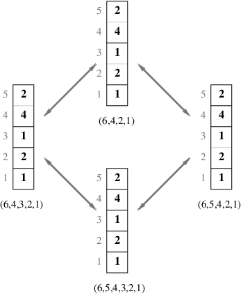
Figure 3. The towers associated to all 6-signatures. The second tower for instance, has blocks at positions 1, 2, and 4. The rightmost signature is the canonical one.
Refer to caption
Figure 4. The 5-signature (5,3,2,1)(5,3,2,1) has six associated arrays: The block at position 2 can hold either a 1 or a 2, while the block at position 3 can hold any descending combination of the numbers 1,2,31,2,3.
Lemma 4.

Let σ=(n,bs,…,b1){\sigma}=(n,b_{s},\ldots,b_{1}) be an nn-signature. Then

  1. (a)

    The number of nn-arrays associated to σ{\sigma} is (bsn−bs)​…​(b11){\textstyle\binom{b_{s}}{n-b_{s}}}\ldots{\textstyle\binom{b_{1}}{1}}.

  2. (b)

    The number of canonical nn-arrays is (n−1)!(n-1)!

  3. (c)

    The total number of nn-arrays is given by formula (1) when x=1x=1.

Proof.

The tower associated to σ{\sigma} has ss blocks. The jthj^{\rm th} block is based at position bjb_{j} and its length is bj+1−bjb_{j+1}-b_{j} (for the topmost block the length is n−bsn-b_{s}). Therefore the jthj^{\rm th} block can be filled with an arbitrary choice of bj+1−bjb_{j+1}-b_{j} numbers between 1 and bjb_{j}; i.e., (bjbj+1−bj){\textstyle\binom{b_{j}}{b_{j+1}-b_{j}}} possibilities. This proves (a), from which item (b) follows immediately. To prove (c), note from (3) that ana_{n} counts nn-arrays with weight xsx^{s}. Thus, when x=1x=1, ana_{n} simply counts the number of nn-arrays as claimed. ∎

Definition.

The sequence of numbers that specifies an array is called a pattern. We convene to read patterns from the bottom up; thus, for instance, the rightmost array in Figure 4 has pattern [1232][1232].

Lemma 5.

A tuple [t1,…,tn−1][t_{1},\ldots,t_{n-1}] is a valid pattern if and only if

tj≤j​ for all ​1≤j≤n−1.t_{j}\leq j\text{ for all }1\leq j\leq n-1.
Proof.

In a canonical array every block has length one. This means that the position of the jthj^{\rm th} block is bj=jb_{j}=j, and the number in this block is tjt_{j}. Thus, in this case, the pattern condition is equivalent to tj≤bj=jt_{j}\leq b_{j}=j, proving the result for canonical arrays.

In a non-canonical array, the cell at position jj belongs to a block at position i≤ji\leq j. The pattern condition states that the number tjt_{j} in that cell must be at most ii, and the result follows. ∎

3.3. Array Hypercubes

Definition.

If an array has a block at position pp with more than one cell, the block can be split into two shorter blocks. The result is a valid array since the blocks have positions pp and p+η>pp+\eta>p (η\eta is the location of the split within the original block), and the numbers in both blocks are all at most pp. We call this operation on arrays a split. Note that an array can usually be split in several ways, all of which commute. Moreover, repeated splitting eventually results in a canonical array.

The reverse operation is also well defined. If an array has two consecutive blocks at positions pp and p+ηp+\eta, and the numbers contained in both blocks run together in descending order, the two blocks can be combined into a single one. This is because the new block is at position pp and contains numbers in descending order, which means that the length of the new block cannot exceed its position. In other words, condition (4) is satisfied. This operation on arrays is called a merge. As with splitting, merge operations are commutative, and repeated merging must terminate. An array where no pair of blocks can be merged is called primitive.

Definition.

The graph 𝒢n{\mathcal{G}}_{n} on the set of nn-arrays is defined by joining any two arrays related by a single split/merge operation. Arrays belong to the same connected component of 𝒢n{\mathcal{G}}_{n} when they have the same pattern of numbers (disregarding block divisions). Note that a split/merge is possible at a given position if and only if the numbers at that position are in descending order. In particular, splitting/merging does not depend on the structure of blocks in an array, but only on the pattern of numbers. This yields the following lemma.

Lemma 6.

Every connected component of GnG_{n} is homeomorphic to a hypercube graph.

Proof.

Consider an array A∈𝒢nA\in{\mathcal{G}}_{n}. The connected component 𝒞{\mathcal{C}} of AA consists of all arrays with the same pattern of numbers as AA. This pattern has ℓ\ell descents (locations where the numbers are in descending order). Now view such locations as placeholders for a symbol 𝟣{\sf 1} or 𝟢{\sf 0} depending on whether two blocks of AA meet at that location or not. This puts the arrays of 𝒞{\mathcal{C}} in correspondence with vertices of the hypercube graph ℋℓ\mathcal{H}_{\ell}; see Figure 5. Since a split/merge depends only on the pattern of numbers, all edges of ℋℓ\mathcal{H}_{\ell} are included and 𝒞{\mathcal{C}} is homeomorphic to ℋℓ\mathcal{H}_{\ell}. ∎

Observation.

Every hypercube 𝒞⊂𝒢n{\mathcal{C}}\subset{\mathcal{G}}_{n} has a unique primitive array and a unique canonical array. In particular, the numbers of hypercubes in 𝒢n{\mathcal{G}}_{n} and of primitive nn-arrays are both equal to (n−1)!(n-1)! Also, if ℓ\ell is as in the proof above, the primitive array has s=n−ℓ−1s=n-\ell-1 blocks (because the canonical array has n−1n-1), so 𝒞{\mathcal{C}} is homeomorphic to ℋn−s−1\mathcal{H}_{n-s-1}.

Refer to caption
Figure 5. The pattern [12142][12142] has 2 descents, and thus determines four 6-arrays connected by split/merge operations into a square ℋ2\mathcal{H}_{2}.

4. The First Proofs

Each ana_{n} is a polynomial in xx. When written with the monomials ξr​xr\xi_{r}x^{r} in ascending order by degree, we say ana_{n} is in basic format. Since every nn-array with r−1r-1 blocks contributes xrx^{r} to the total ana_{n}, the coefficient ξr\xi_{r} counts the number of such arrays.

Example.

The first few ana_{n} in basic format are (compare (2)):

a1\displaystyle a_{1} =x,\displaystyle=x,
a2\displaystyle a_{2} =x2,\displaystyle=x^{2},
a3\displaystyle a_{3} =2​x3,\displaystyle=2x^{3},
a4\displaystyle a_{4} =x3+6​x4,\displaystyle=x^{3}+6x^{4},
a5\displaystyle a_{5} =10​x4+24​x5,\displaystyle=10x^{4}+24x^{5},
(5) a6\displaystyle a_{6} =8​x4+86​x5+120​x6.\displaystyle=8x^{4}+86x^{5}+120x^{6}.

When n=6n=6 for instance, we know that the towers with 4 blocks correspond to the three signatures (6,4,3,2,1)(6,4,3,2,1), (6,5,3,2,1)(6,5,3,2,1), and (6,5,4,2,1)(6,5,4,2,1) (see Figure 3). These have (42)​(31)​(21)​(11)=36{\textstyle\binom{4}{2}}{\textstyle\binom{3}{1}}{\textstyle\binom{2}{1}}{\textstyle\binom{1}{1}}=36, (51)​(32)​(21)​(11)=30{\textstyle\binom{5}{1}}{\textstyle\binom{3}{2}}{\textstyle\binom{2}{1}}{\textstyle\binom{1}{1}}=30, and (51)​(41)​(22)​(11)=20{\textstyle\binom{5}{1}}{\textstyle\binom{4}{1}}{\textstyle\binom{2}{2}}{\textstyle\binom{1}{1}}=20 associated arrays respectively, and we see that each of these 86 arrays contributes x5x^{5} to the value of a6a_{6}.

Recall that the array graph 𝒢n{\mathcal{G}}_{n} consists of isolated hypercube components. We can also break ana_{n} down as a sum of contributions by hypercubes. Let AA be a primitive nn-array with s=r−1s=r-1 blocks. We know that AA contributes xrx^{r} to ana_{n}. Since the connected component 𝒞{\mathcal{C}} of 𝒢{\mathcal{G}} containing AA is homeomorphic to ℋn−r\mathcal{H}_{n-r}, items (H2) and (H4) in Section 2.1 give

(6) ∑a∈𝒞x(#​blocks of ​a)+1=(H2)∑j=0n−r(n−rj)​xr+j=(H4)xr​(1+x)n−r.\sum_{a\in{\mathcal{C}}}x^{(\#\text{blocks of }a)+1}\stackrel{{\scriptstyle\eqref{item:HC-Stratification}}}{{=}}\sum_{j=0}^{n-r}{\displaystyle\binom{n-r}{j}}x^{r+j}\stackrel{{\scriptstyle\eqref{item:HC-Binomial}}}{{=}}x^{r}(1+x)^{n-r}.

Let primn​(r)\text{prim}_{n}(r) be the number of primitive arrays with r−1r-1 blocks; this is also the number of components of 𝒢n{\mathcal{G}}_{n} homeomorphic to ℋn−r\mathcal{H}_{n-r}. Equation (6) shows that the total contribution to ana_{n} of all arrays in all such hypercubes is primn​(r)⋅xr​(1+x)n−r\text{prim}_{n}(r)\cdot x^{r}(1+x)^{n-r}, so

(7) an=∑r=⌈log2⁡n⌉nprimn​(r)⋅xr​(1+x)n−ra_{n}=\sum_{r=\left\lceil\log_{2}n\right\rceil}^{n}\text{prim}_{n}(r)\cdot x^{r}(1+x)^{n-r}

(Condition (4) implies that the least possible number of blocks is ⌈log2⁡n⌉\left\lceil\log_{2}n\right\rceil).

When ana_{n} is written in that form, we can read that each of the primn​(r)\text{prim}_{n}(r) components of 𝒢n{\mathcal{G}}_{n} with dimension n−rn-r contributes xr​(1+x)n−rx^{r}(1+x)^{n-r} to the total sum ana_{n}. We will say that ana_{n} is in binomial format.

Example.

Let us compute the binomial format of a6a_{6}. From (5) we see that there are 8 arrays with 3 blocks. All of these must be primitive, so prim6​(4)=8\text{prim}_{6}(4)=8. These arrays (together with those obtained by splitting) determine 8 copies of ℋ2\mathcal{H}_{2} in 𝒢6{\mathcal{G}}_{6}. Gathering the monomials of all arrays in these hypercubes gives

a6=8​x4+86​x5+120​x6=(8​x4+16​x5+8​x6)+70​x5+112​x6=8​x4​(1+x)2+70​x5+112​x6.a_{6}=8x^{4}+86x^{5}+120x^{6}=\\ (8x^{4}+16x^{5}+8x^{6})+70x^{5}+112x^{6}=\\ 8x^{4}(1+x)^{2}+70x^{5}+112x^{6}.

The remaining 70 arrays with 4 blocks must be primitive since they do not belong to an ℋ2\mathcal{H}_{2}; i.e., prim6​(5)=70\text{prim}_{6}(5)=70. These arrays (together with those obtained by splitting) determine 70 copies of ℋ1\mathcal{H}_{1} in 𝒢6{\mathcal{G}}_{6}. Thus,

8​x4​(1+x)2+70​x5+112​x6=8​x4​(1+x)2+70​x5​(1+x)1+42​x6.8x^{4}(1+x)^{2}+70x^{5}+112x^{6}=8x^{4}(1+x)^{2}+70x^{5}(1+x)^{1}+42x^{6}.

The first few ana_{n} in binomial format are:

a1\displaystyle a_{1} =x1​y0,\displaystyle=x^{1}y^{0},
a2\displaystyle a_{2} =x2​y0,\displaystyle=x^{2}y^{0},
a3\displaystyle a_{3} =2​x3​y0,\displaystyle=2x^{3}y^{0},
a4\displaystyle a_{4} =x3​y1+5​x4​y0,\displaystyle=x^{3}y^{1}+5x^{4}y^{0},
a5\displaystyle a_{5} =10​x4​y1+14​x5​y0,\displaystyle=10x^{4}y^{1}+14x^{5}y^{0},
a6\displaystyle a_{6} =8​x4​y2+70​x5​y1+42​x6​y0,\displaystyle=8x^{4}y^{2}+70x^{5}y^{1}+42x^{6}y^{0},

where yy stand for 1+x1+x. This convetion makes for cleaner looking expressions, and will be consistently used in the rest of the paper.

Now that the combinatorial structure is in place, the proofs of Theorem 2 and the case x∉[−1,0]x\notin[-1,0] of Theorem 1 are straightforward.

Proof of Theorem 2.

Since x=−1x=-1, the only non-zero term in (7) occurs when r=nr=n. In other words,

an=(−1)n​primn​(n).a_{n}=(-1)^{n}\text{prim}_{n}(n).

Now, primn​(n)\text{prim}_{n}(n) is the number of nn-arrays with n−1n-1 blocks; that is, arrays that are both primitive and canonical. By definition, these are arrays with non-decreasing patterns of n−1n-1 numbers. Any such pattern can be associated to a monotone lattice path from (0,0)(0,0) to (n−1,n−1)(n-1,n-1) that does not cross over the diagonal. Simply substract 1 from each entry in the pattern and interpret the results as heights of the horizontal steps of a monotone path (compare Figure 2). This procedure is bijective, so by Lemma 3, primn​(n)=Cn\text{prim}_{n}(n)=C_{n}. ∎

Proof of Theorem 1 when x∉[−1,0]x\notin[-1,0].

Depending on the sign of xx, one of the two formats for ana_{n} displays no cancellations.

x>0x>0: All monomials ξr​xr\xi_{r}x^{r} in the basic format of ana_{n} are positive because the coefficient ξr\xi_{r} counts arrays with r−1r-1 blocks. In particular, ana_{n} is larger than the highest order monomial. The coefficient of this monomial is the number of arrays with the most blocks; i.e., canonical arrays. By Lemma 4,

an>(n−1)!⋅xn.a_{n}>(n-1)!\cdot x^{n}.

x<−1x<-1: Since y<0y<0, all terms primn​(r)⋅xr​yn−r\text{prim}_{n}(r)\cdot x^{r}y^{n-r} in the binomial format of ana_{n} have the same sign, and do not cancel each other. Also, |x|>|y||x|>|y|, so

|an|=∑rprimn​(r)⋅|xr​yn−r|>∑rprimn​(r)⋅|yn|=(n−1)!⋅|yn|,|a_{n}|=\sum_{r}\text{prim}_{n}(r)\cdot|x^{r}y^{n-r}|>\sum_{r}\text{prim}_{n}(r)\cdot|y^{n}|=(n-1)!\cdot|y^{n}|,

where the last equality follows from the observation after Lemma 6.

In both cases, |an||a_{n}| is larger than (n−1)!⋅wn(n-1)!\cdot w^{n} for some positive ww, and the result holds. ∎

5. The case x∈(−1,0)x\in(-1,0)

The situation when x∈(−1,0)x\in(-1,0) is more delicate because the terms in both the basic and binomial formats of ana_{n} have alternating signs. Our strategy in this second part involves a different representation ((8) and (9)) of ana_{n}. We will interpret the sequences {Sn​(1),…​Sn​(n−1)}\{S_{n}(1),\ldots S_{n}(n-1)\} as functions sn∈L2​[0,1]s_{n}\in L^{2}[0,1] and the recursion (9) as a sequence of integral operators An:sn↦sn+1A_{n}:s_{n}\mapsto s_{n+1}. We will deduce some facts about the shape of the graph of sns_{n}, and about the limit operator T=limAnT=\lim A_{n}. Then we will use this information to show that the largest eigenvalue λ{\lambda} of TT bounds from below the exponential rate of decay of an/(n−2)!a_{n}/(n-2)!

5.1. A new recursion

So far we have established that ana_{n} is the sum of contributions of the form xrx^{r} over a large set of arrays (for each array, r−1r-1 is the number of blocks). We grouped arrays with the same number pattern into hypercube graphs, and showed that ana_{n} is the sum of contributions xn−ℓ​(1+x)ℓ=xn−ℓ​yℓx^{n-\ell}(1+x)^{\ell}=x^{n-\ell}y^{\ell} over hypercubes 𝒞{\mathcal{C}}, where ℓ\ell is the dimension of each 𝒞{\mathcal{C}}. This dimension is the number of descents in the associated pattern, so we can abandon arrays and express ana_{n} directly as a sum of contributions over patterns:

an=∑ℓ=0n−⌈log2⁡n⌉−1∑patterns withℓ descentsxn−ℓ​yℓ.a_{n}=\sum_{\ell=0}^{n-\left\lceil\log_{2}n\right\rceil-1}\sum_{\begin{subarray}{c}\text{patterns with}\\ \text{$\ell$ descents}\end{subarray}}x^{n-\ell}y^{\ell}.

This allows us to sort the contributions to ana_{n} made by individual patterns. To this end, consider an nn-pattern π=[t1,…,tn−1]\pi=[t_{1},\ldots,t_{n-1}]. If the truncated pattern [t1,…,tn−2][t_{1},\ldots,t_{n-2}] contributes xa​ybx^{a}y^{b} to an−1a_{n-1}, then π\pi contributes xa​yb+1x^{a}y^{b+1} or xa+1​ybx^{a+1}y^{b} to ana_{n} depending on whether tn−1<tn−2t_{n-1}<t_{n-2} or not (i.e., on whether π\pi has one extra descent or not at the last position). This motivates the following definition.

Definition.

For n≥2n\geq 2 let Sn​(r)S_{n}(r) denote the sum of contributions of all patterns [t1,…,tn−1][t_{1},\ldots,t_{n-1}] such that tn−1t_{n-1} equals rr (thus, rr can take values in {1,…,n−1}\{1,\ldots,n-1\}). In particular, S2​(1)=x2S_{2}(1)=x^{2}, and

(8) an=∑j=1n−1Sn​(j).a_{n}=\sum_{j=1}^{n-1}S_{n}(j).

By the previous argument, Sn+1​(r)S_{n+1}(r) can be computed from the contributions of nn-patterns:

(9) Sn+1​(r)=x⋅∑j=1rSn​(j)+y⋅∑j=r+1n−1Sn​(j).S_{n+1}(r)=x\cdot\sum_{j=1}^{r}S_{n}(j)+y\cdot\sum_{j=r+1}^{n-1}S_{n}(j).

(when r=n−1r=n-1 or nn, there is no descent in the last position, so (9) should be interpreted to mean Sn+1​(n−1)=Sn+1​(n)=x⋅∑j=1n−1Sn​(j)S_{n+1}(n-1)=S_{n+1}(n)=x\cdot\sum_{j=1}^{n-1}S_{n}(j)).

Refer to caption
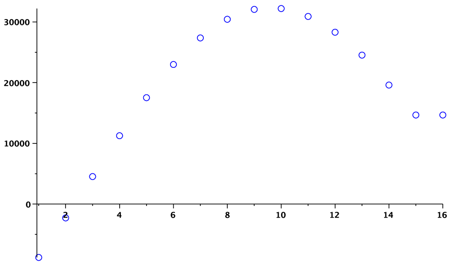
Figure 6.

Figure 6 shows a plot of the values {S16​(1),…,S16​(15)}\{S_{16}(1),\ldots,S_{16}(15)\} when x=−1/2x=-1/2. It is not coincidental that the graph looks sinusoidal.

5.2. Sinusoidal shape of 𝑺𝒏S_{n}

Note that

(10) Sn+1​(r)=Sn+1​(r−1)−Sn​(r).S_{n+1}(r)=S_{n+1}(r-1)-S_{n}(r).

From this relation we can derive a more convenient method of computing the sequence SnS_{n}:

  • •

    S2​(1)=x2S_{2}(1)=x^{2}; and for n≥3n\geq 3,

  • •

    Sn​(0)=y​∑j=1n−2Sn−1​(j)S_{n}(0)=y\sum_{j=1}^{n-2}S_{n-1}(j),

  • •

    Sn​(r)=Sn​(r−1)−Sn−1​(r),(1≤r≤n−2)S_{n}(r)=S_{n}(r-1)-S_{n-1}(r),\ (1\leq r\leq n-2),

  • •

    Sn​(n−1)=Sn​(n−2)S_{n}(n-1)=S_{n}(n-2).

Observation.

Sn​(0)S_{n}(0) is not part of the original sequence, but we will find it easier to study the properties of SnS_{n} by including this auxiliary term in the discussion. For instance, note that Sn​(0)=y​an−1S_{n}(0)=ya_{n-1} and Sn​(n−1)=x​an−1S_{n}(n-1)=xa_{n-1}. Recall that y=1+xy=1+x and x∈(−1,0)x\in(-1,0). It is vital to the coming arguments that these two values have opposite signs.

Definition.

The sequence SnS_{n} has

  • •

    a sign change if n≥4n\geq 4 and there are a,ba,b (1≤a<b≤n−21\leq a<b\leq n-2) such that

    Sn​(a)<0=Sn​(a+1)=…=Sn​(b−1)<Sn​(b)​ (an up-change) orSn​(a)>0=Sn​(a+1)=…=Sn​(b−1)>Sn​(b)​ (a down-change),\begin{array}[]{rcccl}S_{n}(a)&<&0=S_{n}(a+1)=\ldots=S_{n}(b-1)&<&S_{n}(b)\text{ (an {up-change}) or}\\ S_{n}(a)&>&0=S_{n}(a+1)=\ldots=S_{n}(b-1)&>&S_{n}(b)\text{ (a {down-change})},\end{array}
  • •

    an extreme if n≥5n\geq 5 and there are a,ba,b (0<a<b−1≤n−30<a<b-1\leq n-3) such that

    Sn​(a)<Sn​(a+1)=…=Sn​(b−1)>Sn​(b)​ (a maximum) orSn​(a)>Sn​(a+1)=…=Sn​(b−1)<Sn​(b)​ (a minimum),\begin{array}[]{rcccl}S_{n}(a)&<&S_{n}(a+1)=\ldots=S_{n}(b-1)&>&S_{n}(b)\text{ (a {maximum}) or}\\ S_{n}(a)&>&S_{n}(a+1)=\ldots=S_{n}(b-1)&<&S_{n}(b)\text{ (a {minimum})},\end{array}
  • •

    an inflection if n≥6n\geq 6 and there are a,ba,b (1≤a<b−2≤n−41\leq a<b-2\leq n-4) such that

    0<Sn−1​(a+1)<Sn−1​(a+2)=…=Sn−1​(b−1)>Sn−1​(b)>0​ or0>Sn−1​(a+1)>Sn−1​(a+2)=…=Sn−1​(b−1)<Sn−1​(b)<0.\begin{array}[]{rcccl}0<S_{n-1}(a+1)&<&S_{n-1}(a+2)=\ldots=S_{n-1}(b-1)&>&S_{n-1}(b)>0\text{ or}\\ 0>S_{n-1}(a+1)&>&S_{n-1}(a+2)=\ldots=S_{n-1}(b-1)&<&S_{n-1}(b)<0.\end{array}

The pair (a,b)(a,b) is the locus of the change/extreme/inflection. We also say that the change/extreme/inflection is located at aa.

Observation.

Recall that Sn−1​(c)=Sn​(c+1)−Sn​(c)S_{n-1}(c)=S_{n}(c+1)-S_{n}(c), so this value acts as a “discrete derivative” of the sequence SnS_{n} in the definition of inflection. Notice that in our inflections the slope at the center is steeper than at the sides. A corollary of property (ShB) below is that no other inflection shape is necessary. Also, note that Sn​(n−1)S_{n}(n-1) is not allowed to be part of a change/extreme/inflection.

Proposition 7.

For all n≥6n\geq 6 the sequence SnS_{n} satisfies

  1. (ShA)

    There are exactly one sign change, one extreme, and one inflection.

  2. (ShB)

    A maximum must have positive value and a minimum must have negative value.

  3. (ShC)

    There is at most one rr such that Sn​(r)=0S_{n}(r)=0.

  4. (ShD)

    At least one of the two values minr⁡Sn​(r)\min_{r}S_{n}(r) and maxr⁡Sn​(r)\max_{r}S_{n}(r) lies between x​anxa_{n} and y​anya_{n}.

  5. (ShE)

    If the extreme has locus (a,b)(a,b) and the inflection has locus (c,d)(c,d), then

    1. (a)

      a≤c⟹Sn−1​(0)<Sn−1​(1)<Sn−1​(2)<0a\leq c\Longrightarrow S_{n-1}(0)<S_{n-1}(1)<S_{n-1}(2)<0,

    2. (b)

      a>c⟹0>Sn−1​(0)>Sn−1​(1)>Sn−1​(2)a>c\Longrightarrow 0>S_{n-1}(0)>S_{n-1}(1)>S_{n-1}(2).

Refer to caption
Figure 7. The first row of pictures illustrates property (ShA) of Proposition 7. (1): at least one zero. (2): at most one zero. (3): at most one extreme. (4): at least one inflection. The second row illustrates properties (ShB), (ShC), (ShD), and (ShE).
Proof of (ShA).

A sign change in SnS_{n} implies an extreme in Sn+1S_{n+1}, which in turn implies an inflection in Sn+2S_{n+2}; therefore we only need to prove that SnS_{n} has exactly one sign change.

For n≥4n\geq 4, Sn​(0)=y​an−1S_{n}(0)=ya_{n-1} and Sn​(n−2)=x​an−1S_{n}(n-2)=xa_{n-1}. Since xx and yy have opposite signs, the sequence SnS_{n} has at least one sign change. If there were more changes than one, there would be at least three because sgn​(Sn​(0))≠sgn​(Sn​(n−2))\text{sgn}\big(S_{n}(0)\big)\neq\text{sgn}\big(S_{n}(n-2)\big). Then SnS_{n} has two extremes, and thus Sn−1S_{n-1} has two sign changes. But S4​(2)=S4​(3)S_{4}(2)=S_{4}(3), so S4S_{4} can have at most one sign change, so by induction, SnS_{n} has exactly one sign change. ∎

Proof of (ShB).

Assume Sn​(n−1)>0S_{n}(n-1)>0 (the negative case is analogous). In particular, a maximum of SnS_{n} must lie above Sn​(n−1)S_{n}(n-1) and thus be positive. Also, Sn​(0)=y​an−1<0S_{n}(0)=ya_{n-1}<0 because Sn​(n−1)=x​an−1S_{n}(n-1)=xa_{n-1}.

  • ∘\circ

    If Sn​(1)<0S_{n}(1)<0, then a minimum must lie lower than Sn​(1)S_{n}(1) and thus be negative.

  • ∘\circ

    If Sn​(1)>0S_{n}(1)>0, then there is an increase from Sn​(0)S_{n}(0), so Sn−1​(1)<0S_{n-1}(1)<0. Thus Sn−1S_{n-1} cannot have a down-change, and therefore SnS_{n} cannot have a minimum. ∎

Proof of (ShC).

Since SnS_{n} has at most one sign change, we need only discard the possibility of two (or more) consecutive zeros. Accordingly, assume that Sn​(r)=…=Sn​(r+k)=0S_{n}(r)=\ldots=S_{n}(r+k)=0 (k≥1k\geq 1) with Sn​(r−1)<0S_{n}(r-1)<0 and Sn​(r+k+1)≠0S_{n}(r+k+1)\neq 0 (the case Sn​(r−1)>0S_{n}(r-1)>0 is analogous).

Now, Sn​(r+k+1)<0S_{n}(r+k+1)<0 contradicts (ShB), so we can assume Sn​(r+k+1)>0S_{n}(r+k+1)>0. But then

Sn−1​(r)<0=Sn−1​(r+1)=…=Sn−1​(r+k)>Sn−1​(r+k+1),S_{n-1}(r)<0=S_{n-1}(r+1)=\ldots=S_{n-1}(r+k)>S_{n-1}(r+k+1),

and this means that Sn−1S_{n-1} contradicts (ShB). ∎

Proof of (ShD).

Assume Sn−1​(1)<0S_{n-1}(1)<0 so Sn​(1)>y​an−1S_{n}(1)>ya_{n-1} (the case Sn−1​(1)>0S_{n-1}(1)>0 is analogous). Moreover, Sn−1S_{n-1} cannot have a down-change (because it starts with a negative value); therefore SnS_{n} cannot have a minimum. Since SnS_{n} starts above y​an−1ya_{n-1} and ends at x​an−1xa_{n-1}, the conclusion follows. ∎

Proof of (ShE).

We can assume that the extreme of SnS_{n} is a maximum (the minimum case is analogous). Then Sn−1S_{n-1} has an up-change at (a+1,b)(a+1,b), and an extreme at (c+1,d)(c+1,d).

  1. (a)

    If a≤ca\leq c, Sn−1S_{n-1} has an increase (namely the up-change) before its extreme. Hence the extreme is a maximum which, therefore, lies above x​an−2xa_{n-2}. By (ShD),

    Sn−1​(0)=y​an−2≤Sn−1​(1)≤Sn−1​(2)<0.S_{n-1}(0)=ya_{n-2}\leq S_{n-1}(1)\leq S_{n-1}(2)<0.
  2. (b)

    If a>ca>c, Sn−1S_{n-1} has an increase (namely the up-change) after its extreme. Hence the extreme is a minimum which, therefore, lies below y​an−2ya_{n-2}. In particular, Sn−1S_{n-1} is decreasing until this minimum. We claim that it is decreasing starting at the auxiliary term, i.e., that Sn−1​(0)≥Sn−1​(1)S_{n-1}(0)\geq S_{n-1}(1); otherwise, Sn−2S_{n-2} has two sign changes. Then we have

    0>y​an=Sn−1​(0)≥Sn−1​(1)≥Sn−1​(2).∎0>ya_{n}=S_{n-1}(0)\geq S_{n-1}(1)\geq S_{n-1}(2).\qed

5.3. 𝑺𝒏S_{n} becomes a step function

Formula (9) induces a linear operator 𝑨n:ℝn−1⟶ℝn\mbox{\boldmath{$A$}}_{n}:\mathbb{R}^{n-1}\longrightarrow\mathbb{R}^{n}. Here we will embed 𝑨n\mbox{\boldmath{$A$}}_{n} as an integral operator An:L2​[0,1]⟶L2​[0,1]A_{n}:L^{2}[0,1]\longrightarrow L^{2}[0,1], and find an operator TT which is the limit of {An}\{A_{n}\} in the operator norm. The goal will be to link the growth of {an}\{a_{n}\} to the spectral properties of TT.

For n≥2n\geq 2, the rthr^{\rm th} entry of the column vector

𝒔n=[Sn(1)/(n−2)!⋮Sn(n−1)/(n−2)!]∈ℝn−1\mbox{\boldmath{$s$}}_{n}=\left[\begin{tabular}[]{c}$S_{n}(1)/(n-2)!$\\ $\vdots$\\ $S_{n}(n-1)/(n-2)!$\end{tabular}\right]\in\mathbb{R}^{n-1}

represents the average contribution to ana_{n} of patterns with last entry tn−1=rt_{n-1}=r (of which there are (n−2)!(n-2)!). With this notation, Equation (9) can be interpreted as a linear transformation

(11) 𝒔n+1=(𝑨n⋅𝒔n)/(n−1),\mbox{\boldmath{$s$}}_{n+1}=(\mbox{\boldmath{$A$}}_{n}\cdot\mbox{\boldmath{$s$}}_{n})/(n-1),

where 𝑨n\mbox{\boldmath{$A$}}_{n} is the n×(n−1)n\times(n-1) matrix whose (i,j)(i,j)-entry is xx if i≥ji\geq j, and yy otherwise.

Let En:ℝn−1⟶L2​[0,1]E_{n}:\mathbb{R}^{n-1}\longrightarrow L^{2}[0,1] be the linear map that sends the standard basis vector 𝒆j\mbox{\boldmath{$e$}}_{j} to the characteristic function of the interval [j−1n−1,jn−1)\left[\frac{j-1}{n-1},\frac{j}{n-1}\right). The vector 𝒔n\mbox{\boldmath{$s$}}_{n} maps to the step function sn=En​(𝒔n)s_{n}=E_{n}(\mbox{\boldmath{$s$}}_{n}), such that sn​(u)=Sn​(j)/(n−2)!s_{n}(u)=S_{n}(j)/(n-2)! whenever u∈[j−1n−1,jn−1)u\in\left[\frac{j-1}{n-1},\frac{j}{n-1}\right). The maps {En}\{E_{n}\} embed the linear operators 𝑨n:ℝn−1⟶ℝn\mbox{\boldmath{$A$}}_{n}:\mathbb{R}^{n-1}\longrightarrow\mathbb{R}^{n} into linear operators An:L2​[0,1]⟶L2​[0,1]A_{n}:L^{2}[0,1]\longrightarrow L^{2}[0,1]. In particular, Equation (11) takes the form

(12) sn+1​(u)=[An​(sn)]​(u)=∫01αn​(u,v)⋅sn​(v)​𝑑v,s_{n+1}(u)=\left[A_{n}(s_{n})\right](u)=\int_{0}^{1}\alpha_{n}(u,v)\cdot s_{n}(v)\;{\rm d}v,

where the kernel αn\alpha_{n} is a piecewise constant function whose value at (u,v)∈[i−1n,in)×[j−1n−1,jn−1)(u,v)\in\left[\frac{i-1}{n},\frac{i}{n}\right)\times\left[\frac{j-1}{n-1},\frac{j}{n-1}\right) is

αn​(u,v)={x if ​i≥jy otherwise(i.e., equal to ​(𝑨n)i​j).\alpha_{n}(u,v)=\begin{cases}x&\text{ if }i\geq j\\ y&\text{ otherwise}\end{cases}\qquad\big(\text{i.e., equal to }(\mbox{\boldmath{$A$}}_{n})_{ij}\big).
Observation.

The factor 1/(n−1)1/(n-1) in (11) is hidden as a normalization factor in (12). Indeed, when uu lies in the interval [i−1n,in)\left[\frac{i-1}{n},\frac{i}{n}\right),

[An​(sn)]​(u)=\displaystyle\left[A_{n}(s_{n})\right](u)= ∫01αn​(u,v)⋅En​(𝒔n)​(v)​𝑑v=\displaystyle\int_{0}^{1}\alpha_{n}(u,v)\cdot E_{n}(\mbox{\boldmath{$s$}}_{n})(v)\;{\rm d}v=
∑j=1n−1∫[j−1n−1,jn−1)(𝑨n)i​j​Sn​(j)(n−2)!​𝑑v=\displaystyle\sum_{j=1}^{n-1}\int_{\left[\frac{j-1}{n-1},\frac{j}{n-1}\right)}(\mbox{\boldmath{$A$}}_{n})_{ij}\frac{S_{n}(j)}{(n-2)!}\;{\rm d}v=
∑j=1n−1(𝑨n)i​j​Sn​(j)(n−2)!⋅1n−1,\displaystyle\sum_{j=1}^{n-1}(\mbox{\boldmath{$A$}}_{n})_{ij}\frac{S_{n}(j)}{(n-2)!}\cdot\frac{1}{n-1},

which is the ithi^{\rm th} entry of 𝒔n+1\mbox{\boldmath{$s$}}_{n+1}. In particular, (compare equation (8)):

an=(n−1)!​∫01sn​(v)​𝑑v.a_{n}=(n-1)!\int_{0}^{1}s_{n}(v)\;{\rm d}v.

To prove the theorem we need to show that the rate of exponential decay of the integrals ∫01sn​(v)​𝑑v\int_{0}^{1}s_{n}(v)\;{\rm d}v is bounded from below. The bound will be dictated by the largest eigenvalue λ{\lambda} of the limit operator of AnA_{n}.

5.4. The limit operator 𝑻T

Here we define the limit operator TT of the sequence {An}\{A_{n}\}, and establish some of its basic properties.

Let T:L2​[0,1]⟶L2​[0,1]T:L^{2}[0,1]\longrightarrow L^{2}[0,1] by

(T​f)​(u)=∫01κ⁡(u,v)⋅f⁡(v)​𝑑v,(Tf)(u)=\int_{0}^{1}\kappa(u,v)\cdot f(v)\;{\rm d}v,

with kernel

κ⁡(u,v)={x if ​u≥vy otherwise.\kappa(u,v)=\begin{cases}x&\text{ if }u\geq v\\ y&\text{ otherwise}.\end{cases}
Lemma 8.

The operator TT is the limit of {An}\{A_{n}\} in the operator norm:

‖T−An‖≤1n.\left\|T-A_{n}\right\|\leq\frac{1}{\sqrt{n}}.
Refer to caption
Figure 8. The kernel α10\alpha_{10} (the shaded region is Ω10\Omega_{10}). Note that the unit square is divided into rectangles of size 110\frac{1}{10} by 19\frac{1}{9}.
Proof.

The kernel of T−AnT-A_{n} is the function κ−αn\kappa-\alpha_{n}. Since yy is just a shorthand for 1+x1+x, we see that κ−αn\kappa-\alpha_{n} is the characteristic function of the staircase region Ωn\Omega_{n} in the unit square, consisting of the upper triangle {0≤u,v≤1|u<v}\{0\leq u,v\leq 1\;|\;u<v\}, minus those rectangles [i−1n,in)×[j−1n−1,jn−1)\left[\frac{i-1}{n},\frac{i}{n}\right)\times\left[\frac{j-1}{n-1},\frac{j}{n-1}\right) such that i<ji<j. Then the Lebesgue measure of Ωn\Omega_{n} is

μ⁡(Ωn)=12−(n−2)​(n−1)2⋅1n⁡(n−1)=1n.\mu(\Omega_{n})=\frac{1}{2}-\frac{(n-2)(n-1)}{2}\cdot\frac{1}{n(n-1)}=\frac{1}{n}.

It follows that

‖T−An‖L2≤(μ⁡(Ωn))1/2=1n.∎\left\|T-A_{n}\right\|_{L^{2}}\leq\big(\mu(\Omega_{n})\big)^{1/2}=\frac{1}{\sqrt{n}}.\qed

5.5. Eigenfunctions of 𝑻T

The operator TT can be expressed as follows:

(T​f)​(u)=\displaystyle(Tf)(u)= ∫01κ⁡(u,v)⋅f⁡(v)​𝑑v=\displaystyle\int_{0}^{1}\kappa(u,v)\cdot f(v)\;{\rm d}v=
x⋅∫0uf⁡(v)​𝑑v+y⋅∫u1f⁡(v)​𝑑v=\displaystyle x\cdot\int_{0}^{u}f(v)\;{\rm d}v+y\cdot\int_{u}^{1}f(v)\;{\rm d}v=
−F⁡(u)+y⋅F⁡(1)−x⋅F⁡(0),\displaystyle-F(u)+y\cdot F(1)-x\cdot F(0),

where FF is any primitive of ff. To find the eigenvalues of TT, set

(13) (λ​f)​(u)=\displaystyle({\lambda}f)(u)= (T​f)​(u)=\displaystyle(Tf)(u)=
−F⁡(u)+y⋅F⁡(1)−x⋅F⁡(0),\displaystyle-F(u)+y\cdot F(1)-x\cdot F(0),

and differentiate to obtain the ODE

f′​(u)=−f⁡(u)λ,f^{\prime}(u)=\frac{-f(u)}{{\lambda}},

with general solution

f(u)=Ce−u/λ.f(u)=C{\rm e}^{-u/{\lambda}}.

A primitive of ff is F(u)=−λCe−u/λF(u)=-{\lambda}C{\rm e}^{-u/{\lambda}}, so substituting in (13) gives

λ(Ce−1/λ)=λCe−u/λ−λC(y⋅e−1/λ−x).{\lambda}\big(C{\rm e}^{-1/{\lambda}}\big)={\lambda}C{\rm e}^{-u/{\lambda}}-{\lambda}C\left(y\cdot{\rm e}^{-1/{\lambda}}-x\right).

Thus, λ{\lambda} is an eigenvalue if and only if

e−1/λ=xy.{\rm e}^{-1/{\lambda}}=\frac{x}{y}.

Note that xy<0\frac{x}{y}<0 exactly when x∈(−1,0)x\in(-1,0). Then we can write the eigenvalues as

λm=−1log⁡xy+2​m​π​i=−1log⁡|xy|+(2​m+1)​π​i​ for all ​m∈ℤ,{\lambda}_{m}=\frac{-1}{\log\frac{x}{y}+2m\pi{\rm i}}=\frac{-1}{\log\big|\frac{x}{y}\big|+(2m+1)\pi{\rm i}}\text{ for all }m\in\mathbb{Z},

and the eigenfunction corresponding to λm{\lambda}_{m} is

fm​(u)=|xy|u​e(2​m+1)​π​i​u.f_{m}(u)=\big|\tfrac{x}{y}\big|^{u}{\rm e}^{(2m+1)\pi{\rm i}u}.
Definition.

For ease of notation, we write the absolute values of the two largest eigenvalues as λ:=|λ−1|=|λ0|{\lambda}:=|{\lambda}_{-1}|=|{\lambda}_{0}| and μ:=|λ−2|=|λ1|\mu:=|{\lambda}_{-2}|=|{\lambda}_{1}|.

Lemma 9.

The family of functions {fm}m∈ℤ\{f_{m}\}_{m\in\mathbb{Z}} forms a basis of L2​[0,1]L^{2}[0,1].

Proof.

Let ff be an arbitrary function in L2​[0,1]L^{2}[0,1]. Since x∈(−1,0)x\in(-1,0), the function g⁡(u)=|yx|u​e−π​i​ug(u)=\big|\frac{y}{x}\big|^{u}{\rm e}^{-\pi{\rm i}u} is continuous, so f​g∈L2​[0,1]fg\in L^{2}[0,1]. After rescaling the standard basis of L2​[−π,π]L^{2}[-\pi,\pi], we obtain the representation

(f​g)​(u)=∑m∈ℤcm⋅e2​m​π​i​u,(fg)(u)=\sum_{m\in\mathbb{Z}}c_{m}\cdot{\rm e}^{2m\pi{\rm i}u},

which implies

f⁡(u)=∑m∈ℤcm⋅|xy|u​e(2​m+1)​π​i​u=∑m∈ℤcm⋅fm​(u).f(u)=\sum_{m\in\mathbb{Z}}c_{m}\cdot\big|\tfrac{x}{y}\big|^{u}{\rm e}^{(2m+1)\pi{\rm i}u}=\sum_{m\in\mathbb{Z}}c_{m}\cdot f_{m}(u).

The reverse argument shows that {fm}\{f_{m}\} are linearly independent. ∎

In order to turn {fm}\{f_{m}\} into an orthonormal basis, we introduce the weighted inner product

(14) ⟨f,g⟩=∫01|xy|−2​v​f​(v)​g¯​(v)​𝑑v.\langle f,g\rangle=\int_{0}^{1}\big|\tfrac{x}{y}\big|^{-2v}f(v)\overline{g}(v)\;{\rm d}v.

Note that for m≥0m\geq 0 the pair of functions f−(m+1),fmf_{-(m+1)},f_{m} are complex conjugate and their eigenvalues have the same magnitude. As a consequence, a convenient basis for the subspace Lℝ2​[0,1]⊂L2​[0,1]L_{\mathbb{R}}^{2}[0,1]\subset L^{2}[0,1] of real-valued functions is

{|xy|u​cos⁡((2​m+1)​π​u),|xy|u​sin⁡((2​m+1)​π​u)}m≥0.\left\{\big|\tfrac{x}{y}\big|^{u}\cos\big((2m+1)\pi u\big),\big|\tfrac{x}{y}\big|^{u}\sin\big((2m+1)\pi u\big)\right\}_{m\geq 0}.

6. The functional approach

In this section we establish the lower bound on the exponential rate of decay of the sequence an/(n−2)!a_{n}/(n-2)! The long proof of Lemma 10 interferes with the flow of logic, and is consequently deferred to the next section.

Definition.

The eigenfunctions f−1f_{-1} and f0f_{0} with largest eigenvalue λ{\lambda} span a complex two-dimensional subspace of L2​[0,1]L^{2}[0,1]. Let E⊂Lℝ2​[0,1]E\subset L_{\mathbb{R}}^{2}[0,1] denote the real slice of this subspace generated by {|xy|u​cos⁡(π​u),|xy|u​sin⁡(π​u)}\left\{\big|\tfrac{x}{y}\big|^{u}\cos\big(\pi u\big),\,\big|\tfrac{x}{y}\big|^{u}\sin\big(\pi u\big)\right\}. The space E⟂E^{\perp} spanned by all other eigenfunctions is orthogonal to EE, so that (by Lemma 9) Lℝ2​[0,1]=E⊕E⟂L_{\mathbb{R}}^{2}[0,1]=E\oplus E^{\perp}. The projections onto EE and E⟂E^{\perp} are denoted PP and P⟂P^{\perp} respectively. By Parseval’s Theorem we can define the angle θn\theta_{n} by any of the three equivalent formulas

sin⁡θn:=‖P⟂​sn‖2‖sn‖2,cos⁡θn:=‖P​sn‖2‖sn‖2,tan⁡θn:=‖P⟂​sn‖2‖P​sn‖2.\sin\theta_{n}:=\frac{\|P^{\perp}s_{n}\|_{2}}{\|s_{n}\|_{2}},\quad\cos\theta_{n}:=\frac{\|Ps_{n}\|_{2}}{\|s_{n}\|_{2}},\quad\tan\theta_{n}:=\frac{\|P^{\perp}s_{n}\|_{2}}{\|Ps_{n}\|_{2}}.

Intuitively, the closer θn\theta_{n} is to 00, the better sns_{n} resembles a function in EE.

Now we can describe the strategy of the proof:

  1. Step 1:

    We use the shape properties of the sequence SnS_{n} to show that the angles θn\theta_{n} are bounded away from π/2\pi/2.

  2. Step 2:

    The sequence {θn}\{\theta_{n}\} converges to 00, so the functions sns_{n} become progressively sinusoidal.

  3. Step 3:

    There is a sequence of indices {nk}\{n_{k}\} such that {|ank|}\{|a_{n_{k}}|\} is comparable to {‖snk‖2}\{\|s_{n_{k}}\|_{2}\}. Meanwhile, ‖sn‖2≥(λ−ε)n\|s_{n}\|_{2}\geq({\lambda}-\varepsilon)^{n} for arbitrarily small ε\varepsilon, and the result will follow.

6.1. Step 1 (𝜽𝒏≤𝚯<𝝅/𝟐)(\theta_{n}\leq\Theta<\pi/2)

Fix nn and consider the locus (a,b)(a,b) of the sign change of SnS_{n}. The value zn:=a/(n−1)∈[0,1)z_{n}:=a/(n-1)\in[0,1) is such that sn​(u)⋅sin⁡(π⁡(u−zn))s_{n}(u)\cdot\sin(\pi(u-z_{n})) never changes sign. We will show there is a K>0K>0 such that for all nn,

(15) |⟨sn(u),|xy|usinπ(u−zn⟩|>K∥sn∥2.\big|\langle s_{n}(u),\big|\tfrac{x}{y}\big|^{u}\sin\pi(u-z_{n}\rangle\big|>K\|s_{n}\|_{2}.

The projection P​snPs_{n} is larger than |⟨sn(u),|xy|usinπ(u−zn⟩||\langle s_{n}(u),\big|\tfrac{x}{y}\big|^{u}\sin\pi(u-z_{n}\rangle|, and thus the angle θn\theta_{n} is bounded away from π/2\pi/2 by

θn<arccos⁡K=:Θ<π/2.\theta_{n}<\arccos K=:\Theta<\pi/2.

The proof of (15) follows from Corollary 11 and Lemma 12 below, using K=C​C′K=CC^{\prime}.

Lemma 10.

The sequences {‖sn‖1}\{\|s_{n}\|_{1}\} and {‖sn‖∞}\{\|s_{n}\|_{\infty}\} are comparable in the sense that there is a constant CC such that for all nn,

‖sn‖∞≥‖sn‖1≥C​‖sn‖∞.\|s_{n}\|_{\infty}\geq\|s_{n}\|_{1}\geq C\|s_{n}\|_{\infty}.

This is the main technical lemma, and its proof is deferred to Section 7.

Corollary 11.

The sequences {‖sn‖1}\{\|s_{n}\|_{1}\} and {‖sn‖2}\{\|s_{n}\|_{2}\} are comparable in the sense that there is a constant CC such that for all nn,

‖sn‖2≥‖sn‖1≥C​‖sn‖2.\|s_{n}\|_{2}\geq\|s_{n}\|_{1}\geq C\|s_{n}\|_{2}.
Proof.

The left side is the Cauchy-Schwarz inequality. On the right we have

‖sn‖12≥C2​‖sn‖∞2≥C2​∫01sn2​(v)​𝑑v=C2​‖sn‖22.∎\|s_{n}\|_{1}^{2}\geq C^{2}\|s_{n}\|_{\infty}^{2}\geq C^{2}\int_{0}^{1}s_{n}^{2}(v)\;{\rm d}v=C^{2}\|s_{n}\|_{2}^{2}.\qed
Lemma 12.

Let znz_{n} be defined as above. Then there is a constant C′C^{\prime} such that

|⟨sn​(u),|xy|u​sin⁡π⁡(u−zn)⟩|>C′​‖sn‖1.\big|\langle s_{n}(u),\big|\tfrac{x}{y}\big|^{u}\sin\pi(u-z_{n})\rangle\big|>C^{\prime}\|s_{n}\|_{1}.
Proof.

Given z∈[0,1]z\in[0,1], the maximum of the function |xy|−u⋅|sin⁡π⁡(u−z)||\tfrac{x}{y}|^{-u}\cdot|\sin\pi(u-z)| in a small interval [z−ε,z+ε]∩[0,1][z-\varepsilon,z+\varepsilon]\cap[0,1] is Mz,ε>0M_{z,\varepsilon}>0; a quantity that varies continuously. Fix ε≡ε⁡(z)\varepsilon\equiv\varepsilon(z) so that the Lebesgue measure of the set

Lz:={u∈[0,1] s.t. |xy|−u⋅|sinπ(u−z)|<Mz,ε}L_{z}:=\{u\in[0,1]\text{ s.t. }|\tfrac{x}{y}|^{-u}\cdot|\sin\pi(u-z)|<M_{z,\varepsilon}\}

is C/2C/2, where CC is the constant of Lemma 10. This is well defined because |xy|−u⋅|sin⁡π⁡(u−z)||\tfrac{x}{y}|^{-u}\cdot|\sin\pi(u-z)| is nowhere constant, so the measure of LzL_{z} varies continuously. Since [0,1][0,1] is compact, the lower bound M:=infz∈[0,1]Mz,εM:=\inf_{z\in[0,1]}M_{z,\varepsilon} is positive.

Recall that znz_{n} is chosen so that sn​(u)⋅sin⁡π⁡(u−zn)s_{n}(u)\cdot\sin\pi(u-z_{n}) has constant sign. For simplicity, let us assume that this sign is positive. Then the weighted inner product |⟨sn​(u),|xy|u​sin⁡π⁡(u−zn)⟩|\big|\langle s_{n}(u),\big|\tfrac{x}{y}\big|^{u}\sin\pi(u-z_{n})\rangle\big| equals (compare (14)):

∫01|xy|−v​sn​(v)⋅sin⁡π⁡(v−zn)​𝑑v≥∫Lzn∁|xy|−v​sn​(v)⋅sin⁡π⁡(v−zn)​𝑑v>\displaystyle\int_{0}^{1}|\tfrac{x}{y}|^{-v}s_{n}(v)\cdot\sin\pi(v-z_{n})\;{\rm d}v\geq\int_{L_{z_{n}}^{\complement}}|\tfrac{x}{y}|^{-v}s_{n}(v)\cdot\sin\pi(v-z_{n})\;{\rm d}v>
M​∫Lzn∁|sn​(v)|​𝑑v=M⁡(∫01|sn​(v)|​𝑑v−∫Lzn|sn​(v)|​𝑑v).\displaystyle M\int_{L_{z_{n}}^{\complement}}|s_{n}(v)|\;{\rm d}v=M\left(\int_{0}^{1}|s_{n}(v)|\;{\rm d}v-\int_{L_{z_{n}}}|s_{n}(v)|\;{\rm d}v\right).

But

∫Lzn|sn​(v)|​𝑑v<μ⁡(Lzn)​‖sn‖∞=C2​‖sn‖∞<12​‖sn‖1\int_{L_{z_{n}}}|s_{n}(v)|\;{\rm d}v<\mu(L_{z_{n}})\|s_{n}\|_{\infty}=\tfrac{C}{2}\|s_{n}\|_{\infty}<\tfrac{1}{2}\|s_{n}\|_{1}

by Lemma 10, so we get

|⟨sn​(u),|xy|u​sin⁡π⁡(u−zn)⟩|>M2​‖sn‖1.∎\big|\langle s_{n}(u),\big|\tfrac{x}{y}\big|^{u}\sin\pi(u-z_{n})\rangle\big|>\tfrac{M}{2}\|s_{n}\|_{1}.\qed

6.2. Step 2 (𝜽𝒏→𝟎)(\theta_{n}\rightarrow 0)

We will show in Lemma 13 that when nn is large enough, the sequence {tan⁡θn}\{\tan\theta_{n}\} enters a decreasing regime that makes it eventually converge to 0. This establishes the desired result.

First we derive two versions of the basic estimate for tan⁡θn+1\tan\theta_{n+1}:

tan⁡θn+1=‖P⟂​An​sn‖2‖P​An​sn‖2=‖P⟂​[T​sn+(An−T)]‖2‖P⁡[T​sn+(An−T)]‖2≤‖P⟂​T​sn‖2+‖P⟂​(An−T)​sn‖2|‖P​T​sn‖2−‖P⁡(An−T)​sn‖2|,\tan\theta_{n+1}=\frac{\|P^{\perp}A_{n}s_{n}\|_{2}}{\|PA_{n}s_{n}\|_{2}}=\frac{\|P^{\perp}[Ts_{n}+(A_{n}-T)]\|_{2}}{\|P[Ts_{n}+(A_{n}-T)]\|_{2}}\leq\frac{\|P^{\perp}Ts_{n}\|_{2}+\|P^{\perp}(A_{n}-T)s_{n}\|_{2}}{\big|\|PTs_{n}\|_{2}-\|P(A_{n}-T)s_{n}\|_{2}\big|},

and that θn<Θ\theta_{n}<\Theta allows us to remove the absolute value in the denominator by assuming nn is large enough. Since TT commutes with the projections PP and P⟂P^{\perp}, and using Lemma 8,

tan⁡θn+1\displaystyle\tan\theta_{n+1} ≤μ​‖P⟂​sn‖2+‖sn‖2/nλ​‖P​sn‖2−‖sn‖2/n=\displaystyle\leq\frac{\mu\|P^{\perp}s_{n}\|_{2}+\|s_{n}\|_{2}/\sqrt{n}}{{\lambda}\|Ps_{n}\|_{2}-\|s_{n}\|_{2}/\sqrt{n}}=
(16) =nμsinθn+1nλcosθn−1\displaystyle=\frac{\sqrt{n}\mu\sin\theta_{n}+1}{\sqrt{n}{\lambda}\cos\theta_{n}-1}
(17) =(μ+1nsinθnλ−1ncosθn)tanθn.\displaystyle=\left(\frac{\mu+\frac{1}{\sqrt{n}\sin\theta_{n}}}{{\lambda}-\frac{1}{\sqrt{n}\cos\theta_{n}}}\right)\tan\theta_{n}.
Lemma 13.

Let n>9cos2⁡Θ​(λ−μ)2n>\frac{9}{\cos^{2}\Theta({\lambda}-\mu)^{2}}. Then there are constants 0<ε<10<\varepsilon<1 and R>0R>0 such that

  1. a)

    If nsinθn≥3λ−μ\sqrt{n}\sin\theta_{n}\geq\frac{3}{{\lambda}-\mu}, then

    tanθn+1<(1−ε)tanθn.\tan\theta_{n+1}<(1-\varepsilon)\tan\theta_{n}.
  2. b)

    If nsinθn≤3λ−μ\sqrt{n}\sin\theta_{n}\leq\frac{3}{{\lambda}-\mu}, then

    tan⁡θn+1<Rn.\tan\theta_{n+1}<\frac{R}{\sqrt{n}}.

In other words, when nn is sufficiently large, each step in the sequence {tan⁡θn}\{\tan\theta_{n}\} affords a definite relative decrease, or a slower but absolute decrease.

Proof of Lemma 13.


  1. a)

    The angle θn\theta_{n} is smaller than Θ\Theta, so the initial assumption on nn implies

    λ−1ncosθn>λ−1n​cos⁡Θ>λ−λ−μ3.{\lambda}-\frac{1}{\sqrt{n}\cos\theta_{n}}>{\lambda}-\frac{1}{\sqrt{n}\cos\Theta}>{\lambda}-\frac{{\lambda}-\mu}{3}.

    The condition nsinθn≥3λ−μ\sqrt{n}\sin\theta_{n}\geq\frac{3}{{\lambda}-\mu} is equivalent to

    μ+1nsinθn<μ+λ−μ3,\mu+\frac{1}{\sqrt{n}\sin\theta_{n}}<\mu+\frac{{\lambda}-\mu}{3},

    so (17) is smaller than

    (μ+λ−μ3λ−λ−μ3)tanθn=(2​μ+λ2​λ+μ)tanθn.\left(\frac{\mu+\frac{{\lambda}-\mu}{3}}{{\lambda}-\frac{{\lambda}-\mu}{3}}\right)\tan\theta_{n}=\left(\frac{2\mu+{\lambda}}{2{\lambda}+\mu}\right)\tan\theta_{n}.

    Since 2​μ+λ2​λ+μ<1\frac{2\mu+{\lambda}}{2{\lambda}+\mu}<1, this case is proved.

  2. b)

    When nsinθn≤3λ−μ\sqrt{n}\sin\theta_{n}\leq\frac{3}{{\lambda}-\mu}, we also have ncosθn≥n−9(λ−μ)2\sqrt{n}\cos\theta_{n}\geq\sqrt{n-\frac{9}{({\lambda}-\mu)^{2}}}. Substituting in (16) gives

    tan⁡θn+1<μ​3λ−μ+1λ​n−9(λ−μ)2−1,\tan\theta_{n+1}<\frac{\mu\frac{3}{{\lambda}-\mu}+1}{{\lambda}\sqrt{n-\frac{9}{({\lambda}-\mu)^{2}}}-1},

    and the result follows. ∎

6.3. Step 3 (|∫𝒔𝒏𝒌|>CLOSE(|\int s_{n_{k}}|> cst OPEN(𝝀−𝜺)𝒏𝒌)({\lambda}-\varepsilon)^{n_{k}})

We are ready to prove that

(18) |∫01sn​(v)​𝑑v|≥(λ−ε)n\left|\int_{0}^{1}s_{n}(v)\;{\rm d}v\right|\geq({\lambda}-\varepsilon)^{n}

along a subsequence of indices. The immediate consequence is factorial growth of |an||a_{n}|, since an=(n−2)!⋅∫01sn​(v)​𝑑va_{n}=(n-2)!\cdot\int_{0}^{1}s_{n}(v)\;{\rm d}v. Equation (18) follows at once from propositions 14 and 15.

Proposition 14.

There is an infinite integer sequence n1<n2<…n_{1}<n_{2}<\ldots, and a constant 0<W≤10<W\leq 1 such that for all kk,

|∫01snk​(v)​𝑑v|≥W17​‖snk‖2.\left|\int_{0}^{1}s_{n_{k}}(v)\;{\rm d}v\right|\geq\tfrac{W}{\sqrt{17}}\|s_{n_{k}}\|_{2}.
Proposition 15.

For every ε>0\varepsilon>0 there are constants G,N>0G,N>0 such that for n>Nn>N,

‖sn‖2>G​(λ−ε)n.\|s_{n}\|_{2}>G({\lambda}-\varepsilon)^{n}.

The proof of Proposition 14 uses the following auxiliary result:

Lemma 16.

There is an infinite integer sequence n1<n2<…n_{1}<n_{2}<\ldots such that for all kk,

(19) |∫01P​snk​(v)​𝑑v|≥12​∫01|P​snk​(v)|​𝑑v.\left|\int_{0}^{1}Ps_{n_{k}}(v)\;{\rm d}v\right|\geq\tfrac{1}{2}\int_{0}^{1}|Ps_{n_{k}}(v)|\;{\rm d}v.

We prove Lemma 16 first, and then propositions 14 and 15.

Proof of Lemma 16.

First notice that ∫01sin⁡(π⁡(u+ω))​𝑑v=2π​cos⁡π​ω\int_{0}^{1}\sin(\pi(u+\omega))\;{\rm d}v=\tfrac{2}{\pi}\cos\pi\omega, so

(20) ∫01sin⁡(π⁡(u+ω))​𝑑v≥12​∫01sin⁡(π​u)​𝑑v​ if and only if |ω⁡(mod​  1)|≤1/4.\int_{0}^{1}\sin(\pi(u+\omega))\;{\rm d}v\geq\tfrac{1}{\sqrt{2}}\int_{0}^{1}\sin(\pi u)\;{\rm d}v\text{ if and only if }|\omega\allowbreak\mkern 5.0mu({\operator@font mod}\,\,1)|\leq 1/4.

The lemma will follow once we prove that if a large enough nn does not satisfy (19), then n+1n+1 does. Accordingly, assume that

|∫01P​sn​(v)​𝑑v|≤12​∫01|P​sn​(v)|​𝑑v<12​∫01|P​sn​(v)|​𝑑v.\left|\int_{0}^{1}Ps_{n}(v)\;{\rm d}v\right|\leq\tfrac{1}{2}\int_{0}^{1}|Ps_{n}(v)|\;{\rm d}v<\tfrac{1}{\sqrt{2}}\int_{0}^{1}|Ps_{n}(v)|\;{\rm d}v.

Since the function P​snPs_{n} is in EE, it has the form P​sn​(u)=B​sin⁡(π⁡(u+ω))Ps_{n}(u)=B\sin(\pi(u+\omega)) for some constants BB, ω\omega. According to (20), the assumption above means that |ω⁡(mod​  1)|≥1/4|\omega\allowbreak\mkern 5.0mu({\operator@font mod}\,\,1)|\geq 1/4. Now,

(21) |∫01P​sn+1​(v)​𝑑v|=|∫01P​T​sn​(v)​𝑑v+∫01P⁡(An−T)​sn​(v)​𝑑v|.\left|\int_{0}^{1}Ps_{n+1}(v)\;{\rm d}v\right|=\left|\int_{0}^{1}PTs_{n}(v)\;{\rm d}v+\int_{0}^{1}P(A_{n}-T)s_{n}(v)\;{\rm d}v\right|.

We estimate both terms on the right side. On one hand, since PP commutes with TT, and |(ω+1/2)​(mod​  1)|≤1/4|(\omega+1/2)\allowbreak\mkern 5.0mu({\operator@font mod}\,\,1)|\leq 1/4,

|∫01P​T​sn​(v)​𝑑v|=|∫01λ​B​sin⁡(π⁡(v+ω+1/2))​𝑑v|≥\displaystyle\left|\int_{0}^{1}PTs_{n}(v)\;{\rm d}v\right|=\left|\int_{0}^{1}{\lambda}B\sin(\pi(v+\omega+1/2))\;{\rm d}v\right|\geq
λ2​∫01|B​sin⁡(π⁡(u+ω+1/2))|​𝑑v=λ2​∫01|B​sin⁡(π⁡(u+ω))|​𝑑v=λ2​‖P​sn‖1.\displaystyle\tfrac{{\lambda}}{\sqrt{2}}\int_{0}^{1}|B\sin(\pi(u+\omega+1/2))|\;{\rm d}v=\tfrac{{\lambda}}{\sqrt{2}}\int_{0}^{1}|B\sin(\pi(u+\omega))|\;{\rm d}v=\tfrac{{\lambda}}{\sqrt{2}}\|Ps_{n}\|_{1}.

On the other hand,

|∫01P⁡(An−T)​sn​(v)​𝑑v|≤∫01|P⁡(An−T)​sn​(v)|​𝑑v=\displaystyle\left|\int_{0}^{1}P(A_{n}-T)s_{n}(v)\;{\rm d}v\right|\leq\int_{0}^{1}|P(A_{n}-T)s_{n}(v)|\;{\rm d}v=
‖P⁡(An−T)​sn‖1≤‖P⁡(An−T)​sn‖2≤‖(An−T)​sn‖2≤1n​‖sn‖2\displaystyle\|P(A_{n}-T)s_{n}\|_{1}\leq\|P(A_{n}-T)s_{n}\|_{2}\leq\|(A_{n}-T)s_{n}\|_{2}\leq\tfrac{1}{\sqrt{n}}\|s_{n}\|_{2}

by Lemma 8. Since θn<Θ<π/2\theta_{n}<\Theta<\pi/2, the last quantity is smaller than

1cos⁡Θ​n​‖P​sn‖2≤1cos⁡Θ​n​2​2π​‖P​sn‖1,\tfrac{1}{\cos\Theta\sqrt{n}}\|Ps_{n}\|_{2}\leq\tfrac{1}{\cos\Theta\sqrt{n}}\tfrac{2\sqrt{2}}{\pi}\|Ps_{n}\|_{1},

where the last estimate comes from comparing the 1- and 2-norms of a sine function. Altogether, plugging both estimates in (21) gives

(22) |∫01P​sn+1​(v)​𝑑v|≥(λ2−2​2π​cos⁡Θ​n)​‖P​sn‖1.\left|\int_{0}^{1}Ps_{n+1}(v)\;{\rm d}v\right|\geq\big(\tfrac{{\lambda}}{\sqrt{2}}-\tfrac{2\sqrt{2}}{\pi\cos\Theta\sqrt{n}}\big)\|Ps_{n}\|_{1}.

It only rests to compare ‖P​sn‖1\|Ps_{n}\|_{1} with ‖P​sn+1‖1=‖P​T​sn+P⁡(An−T)​sn‖1\|Ps_{n+1}\|_{1}=\|PTs_{n}+P(A_{n}-T)s_{n}\|_{1}. Since PP and TT commute, ‖P​T​sn‖1=λ​‖P​sn‖1\|PTs_{n}\|_{1}={\lambda}\|Ps_{n}\|_{1}. Also, ‖P⁡(An−T)​sn‖1≤2​2π​cos⁡Θ​n​‖P​sn‖1\|P(A_{n}-T)s_{n}\|_{1}\leq\tfrac{2\sqrt{2}}{\pi\cos\Theta\sqrt{n}}\|Ps_{n}\|_{1}, as we saw above. This gives

‖P​sn‖1≥(λ+2​2π​cos⁡Θ​n)−1​‖P​sn+1‖1,\|Ps_{n}\|_{1}\geq\big({\lambda}+\tfrac{2\sqrt{2}}{\pi\cos\Theta\sqrt{n}}\big)^{-1}\|Ps_{n+1}\|_{1},

which, plugged back in (22) gives

|∫01P​sn+1​(v)​𝑑v|≥(λ2−2​2π​cos⁡Θ​nλ+2​2π​cos⁡Θ​n)​‖P​sn+1‖1.\left|\int_{0}^{1}Ps_{n+1}(v)\;{\rm d}v\right|\geq\left(\frac{\tfrac{{\lambda}}{\sqrt{2}}-\tfrac{2\sqrt{2}}{\pi\cos\Theta\sqrt{n}}}{{\lambda}+\tfrac{2\sqrt{2}}{\pi\cos\Theta\sqrt{n}}}\right)\|Ps_{n+1}\|_{1}.

For large enough nn the last quantity is larger than 12​‖P​sn+1‖1\tfrac{1}{2}\|Ps_{n+1}\|_{1}, and the result follows. ∎

With the above result we are ready to prove propositions 14 and 15, establishing (18) and our main result.

Proof of Proposition 14.

Consider the sequence {nk}\{n_{k}\} from Lemma 16, truncated in the beginning so that the right hand expression in

(23) |∫01snk​(v)​dv|=|∫01P​snk​(v)​dv+∫01P⟂​snk​(v)​dv|≥|∫01P​snk​(v)​dv|−|∫01P⟂​snk​(v)​dv|\left|\int_{0}^{1}s_{n_{k}}(v)\;{\rm d}v\right|=\left|\int_{0}^{1}Ps_{n_{k}}(v)\;{\rm d}v+\int_{0}^{1}P^{\perp}s_{n_{k}}(v)\;{\rm d}v\right|\geq\\ \left|\int_{0}^{1}Ps_{n_{k}}(v)\;{\rm d}v\right|-\left|\int_{0}^{1}P^{\perp}s_{n_{k}}(v)\;{\rm d}v\right|

is positive. Let us evaluate both terms. By Lemma 16,

|∫01P​snk​(v)​𝑑v|≥12​‖P​snk‖1≥W2​‖P​snk‖2,\left|\int_{0}^{1}Ps_{n_{k}}(v)\;{\rm d}v\right|\geq\tfrac{1}{2}\|Ps_{n_{k}}\|_{1}\geq\tfrac{W}{2}\|Ps_{n_{k}}\|_{2},

where 0<W≤10<W\leq 1 is a lower bound on the quotient of the 1- and 2-norms of |xy|u​sin⁡π⁡(u+ϕ)\left|\tfrac{x}{y}\right|^{u}\sin\pi(u+\phi) (here 0≤ϕ≤10\leq\phi\leq 1 is an arbitrary phase shift). On the other hand, the triangle and Cauchy-Schwarz inequalities give

|∫01P⟂​snk​(v)​𝑑v|≤‖P⟂​snk‖2.\left|\int_{0}^{1}P^{\perp}s_{n_{k}}(v)\;{\rm d}v\right|\leq\|P^{\perp}s_{n_{k}}\|_{2}.

If nkn_{k} is sufficiently large, then tan⁡θnk<W/4≤1/4\tan\theta_{n_{k}}<W/4\leq 1/4, where WW is as before, and we get

‖P⟂​snk‖2=tan⁡θnk​‖P​snk‖2≤W4​‖P​snk‖2.\|P^{\perp}s_{n_{k}}\|_{2}=\tan\theta_{n_{k}}\|Ps_{n_{k}}\|_{2}\leq\tfrac{W}{4}\|Ps_{n_{k}}\|_{2}.

Plugging these estimates back in (23) gives

|∫01snk(v)dv|≥W2∥Psnk∥2−W4∥Psnk∥2=W4∥Psnk∥2=W4cosθnk∥snk∥2>W17∥snk∥2,\left|\int_{0}^{1}s_{n_{k}}(v)\;{\rm d}v\right|\geq\tfrac{W}{2}\|Ps_{n_{k}}\|_{2}-\tfrac{W}{4}\|Ps_{n_{k}}\|_{2}=\tfrac{W}{4}\|Ps_{n_{k}}\|_{2}=\tfrac{W}{4}\cos\theta_{n_{k}}\|s_{n_{k}}\|_{2}>\tfrac{W}{\sqrt{17}}\|s_{n_{k}}\|_{2},

since tan⁡θnk<1/4\tan\theta_{n_{k}}<1/4. ∎

Proof of Proposition 15.

For large enough nn, the right hand side of

‖sn+1‖2=‖T​sn+(An−T)​sn‖2≥‖T​sn‖2−‖(An−T)​sn‖2\|s_{n+1}\|_{2}=\|Ts_{n}+(A_{n}-T)s_{n}\|_{2}\geq\|Ts_{n}\|_{2}-\|(A_{n}-T)s_{n}\|_{2}

is positive. In fact, the two terms on the right have the bounds

∥Tsn∥2≥∥TPsn∥2=λcosθn∥sn∥2,\|Ts_{n}\|_{2}\geq\|TPs_{n}\|_{2}={\lambda}\cos\theta_{n}\|s_{n}\|_{2},

and

‖(An−T)​sn‖2≤1n​‖sn‖2\|(A_{n}-T)s_{n}\|_{2}\leq\tfrac{1}{\sqrt{n}}\|s_{n}\|_{2}

by Lemma 8, so

∥sn+1∥2≥(λcosθn−1n)∥sn∥2.\|s_{n+1}\|_{2}\geq\big({\lambda}\cos\theta_{n}-\tfrac{1}{\sqrt{n}}\big)\|s_{n}\|_{2}.

Since θn<Θ\theta_{n}<\Theta, the result follows. ∎

7. Proof of Lemma 10

The inequality ‖sn‖1≤‖sn‖∞\|s_{n}\|_{1}\leq\|s_{n}\|_{\infty} is trivial, but the opposite direction requires estimates based on the shape of the sequences SnS_{n}. Because of the rescaling

Sn​(j)(n−2)!=sn​(j−1/2n−1),\frac{S_{n}(j)}{(n-2)!}=s_{n}\left(\tfrac{j-1/2}{n-1}\right),

all statements about the shape of the sequence SnS_{n} can be interpreted as applying to the function sns_{n}. The idea of the proof is as follows: Our definition of inflection yields a natural concept of concavity for step functions. Within each interval of concavity we find suitable linear functions that bound |sn||s_{n}| from below as illustrated in Figure 9. Then we show that these bounds are comparable to the maximum ‖sn‖∞\|s_{n}\|_{\infty}.

Basic assumption: Let the sign change of SnS_{n} be located at ZZ, the extreme at EE, and the inflection at II. We will assume that the extreme is a minimum and that E<IE<I, the other cases being analogous by symmetry. Note that Sn−1S_{n-1} has a minimum at II and a down-change at EE. In particular, Sn−1S_{n-1} is negative to the right of EE, so Sn−1​(0)=y−x​Sn−1​(n−2)>0S_{n-1}(0)=\frac{y}{-x}S_{n-1}(n-2)>0. Then Sn−1​(1)<Sn−1​(0)S_{n-1}(1)<S_{n-1}(0) by property (ShD), and Sn−1​(1)>0S_{n-1}(1)>0 because it is to the left of the down-change.

Definition.

To avoid carrying factors of 1n−1\frac{1}{n-1} we follow the convention that indices from 11 to n−1n-1 are represented by capital letters, and their counterparts in the interval [0,1][0,1] by the corresponding lowercase letter. In particular, we let e:=E−1/2n−1e:=\frac{E-1/2}{n-1}, i:=I−1/2n−1i:=\frac{I-1/2}{n-1}, and z:=z−1/2n−1z:=\frac{z-1/2}{n-1}.

Definition.

For given nn, and integers 1≤A,B≤n−11\leq A,B\leq n-1, let a:=A−1/2n−1a:=\frac{A-1/2}{n-1}, b:=B−1/2n−1b:=\frac{B-1/2}{n-1}. We denote by Λn​(a,w1,b,w2)\Lambda_{n}(a,w_{1},b,w_{2}) the linear function whose graph is the straight line from (a,w1)\big(a,w_{1}\big) to (b,w2)\big(b,w_{2}\big). Also, let μ⁡(a,b)\mu(a,b) be the length b−ab-a of the interval [a,b][a,b].

For our purposes, wjw_{j} will always be 0 or sn​(a)s_{n}(a) for some a∈[0,1]a\in[0,1]. Consequently, if sns_{n} is positive, and sn−1s_{n-1} is increasing (so sns_{n} is “concave”) from aa to bb, the function Λn​(A,sn​(a),B,0)\Lambda_{n}(A,s_{n}(a),B,0) is also positive in (a,b)(a,b). Moreover, its integral gives a lower bound for ∫|sn|\int|s_{n}| on every intermediate interval where sns_{n} is constant.

Refer to caption
Figure 9. These continuous functions are caricatures of the step function sns_{n} in the different situations of cases 1, 2, 3. The 1-norm is bounded from below by the shaded areas under the linear functions. We show that these areas are comparable to the maximum ‖sn‖∞\|s_{n}\|_{\infty}.

The function sns_{n} can adopt one of three forms depending on the order of ee, ii, and zz. In each case we split [0,1][0,1] into the same three intervals [0,e][0,e], [e,i][e,i], and [i,1][i,1], and describe linear functions on these intervals that bound |sn||s_{n}| from below (compare Figure 9).

  1. Case 1

    (e<i<z)(e<i<z): The linear functions are

    1. (a)

      On [0,e][0,e]: Λ⁡(0,0,e,sn​(e))\Lambda(0,0,e,s_{n}(e)). The area of the triangle is

      12⋅|sn​(e)|⋅μ⁡(0,e)\boxed{\tfrac{1}{2}\cdot|s_{n}(e)|\cdot\mu(0,e)}
    2. (b)

      On [e,i][e,i]: Λ⁡(e,sn​(e),i,0)\Lambda(e,s_{n}(e),i,0). The area of the triangle is

      12⋅|sn​(e)|⋅μ⁡(e,i)\boxed{\tfrac{1}{2}\cdot|s_{n}(e)|\cdot\mu(e,i)}
    3. (c)

      On [i,1][i,1]: Λ⁡(z,0,1,sn​(1))\Lambda(z,0,1,s_{n}(1)). The slope is sn​(1)μ⁡(z,1)\frac{s_{n}(1)}{\mu(z,1)} so the areas of the two triangles are

      |sn​(1)|μ⁡(z,1)⋅(μ​(z,1)22+μ​(i,z)22)≥|sn​(1)|μ⁡(z,1)⋅μ​(i,1)24≥14⋅|sn​(1)|⋅μ⁡(i,1)\frac{|s_{n}(1)|}{\mu(z,1)}\cdot\left(\frac{\mu(z,1)^{2}}{2}+\frac{\mu(i,z)^{2}}{2}\right)\geq\frac{|s_{n}(1)|}{\mu(z,1)}\cdot\frac{\mu(i,1)^{2}}{4}\geq\boxed{\tfrac{1}{4}\cdot|s_{n}(1)|\cdot\mu(i,1)}
  2. Case 2

    (e<z<i)(e<z<i): The linear functions are

    1. (a)

      On [0,e][0,e]: Λ⁡(0,0,e,sn​(e))\Lambda(0,0,e,s_{n}(e)). The area of the triangle is

      12⋅|sn​(e)|⋅μ⁡(0,e)\boxed{\tfrac{1}{2}\cdot|s_{n}(e)|\cdot\mu(0,e)}
    2. (b)

      On [e,i][e,i]: Λ⁡(e,sn​(e),z,0)\Lambda(e,s_{n}(e),z,0). The slope is |sn​(e)|μ⁡(e,z)\frac{|s_{n}(e)|}{\mu(e,z)}. Since a2+b2≥(a+b)2/2a^{2}+b^{2}\geq(a+b)^{2}/2, the areas of the two triangles are

      |sn​(e)|μ⁡(e,z)⋅(μ​(e,z)22+μ​(z,i)22)≥|sn​(e)|μ⁡(e,z)⋅μ​(e,i)24≥14⋅|sn​(e)|⋅μ⁡(e,i)\frac{|s_{n}(e)|}{\mu(e,z)}\cdot\left(\frac{\mu(e,z)^{2}}{2}+\frac{\mu(z,i)^{2}}{2}\right)\geq\frac{|s_{n}(e)|}{\mu(e,z)}\cdot\frac{\mu(e,i)^{2}}{4}\geq\boxed{\tfrac{1}{4}\cdot|s_{n}(e)|\cdot\mu(e,i)}
    3. (c)

      On [i,1][i,1]: Λ⁡(i,0,1,sn​(1))\Lambda(i,0,1,s_{n}(1)). The area of the triangle is

      12⋅|sn​(1)|⋅μ⁡(i,1)\boxed{\tfrac{1}{2}\cdot|s_{n}(1)|\cdot\mu(i,1)}
  3. Case 3

    (z<e<i)(z<e<i): The linear functions are

    1. (a)

      On [0,e][0,e]: Λ⁡(z,0,e,sn​(e))\Lambda(z,0,e,s_{n}(e)). The slope is sn​(e)μ⁡(z,e)\frac{s_{n}(e)}{\mu(z,e)} so the areas of the two triangles are

      |sn​(e)|μ⁡(z,e)⋅(μ​(0,z)22+μ​(z,e)22)≥|sn​(e)|μ⁡(z,e)⋅μ​(0,e)24≥14⋅|sn​(e)|⋅μ⁡(0,e)\frac{|s_{n}(e)|}{\mu(z,e)}\cdot\left(\frac{\mu(0,z)^{2}}{2}+\frac{\mu(z,e)^{2}}{2}\right)\geq\frac{|s_{n}(e)|}{\mu(z,e)}\cdot\frac{\mu(0,e)^{2}}{4}\geq\boxed{\tfrac{1}{4}\cdot|s_{n}(e)|\cdot\mu(0,e)}
    2. (b)

      On [e,i][e,i]: Λ⁡(e,sn​(e),i,0)\Lambda(e,s_{n}(e),i,0). The area of the triangle is

      12⋅|sn​(e)|⋅μ⁡(e,i)\boxed{\tfrac{1}{2}\cdot|s_{n}(e)|\cdot\mu(e,i)}
    3. (c)

      On [i,1][i,1]: Λ⁡(a,sn​(a),b,sn​(b))\Lambda(a,s_{n}(a),b,s_{n}(b)), where A=n−3A=n-3, B=n−2B=n-2, and a=A−1/2n−1a=\frac{A-1/2}{n-1}, b=B−1/2n−1b=\frac{B-1/2}{n-1}. The region bounded by this Λ\Lambda consists of a rectangle of base μ⁡(i,1)\mu(i,1) and height sn​(1)s_{n}(1), plus a triangle of base μ⁡(i,1)\mu(i,1) and slope sn−1​(b)s_{n-1}(b). The area of sns_{n} is at least

      |sn​(1)|⋅μ⁡(i,1)+|sn−1​(b)|⋅μ​(i,1)22.\boxed{|s_{n}(1)|\cdot\mu(i,1)+|s_{n-1}(b)|\cdot\tfrac{\mu(i,1)^{2}}{2}.}

In each of the three cases, ‖sn‖1\|s_{n}\|_{1} is bounded by a sum of three estimates. A trivial weakening of these expressions allows us to consolidate cases 1 and 2 into one:

  • 1&2:

    If (e<z)(e<z), then ‖sn‖1≤14​(|sn​(e)|⋅μ⁡(0,i)+|sn​(1)|⋅μ⁡(i,1))\|s_{n}\|_{1}\leq\tfrac{1}{4}\Big(|s_{n}(e)|\cdot\mu(0,i)+|s_{n}(1)|\cdot\mu(i,1)\Big).

  • 3:

    If (z<e)(z<e), then ‖sn‖1≤14​(|sn​(e)|⋅μ⁡(0,i)+|sn​(1)|⋅μ⁡(i,1)+|sn−1​(b)|⋅μ​(i,1)2)\|s_{n}\|_{1}\leq\tfrac{1}{4}\Big(|s_{n}(e)|\cdot\mu(0,i)+|s_{n}(1)|\cdot\mu(i,1)+|s_{n-1}(b)|\cdot\mu(i,1)^{2}\Big).

Note that |sn​(e)|≥|sn​(0)|=|x|y​|sn​(1)||s_{n}(e)|\geq|s_{n}(0)|=\frac{|x|}{y}|s_{n}(1)|. If the interval [0,i][0,i] has definite size, say μ⁡(0,i)>|x|6\mu(0,i)>\frac{|x|}{6}, then we can neglect the portion of the bounds that contains μ⁡(i,1)\mu(i,1) and see that

‖sn‖1≥14​|x|6​|sn​(e)|≥x224​|sn​(1)|\|s_{n}\|_{1}\geq\tfrac{1}{4}\tfrac{|x|}{6}|s_{n}(e)|\geq\tfrac{x^{2}}{24}|s_{n}(1)|

in all three cases. Since ‖sn‖∞\|s_{n}\|_{\infty} is either |sn​(e)||s_{n}(e)| or |sn​(1)||s_{n}(1)|, we find

‖sn‖1≥x224​y​‖sn‖∞.\|s_{n}\|_{1}\geq\tfrac{x^{2}}{24y}\|s_{n}\|_{\infty}.

To finish the proof we have to consider what happens when μ⁡(0,i)<|x|6\mu(0,i)<\frac{|x|}{6}. In this situation we neglect the portion of the bounds that contains μ⁡(0,i)\mu(0,i), and show that both |sn​(1)||s_{n}(1)| and |sn−1​(b)||s_{n-1}(b)| have lower bounds (24), (25), (26) of the form constant times |sn​(e)||s_{n}(e)|. Just as above, this implies a lower bound for ‖sn‖1\|s_{n}\|_{1} in terms of ‖sn‖∞\|s_{n}\|_{\infty}, and we are done.

As a note of caution, note that for this final step we revert to the language of sequences SnS_{n}. Thus, instead of seeking bounds for sn​(1),sn−1​(b)s_{n}(1),s_{n-1}(b) in terms of sn​(e)s_{n}(e), we get equivalent bounds for Sn​(n−2),Sn−1​(n−3)S_{n}(n-2),S_{n-1}(n-3) in terms of Sn​(E)S_{n}(E).

Lemma 17.

If I<|x|​n6I<\frac{|x|n}{6} then |Sn−1​(1)|≤12​|Sn​(0)||S_{n-1}(1)|\leq\frac{1}{2}|S_{n}(0)|.

From Lemma 17 follows |Sn​(0)|≤23​|Sn​(1)||S_{n}(0)|\leq\tfrac{2}{3}|S_{n}(1)| (see (10)). Hence, if |Sn​(1)|≥|Sn​(E)|2|S_{n}(1)|\geq\frac{|S_{n}(E)|}{2}, we get

(24) Sn​(n−1)=y|x|​|Sn​(0)|≥23​y|x|​|Sn​(1)|≥y3​|x|​|Sn​(E)|.S_{n}(n-1)=\frac{y}{|x|}|S_{n}(0)|\geq\frac{2}{3}\frac{y}{|x|}|S_{n}(1)|\geq\frac{y}{3|x|}|S_{n}(E)|.

It rests only to consider what happens when

|Sn​(1)|≤|Sn​(E)|2.|S_{n}(1)|\leq\frac{|S_{n}(E)|}{2}.

If this is the case, property (ShE) gives the following bound for cases 1 and 2:

(25) |Sn​(1)|μ⁡((1−η),1)≥y|x|​|Sn​(E)−Sn​(1)|μ⁡(0,E)≥y|x|​|Sn​(E)−Sn​(1)|,\frac{|S_{n}(1)|}{\mu((1-\eta),1)}\geq\frac{y}{|x|}\frac{|S_{n}(E)-S_{n}(1)|}{\mu(0,E)}\geq\frac{y}{|x|}|S_{n}(E)-S_{n}(1)|,

where η=max⁡{I,Z}\eta=\max\{I,Z\}.

In case 3, property (ShE) gives a different bound:

(26) |Sn−1​(n−3)|≥y|x|​|Sn​(E)|μ⁡(Z,I).|S_{n-1}(n-3)|\geq\frac{y}{|x|}\frac{|S_{n}(E)|}{\mu(Z,I)}.
Proof of Lemma 17.

Throughout this section the basic assumption has been that Sn​(E)<0S_{n}(E)<0 and E<IE<I, so that Sn−1S_{n-1} has a minimum at II and a down-change at EE. Recall that this implies Sn−1S_{n-1} is negative to the right of EE, and 0<Sn−1​(1)<Sn−1​(0)0<S_{n-1}(1)<S_{n-1}(0).

First we derive Inequality (28). Since y−x=1y-x=1 and n/2≤n−1n/2\leq n-1,

I<−x​n6=−x⁡(n/2)2+y−x≤−x⁡(n−1)2+y−x,I<\frac{-xn}{6}=\frac{-x(n/2)}{2+y-x}\leq\frac{-x(n-1)}{2+y-x},

so

−x⁡(n−1−I)(2+y)​I≥1.\frac{-x(n-1-I)}{(2+y)I}\geq 1.

The left expression increases if II is replaced below by EE:

−x⁡(n−1−I)(2+y)​E≥1,\frac{-x(n-1-I)}{(2+y)E}\geq 1,

giving

(27) −2​E≥y​E+x⁡(n−1−I).-2E\geq yE+x(n-1-I).

Now, the right expression is negative because it is smaller than y​I+x⁡(n−1−I)=I+x⁡(n−1)<I+x​n6<0yI+x(n-1-I)=I+x(n-1)<I+\frac{xn}{6}<0, so dividing in (27) and multiplying by yy gives

(28) −y​Ey​E+x⁡(n−1−I)≤y2.\frac{-yE}{yE+x(n-1-I)}\leq\frac{y}{2}.

Using inequality (28) we prove Lemma 17 as follows. The absolute value of Sn−1S_{n-1} is decreasing from 1 to EE, and from II to n−2n-2. In the second of these spans the average exceeds the rightmost term Sn−1​(n−2)S_{n-1}(n-2); thus,

(29) |∑j=1ESn−1​(j)|<E​|Sn−1​(1)|<E​|Sn−1​(0)|=E​|yx​Sn−1​(n−2)|<\displaystyle\left|\sum_{j=1}^{E}S_{n-1}(j)\right|<E|S_{n-1}(1)|<E|S_{n-1}(0)|=E\left|\tfrac{y}{x}S_{n-1}(n-2)\right|<
y​E|x|​m​|∑j=In−2Sn−1​(j)|<y​E|x|​m​|∑j=E+1n−2Sn−1​(j)|.\displaystyle\tfrac{yE}{|x|m}\left|\sum_{j=I}^{n-2}S_{n-1}(j)\right|<\tfrac{yE}{|x|m}\left|\sum_{j=E+1}^{n-2}S_{n-1}(j)\right|.

where m:=n−1−Im:=n-1-I.

Substitute this estimate in

(30) |∑j=1n−2Sn−1​(j)|=|∑j=E+1n−2Sn−1​(j)|−|∑j=1ESn−1​(j)|≥\displaystyle\left|\sum_{j=1}^{n-2}S_{n-1}(j)\right|=\left|\sum_{j=E+1}^{n-2}S_{n-1}(j)\right|-\left|\sum_{j=1}^{E}S_{n-1}(j)\right|\geq
(1−y​E|x|​m)​|∑j=E+1n−2Sn−1​(j)|.\displaystyle\left(1-\tfrac{yE}{|x|m}\right)\left|\sum_{j=E+1}^{n-2}S_{n-1}(j)\right|.

Now, using (29), (30), and (28),

|Sn−1​(1)|<|∑j=1ESn−1​(j)|<y​E|x|​m​|∑j=E+1n−2Sn−1​(j)|<\displaystyle|S_{n-1}(1)|<\left|\sum_{j=1}^{E}S_{n-1}(j)\right|<\tfrac{yE}{|x|m}\left|\sum_{j=E+1}^{n-2}S_{n-1}(j)\right|<
y​E|x|​m(1−y​E|x|​m)​|∑j=1n−2Sn−1​(j)|=−y​Ey​E−|x|​m​|∑j=1n−2Sn−1​(j)|≤y2​|∑j=1n−2Sn−1​(j)|=12​|Sn​(0)|.∎\displaystyle\frac{\frac{yE}{|x|m}}{\left(1-\frac{yE}{|x|m}\right)}\left|\sum_{j=1}^{n-2}S_{n-1}(j)\right|=\tfrac{-yE}{yE-|x|m}\left|\sum_{j=1}^{n-2}S_{n-1}(j)\right|\leq\tfrac{y}{2}\left|\sum_{j=1}^{n-2}S_{n-1}(j)\right|=\tfrac{1}{2}|S_{n}(0)|.\qed

Acknowledgments

We wish to give thanks to F. Przytycki and the Polish Academy of Sciences for their hospitality at the conference center in Będlewo, Poland; to the Institut Mittag-Leffler for its hospitality during the final phase of this project; to M. Benedicks for conversations that led to the project this work stems from; and to P. Bleher for suggesting the use of integral operator theory as a tool for estimating asymptotic growth.

References

  • [1] John B. Conway. A course in functional analysis, volume 96 of Graduate Texts in Mathematics. Springer-Verlag, New York, second edition, 1990.
  • [2] Frank Harary, John P. Hayes, and Horng-Jyh Wu. A survey of the theory of hypercube graphs. Comput. Math. Appl., 15(4):277–289, 1988.
  • [3] Tosio Kato. Perturbation theory for linear operators. Classics in Mathematics. Springer-Verlag, Berlin, 1995. Reprint of the 1980 edition.
  • [4] Michał Misiurewicz and Zbigniew Nitecki. Combinatorial patterns for maps of the interval. Mem. Amer. Math. Soc., 94(456):vi+112, 1991.
  • [5] N. J. A. Sloane. The on-line encyclopedia of integer sequences, 2010. Published electronically at www.research.att.com/∼\simnjas/sequences/.
  • [6] Richard P. Stanley. Enumerative combinatorics. Vol. 2, volume 62 of Cambridge Studies in Advanced Mathematics. Cambridge University Press, Cambridge, 1999. With a foreword by Gian-Carlo Rota and appendix 1 by Sergey Fomin.

*