Coined quantum walks on percolation graphs
Abstract
Quantum walks, both discrete (coined) and continuous time, form the basis of several quantum algorithms and have been used to model processes such as transport in spin chains and quantum chemistry. The enhanced spreading and mixing properties of quantum walks compared with their classical counterparts have been well-studied on regular structures and also shown to be sensitive to defects and imperfections in the lattice. As a simple example of a disordered system, we consider percolation lattices, in which edges or sites are randomly missing, interrupting the progress of the quantum walk. We use numerical simulation to study the properties of coined quantum walks on these percolation lattices in one and two dimensions. In one dimension (the line) we introduce a simple notion of quantum tunneling and determine how this affects the properties of the quantum walk as it spreads. On two-dimensional percolation lattices, we show how the spreading rate varies from linear in the number of steps down to zero, as the percolation probability decreases towards the critical point. This provides an example of fractional scaling in quantum walk dynamics.
1 Introduction
Quantum versions of random walks have been extensively studied since they were introduced in the context of quantum algorithms [1, 2, 3]. A classical random walk is essentially a diffusion process, in which spreading from the initial configuration occurs as a series of random steps. In a quantum walk, quantum coherences replace the diffusion, which can lead to both faster and slower spreading from the starting point of the quantum walk. Faster spreading provides the speed up in many quantum walk algorithms. Exponential speed up has been proved for certain transport problems: Kempe [4, 5] showed how a quantum walk can cross a hypercube much more efficiently than a classical random walk, while Childs et al. [6] have produced a scheme for a continuous time quantum walk that can find its way across a particular “glued trees” graph exponentially faster than any classical algorithm. On the other hand, the phenomenon of Anderson localization of quantum particles is well-known, and has been related to continuous-time quantum walks by Keating et al. [7]. Studies by Krovi and Brun [8, 9, 10] extend this to coined quantum walks, and highlight the importance of symmetry in determining the properties of quantum walks. Štefaňák et al. [11, 12] provide a way to characterize the localization of unbiased quantum walks on regular lattices, showing how it depends on the topology of the lattice, the coin operator and chosen initial state.
Localization can also be exploited, as in the quantum walk search algorithm, where a marked state perturbs the uniform distribution causing the quantum walk to converge onto it. Shenvi et al. [13] proved that basic quantum walk searching is quadratically faster, the maximum speed up that can be achieved for unordered searching [14]. This quadratic improvement is only achievable for a well-connected database though, on a two-dimensional grid it is still open whether the full quadratic speed up is possible. For a recent review of quantum walk searching and related open problems, see Santha [15].
Quantum walks also provide useful models of physical phenomena such as quantum state transfer in spin chains [16], or energy transport in biomolecules [17]. Here the goal is to transfer a quantum state or an excitation, with high fidelity being more important than high speed. Certain combinations of parameters can achieve perfect state transfer (reviewed in [18]), while a small amount of noise can produce robust near-perfect transfer in more disordered systems [17]. There is no general formula for predicting when a quantum walk will be more efficient than its classical counterpart, and the wide-ranging studies to date (e.g., [19]) only scratch the surface of the possible configurations and parameters available.
In this work, we are motivated by using quantum walks as models of transport phenomena, so we are interested in how fast they spread from a localized starting state. In order to have a simple, but flexible, concrete setting for our work, we concentrate on the behaviour of quantum walks on percolation lattices, i.e., Cartesian lattices with vertices or edges randomly missing, that thus limit the paths the quantum walker can take. Edge (bond) and site (vertex) percolation lattices are defined by the probability of an edge or site respectively being present in the structure. In two or more dimensions, as the proportion of missing edges or sites decreases, around some critical probability the lattice changes from a collection of disconnected sections to almost all connected. Moreover, there will in general be a path from one side of the lattice to the opposite side for , an obvious qualitative change in the transport properties of the lattice. The two types of lattice (with either site or bond percolation) have similar properties, but different critical parameters. They are used to model the behaviour of phenomena as diverse as the spread of contagious diseases, the propagation of forest fires, and the movement of oil deposits in porous rocks. They have been studied in great detail and, where analytical solutions are not available, efficient numerical methods have been developed [20, 21]. For an accessible introduction to the properties and uses of percolation lattices, see Stauffer and Aharony [22]. For this work, we are simply using the percolation lattices as a substrate for the quantum walks. One of the most basic questions we can ask is how the quantum walk behaves as the density of edges or sites is varied. In related work, Xu and Liu [23] study quantum walks on Erdös-Rényi networks, which also have randomly placed edges similar to percolation lattices, but without the underlying regular structure of a lattice. The limiting case is thus a walk on the complete graph, rather than the more familiar walk on a line or grid.
Like classical random walks, quantum walks come in both discrete time [24, 25, 2, 3], and continuous time [1] versions. Here we investigate only discrete time (coined) quantum walk dynamics, though we expect the continuous time dynamics to be qualitatively similar in many respects. We first review the properties of a discrete quantum walk on the line. For the first half of the paper, we work mainly with edge (bond) percolation lattices. In one spatial dimension (the line), just a single missing edge is enough to halt the progress of both quantum walks and random walks. So we explore two less restrictive variations on this theme: dynamic gaps, where the missing edges change with each time step [26]; and tunneling, a simple model of the quantum phenomenon whereby a quantum particle is able to pass through a narrow barrier with some small probability. There is also no (non-trivial) phase transition in one dimension for the percolation lattice, effectively .
We follow these one-dimensional examples with studies on two dimensional lattices. In general there is now more than one possible path between two points, allowing for non-trivial behaviour by the quantum walker, even with gaps fixed throughout the walk. Bond (edge) percolation in a two-dimensional Cartesian lattice has a phase transition at . We also compare site percolation, where for two dimensions [20, 21]. We then discuss our results in the final section.
2 Walk on the line
A discrete quantum walk on a line can be defined in direct analogy with a classical random walk, where the walker repeatedly steps one unit forward or back based on the outcome of a random coin toss. The quantum walker has a quantum coin that will in general be in a superposition of “forward” and “back”, and the quantum walker can step into a superposition of positions on the line, based on the state of the coin. However, the coin toss is not random, since pure quantum dynamics need to be unitary, but if measured, the outcome of the measurement would be random, like the classical coin.
To fix our notation, we define a two-dimensional quantum coin with basis states with , and label the position basis states by the integer location on the line . A general state of the quantum walker can thus be written
| (1) |
where is the complex amplitude associated with the walker being at position with the coin in state at time step , satisfying the normalization condition . Here we have written for combined basis states. The evolution of the walk is governed by a coin operator that acts on the quantum coin at each step of the walk. The simplest and most commonly used coin operator is the Hadamard operator,
| (2) |
After “tossing” the coin with the coin operator, the particle moves to adjacent positions according the the coin state; this is expressed mathematically as a conditional shift operator
| (3) |
One step of the quantum walk is produced by the unitary operator . A quantum walk of steps starting from an initial state is thus
| (4) |
The position probability distribution of a quantum walk on a line, originally solved analytically by Ambainis et al. [3, 27], is by now well-known, the time evolution over 100 steps with a Hadamard coin operator and initial state of is shown in figure 1. The double-peaked spreading is quite different to the binomial distribution of a classical random walk, and expands at a linear rate, giving a quadratic speed up over the spread of the binomial distribution.

Since the walk on the line is amenable to analytic treatment, it has been exhaustively studied by many authors over over the past ten years. Both path-counting and Fourier transform methods were given by Ambainis et al. [3], and path counting (path integrals) were further refined by Carteret et al. [28]. A method using the algebra of the matrix operators was presented by Konno et al. [29, 30] and the tools of classical optics were adapted to quantum walks by Knight et al. [31]. Romanelli et al. [32] separate the dynamics into Markovian and interference terms, which they relate to the dynamics of a kicked rotor. The coin operator may be generalised to any SU(2) operator,
| (5) |
where are arbitrary phase angles and the coin bias is . If we set and , we obtain the Hadamard coin operator of equation (2). The initial state of the coin can be similarly varied,
| (6) |
where is an arbitrary phase angle and the coin initial state bias . As was shown by Bach et al. [33], it is sufficient to specify one phase to obtain the full range of behaviour from the subsequent walk on the line starting from the origin. It is convenient for our purposes here to place the phase factor in the coin initial state (), and deal only with coin operators of the form
| (7) |
Varying the phase alone () produces biased walk distributions with a greater probability of the walker being found in the positive (negative) directions for . Setting gives the unbiased walk shown in figure 1. Varying the bias in the initial state also controls how skew or symmetric the resulting walk turns out to be [34, 35]. Varying the bias in the coin operator controls how fast the walk spreads. The extreme cases are , for which the walker hops along the line without any reversing, in one or both directions as indicated by the initial coin state, and , for which the walk oscillates back and forth between the initial state and nearest neighbouring positions, making no further progress along the line at all. There have also been extensive studies of decoherence applied to quantum walks, both analytic and numerical, see review by Kendon [36], and references therein.
Numerical simulation of a quantum walk is a straightforward evaluation of equation (4) for chosen parameters. In high level computational environments such as Matlab, it takes only a few lines of code. However, we wrote our own routines in C and C++ to ensure they were efficient enough to to run up to at least 10,000 time steps for the walk on the line, and over 100 steps for the walk on a 2D lattice (the memory required scales linearly in the number of lattice sites). It was also necessary to repeat the simulations over a sufficient number of random percolation lattices to ensure reasonable statistics were obtained. The largest of our simulations took over a week on a 3GHz processor to complete this averaging for 5,000 random lattices. This was in fact largely due to the time required to generate the random numbers for specifying the percolation lattice (one per walk). We used routines from Park and Miller [37] freely available online for generating the random numbers, although the quality of the random numbers is not particularly important for this type of simulation.
2.1 Dynamic gaps
If edges are missing from the line, neither the classical nor the quantum walkers have any way to move beyond the gaps, and are thus constrained to the section of the line on which they start. A more interesting problem is the effect of gaps that change location after each time step. The gaps are then only a temporary barrier to the walkers’ progress. In order to apply a quantum walk to a dynamically changing structure, the unitary evolution becomes dependent on both position and time. The simplest way to accomplish this is to modify the shift operator , equation (3) while keeping the coin operation as before, equation (2). The variable shift operator is then composed of the following three variants in addition to the regular shift in equation (3) that is applied at positions with both edges present. If the edge in the plus direction is missing,
| (8) |
if the edge in the minus direction is missing,
| (9) |
and if both edges are missing,
| (10) |
Since and occur in pairs either side of gaps, the overall is unitary. This model was first studied by Romanelli et al. [26], who found that, as the proportion of gaps increases ( decreases), the distribution of the quantum walk tends to the classical binomial spread, after a characteristic time that scales as . This is illustrated in figure 2, (which has been plotted for single runs, i.e., no averaging over the different possible sequences of missing gaps).

Dynamic gaps thus act as a type of decoherence that transforms the quantum walk behaviour into classical random walk behaviour. This is thus an example of behaviour with a single scaling of , but a prefactor that varies depending on the parameters (the percolation probability in this case). Romanelli et al. [26] compare this with decoherence due to periodic and random measurements (non-unitary evolution) applied to both coin and position, which also reduces the scaling to but with larger prefactors. Similar behaviour was also found by Brun et al. [38, 39] for decoherence applied only to the coin driving a quantum walk on the line. Brun et al. solved their model analytically for the spreading rate. They found that the limiting distribution scaled classically as , but the prefactor was larger and determined by the decoherence rate.
2.2 Quantum Tunneling
Tunneling is a generic property of quantum systems. One of the easiest demonstrations uses light undergoing total internal reflection in a block of glass. If another block of glass is brought close to the surface where the reflection is taking place, some of the light can be seen to be transmitted even when there is a small air gap between the blocks. The probability of finding photons outside the glass at the point of reflection isn’t zero, it falls away exponentially from the interface (the evanescent wave). If a second glass block is placed close to the first one, the photons return to propagating in a normal wave-like fashion in the second block. The amplitude of the transmitted wave is given by the amplitude of the evanescent wave at the second interface.
We can make a simple model of quantum tunneling by allowing the quantum walker to hop over a broken link using the biased coin from equation (7). Changing is equivalent to changing the size of the air gap between the glass blocks. The quantum walk dynamics will now have a position dependent coin operator, while the shift operator remains as in equation (3). We apply at the sites on both sides of the missing edge to create the tunnel. Using corresponds to tunneling with a reduced probability of transmission, while would give us enhanced transmission, which we don’t have a use for in this model. A coin operator composed of a combination of these two operators, and is easily seen to be unitary, because the full coin operator is a block diagonal matrix, , and the position dependence simply inserts the different into the appropriate blocks.
To see how the tunnelling works in more detail, suppose there is a gap between position and position . If the walker arrives at from , the coin will necessarily be in state . Applying a step of the walk, to the state gives
| (11) |
A fraction of the amplitude has thus crossed the gap. We now need to apply the same operator to this amplitude at position ,
| (12) |
Thus after two steps, only a fraction of the amplitude has progressed completely past the gap. This compares with the expected fraction of half the amplitude that would have reached this position after two steps of the walk if the gap weren’t there. Rigorously defining the probability of tunnelling through the gap requires a more thorough treatment of the delocalized quantum walker, for example, using a traveling wave incident on the gap, rather than localised position states. The coin operators then act like beam splitters, see Knight et al. [31]. For our purposes we don’t need a precise definition, the biased coin gives us a simple way to interpolate smoothly between an impassable gap and the unobstructed walk, which allows us to explore the intermediate behaviour qualitatively. By placing a pair of gaps at and starting the quantum walk at the origin, the reflection and transmission at the gaps is nicely illustrated in figure 3.

A different model of tunneling to account for imperfect shift operations in a quantum walk on an unbroken line has been studied numerically by Dür et al. [40], and analytically by Annabestani et al. [41], who concluded that in this scenario, the extra shifting does not destroy the quantum spreading rate.
Figure 4 shows the effect of tunneling on a quantum walk on a line with randomly placed static gaps and a tunneling strength of (half the normal unbiased coin transmission rate). The number of missing edges is controlled by the probability of any given edge being present.

After 100 steps, the spreading is essentially still at the fully quantum rate for all values of . By 1000 steps a small central peak has appeared at the expense of the leading edges, while for 10,000 steps the intermediate values of have reduced the walk to classical-like distributions (like classical random walks on the unbroken line). The random distribution of gaps in the percolation lattice removes a random subset of the possible same-length paths between any two points. This slowly destroys the long-term coherence required for the full quantum spreading rate. After 10,000 steps, only (no gaps) and (all tunneling) show double-peaked quantum speed up.

Figure 5 shows the combination of the same dynamic gaps as in figure 2 and tunneling with . The tunneling clearly enhances the progress of the walk considerably, but the dynamic gaps still cause decoherence and a consequent return to a classical (binomial) shaped distribution for the intermediate values of . However, the width of the distribution is significantly larger than the classical random walk distribution on the full line. The standard deviation for the classical random walk for 10,000 steps is 100, while the standard deviation for the quantum walk with tunnelling strength is 479, for it is 397, and for it is 414. Tunnelling is thus allowing the quantum coherences to survive for longer.
In contrast to the decohering effects of random gaps, using a regular pattern of static gaps at every other edge (like a diffraction grating) slows the progress of the walk, but does not affect its characteristic quantum shape, see figure 6.

This is an illustration of the sensitivity of a quantum walk to symmetry. Only half that density of random gaps significantly disrupts the quantum walk, as shown in figure 4. Regular patterns of varying coin bias have been studied by Linden and Sharam [42], who find quantum spreading in most cases, but with widely varying spreading rates. Generalisation of this model by Shikano and Katsura [43] suggests that localization vs spreading depends on whether the variation in the coin is governed by a rational or irrational number.
In order to make quantitative comparisons of the effects of varying the percolation parameter and the tunneling strength , we calculated the root mean squared (rms) value of for the probability distribution, i.e., . We will use the overbar to denote averaging over a single quantum walk. This gives us a measure of how fast the quantum walk is spreading from its starting point at the origin . We could equally well have used , but (often referred to as the standard deviation when the mean is zero) is more commonly used for this purpose. Since we want to know about the average behaviour, we repeated the quantum walk for 1000 different random distributions of gaps, but for a walk of only 40 steps, to ensure we obtained reasonable statistics. We thus have as our measure of the spreading of a quantum walk on a line with random gaps. We will use to denote averaging over many different randomly generated percolation samples. It is also useful to examine how variable the spreading is for fixed and , so we also calculated , the standard deviation of over the set of random percolation samples.
For a random arrangement of missing edges that stays constant throughout the walk, and are shown in figures 7(a) and 7(b).

(a) for static gaps.

(b) for static gaps.

(c) for dynamic gaps.
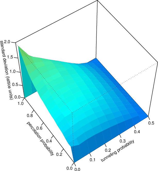
(d) for dynamic gaps.
The in figure 7(a) is as one would expect, with the gaps having a big impact on the spreading for low tunneling rates, while even a small amount of tunneling allows the spreading rate to steadily recover. The in figure 7(b) shows that this behaviour is reliable (low variation) except where both the number of gaps and the tunneling rate are low.
For dynamic gaps, the equivalent pair of plots are shown in figures 7(c) and 7(d). The introduction of dynamic gaps can be seen to have a steep but less drastic effect than static gaps by comparing figure 7(a) with figure 7(c). The is also lower, indicating the behaviour is less variable between different lattices with the same percolation probability . This is due to the dynamic gaps providing an averaging effect during the course of the walk.
The main message from these results for quantum walks on a line with edges missing is that a random pattern of missing edges leads to decoherence in the quantum walk, reducing the spreading to the classical random walk scaling proportional to , but with varying prefactors. However, the crossover to classical scaling happens quite slowly, after a crossover time proportional to as found by Romanelli et al. [32] for the case of dynamic gaps. This means the decoherence effects are minimal for smaller systems allowing the full quantum speed up to be exploited, while larger systems will only benefit from a prefactor enhancing the classical scaling.
3 Walk on a two-dimensional grid
A two-dimensional lattice allows a wider range of behaviour to be studied, without resorting to quantum tunneling. Since there is more than one path between two points on the lattice, the walker can take a (probably longer) path around the gaps when they are at a low density. Each vertex in a 2D lattice has four edges connected to it, so the quantum walker now needs a four-dimensional coin. We label the four directions , corresponding to and on the axis and , for and on the axis. The operator for “tossing” the coin can now be any unitary. The most common choice is based on Grover’s diffusion operator,
| (13) |
The general form of Grover’s diffusion operator for a -edged vertex is , it happens to be unbiased only for . It is chosen because of its symmetry, the incoming edge receives a sign flip, but the other three edges are treated equally. There are many possible unbiased coin operators based on generalised Hadamard matrices [44], but these will have other phases that treat the outgoing directions differently.
To complement this choice of coin operator, the shift operator must also invert the coin states,
| (14) |
This ensures that the coin operator is then applied to a coin state that labels the edge from which the walker arrived, which is the one that receives the minus sign from the Grover coin operator. For example,
| (15) |
First we recall the behaviour of a quantum walk on a lattice with all edges present. This is illustrated in figure 8.


For most choices of coin and initial state, the quantum walk tends to stay around the origin. For a well-behaved coin (with a good degree of symmetry), there is one precisely chosen state for which it spreads out in a ring of variable height that resembles a circular version of the walk on the line [34]. If we start the walker off from the origin (, ), we can use the average distance of the walker from the origin , the average of , as a measure of the spreading. This is playing the same role as for the walk on the line, although is more directly comparable with the average of , since the square root is taken before the averaging. In figure 8, the cases with the two extreme values of for the Grover coin operator are shown, on the left after 40 steps is 33.1, while on the right it is only 7.2. Nonetheless, this still represents a quantum spreading rate, despite the apparent dominance of the central peak. The classical spreading of is only 6.3 for 40 steps. Other initial states show a mixture of the ring and central peak, with corresponding intermediate spreading rates. However, the central peak is present and dominates over the ring for all except the symmetric starting state. This is in sharp contrast with the walk on the line where the spreading rate is the same for all initial coin states, only the symmetry of the distribution changes. Analytic treatment of the quantum walk in two dimensions has been provided by Grimmett et al. [45] and Gottlieb et al. [46].
3.1 Two-dimensional percolation lattices
Applying a quantum walk to a two-dimensional percolation lattice is a straightforward extension of the techniques already described for varying the dynamics of the walk on the line. For both bond and site percolation, the resulting lattice will in general contains vertices of degree 4, 3, 2, 1 and 0. Each needs an appropriate coin operator. We constructed these in the most symmetric possible way, basing the lower dimensional coins on the lower dimensional Grover operators padded with (minus) the identity for the directions where the edges are missing. For example, if the edge is missing, the coin operator becomes
| (16) |
while if both the and edges are missing,
| (17) |
Provided the initial state is correctly chosen, so the subspace of the missing edges is never populated, it doesn’t matter what appears in those rows and columns of the coin operators. However, if one wishes to interpolate between missing edges and the full lattice, in a generalisation of the tunnelling studied on the line in the previous section, the sign of the entries on the diagonal must be the same throughout the coin operator, as shown above. For consistency, the coin operator for all but one edge missing
| (18) |
applies a minus sign to the amplitude before it returns along the edge.
Since the initial coin state has a significant effect on the spreading rate of the walk, we therefore tested several different initial coin states, to see how this affected the behaviour, in combination with the missing edges in the percolation lattices. We tested the initial states and that give the maximum and minimum spreading rates as shown in figure 8,
| (19) |
and
| (20) |
These differ only in the phases between the different coin directions. We thus also tested random phases of between the different coin directions,
| (21) |
This is a similar strategy to that used by Tregenna et al. [34] when obtaining the maximum and minimum spreading rates. Restricting the variation to phases avoids skewing the walk, which would systematically increase the average distance traveled, making it harder to extract the generic average behaviour from the results. In all cases, the walker started at the origin. If there happened to be missing edges, those coin states were deleted from the initial state, and the remainder renormalized. If all the edges happened to be missing around the origin, a spreading of was recorded, since no walk was possible.
For each initial state in equations (19) to (21), we performed a numerical simulation of a quantum walk on both site and bond percolation lattices, averaging over 5000 randomly generated lattices of each type. We were able to run up to 140 time steps on a 3GHz processor in reasonable time (a week per 5000 sample lattices per initial state). With lattice sites, this is equivalent in memory requirements to nearly 40000 steps of a walk on a line. Arguably, 5000 sample lattices is not a sufficiently large sample for such large lattices. We investigated the sensitivity to sample size by comparing averages for smaller lattices (40 to 80 time steps) for 1000, 5000 and 20000 samples. The larger samples produced smoother averages as expected, but the smaller samples gave good enough results to draw conclusions from.
Figures 9, 10 and 11 present the results of these simulations in three complementary ways. In figure 9, we show the results for quantum walks with random phases in their initial states. The average distance from the starting position at the origin for a single quantum walk, where , is given by
| (22) |
Here is the probability of finding the particle at the site , i.e., summed over all coin states, and the sum over is over all lattice sites that could be reached by the walker, i.e., . Clearly, can vary, depending on the exact arrangement of missing sites or edges in the percolation lattice. We have therefore further averaged over 5000 random instances of bond or site percolation lattices, and plotted the resulting as a function of the percolation probability , for different lengths of quantum walk from 10 to 140 steps.

Values of below one that occur for small are not interesting: the low density of sites or edges in the lattice means that most of the time the quantum walk is unable to move from its starting state. While there is clearly some noise in the data, particularly for site percolation, the trends are clear. At around for bond ( for site) percolation, starts to rise. This is still below the critical probability () and the value of is not sensitive to the number of time steps because in general it is still confined to a small local region and cannot see the full size of the lattice. We then observe the lines for different time steps separating out below the main bundle in succession, smallest first, and flattening off towards the corresponding value for the complete lattice at . This is a nice illustration of finite size effects. The size of the localized clusters grows as approaches from below. As the cluster size becomes comparable with the size of the walk (10, 20 time steps, etc.), the limitation of due to cluster size is replaced by limitation due to the number of steps, and the walk is no longer sensitive to increasing cluster size. Walks of about 100 steps or longer are still close to synchronized at , indicating that quantum walks of this size should provide good estimates of critical parameters.
In the region where , the rate of growth of slows then steepens again. For , the walk no longer distinguishes between bond and site percolation, is the same for both. This is somewhat surprising, because removing a site from the lattice removes four neighbouring edges, compared to removing a single edge for bond percolation. It suggests that in the regime where missing sites or edges can be expected to be isolated from each other, they both behave as lattice defects, with the broken lattice symmetry more important that the detailed structure of the defect.
To understand this behaviour in more detail, we turn to figure 10, where walks of 60 time steps are compared for all three initial states.


Also plotted is , the standard deviation of , to quantify how variable the spreading is between different percolation lattices. Note first that the average spreading for ranges from around 14 for to 35 for . The value for is around 18, half that for . However, for is around seven, indicating that the average value conceals significant variation over the random phases. This is as expected, since the randomly chosen phases should include both and . The position of close to indicates the weight of the distribution lies nearer the minimum spreading rather than the maximum. All this is already known from previous studies, of course, but it is useful to recall the details before considering the behaviour for .
Looking at the standard deviations, it can be seen that the variation for is larger for site percolation, typically around five compared with around two for bond percolation for . Thus, although the average behaviour is similar, missing sites produce more extreme cases (high and low) for the same number of missing bonds in bond percolation. This suggests further work to elucidate the source of this difference would be fruitful.
The variation of over time with can be plotted in 3D, see figure 11 for two examples.


This shows how similar the behaviour is for both bond and site percolation, with any choice of initial state, but it does not bring out the most interesting features to do with how the scaling varies with the percolation probability. The necessary scaling analysis is described in the following subsection.
3.2 Scaling analysis

Apart from a regular zigzag over a cycle of four steps, due to the lattice and coin symmetries, the line for a fixed value of is very close to a straight line, with slope varying from zero (small ) to one (). This suggests the data will be well fit by with . Mindful of the finite size effects discussed in relation to figure 9, fits to determine were done using only the data for time steps 100 to 140. The resulting values for the exponent are shown in figure 13.

The values of agree fairly well with the expectation that the first rise above zero should be seen around the critical point (bond) and (site). The initial state that produces maximum spreading has a noticeably higher exponent, around 0.05 larger than for random phases or the minimum spreading state, from the critical point through to near , implying that the advantage of the optimal initial state is not just a prefactor on the same scaling rate. All initial states follow the same overall pattern of a steady rise from the critical point, a flattening off towards , the classical exponent for the perfect lattice, in the region of , followed by a steep rise to the quantum spreading rate of .
To test the influence of finite size effects on these results, the same fits were done using more of the data, with and as lower cut off points in place of . The slightly higher exponents these fits produce are shown as an inset in figure 13, along with more detailed data, for the case with random phase initial states. These show that the trend towards lower values of is slow, and hence, based on these simulations, we cannot make a strong prediction for what the asymptotic variation of the exponent with percolation rate is going to be. Nonetheless, we can confidently say that for systems of limited size, there is a significant window for in which the quantum advantage exists in the form of faster spreading than a classical random walk.
4 Summary and discussion
Even for the simple case of a coined quantum walk on the line we find contrasting effects brought about by the interplay between missing edges and quantum tunnelling, in the presence of ordered or disordered arrangements of the missing edges. Ultimately, for long times, the disorder of random missing edges causes the spreading to reduce to the classical rate. Yet for shorter walks, even up to a thousand steps, the spreading is still largely dominated by quantum effects. And for ordered arrangements of missing edges, the quantum spreading rate is maintained, though with varying prefactors. These results are consistent with those of a number of other analytical and numerical studies, in particular Romanelli et al. [32] who first studied randomly changing gaps on the line, and Linden and Sharam [42], who provide detailed analytic treatment of periodically varying coins. The connections between disorder and decoherence were discussed in detail by Romanelli et al., highlighting the role of randomness from whatever source in degrading the quantum coherence. The scaling of quantum walks on the line with decoherence or other sources of disorder are in general either linear spreading or spreading, with different prefactors depending on the details of the dynamics. Intermediate scaling in one-dimensional walks is not obtained except transiently as linear crosses over to a long time limit of .
In contrast to the 1D cases, on 2D percolation lattices we find the quantum walks show fractional scaling of the spreading, i.e., for , with . Classical random walks on percolation lattices also exhibit fractional scaling behaviour, with . One interesting question is whether this behaviour seen for finite-sized walks extends to the long time limit. Although our simulations seem to have reached a size where finite size effects are small, the slow convergence, coupled with the lessons from one dimensional quantum walks where decoherence dominated only after thousands of steps, means we do not think we can confidently predict the large behaviour. For example, a possibility consistent with our results is that the steep rise in the region of will becomes a “step” function at as , and that the portion below will follow the scaling for classical random walks. The intuition for this is that the randomness in the percolation lattice would thus again act as decoherence in the large limit. Whether this is correct depends on whether a very small density of defects is enough to disrupt the entire walk in the whole two-dimensional lattice in the long time limit. Studies of absorbing boundaries and trapping are relevant to this question, in one dimension the presence of traps does not inevitably catch a quantum walker [33], while a classical walker will eventually fall into a single trap in both one and two dimensions. This will be an interesting question to answer because trapping behaviour is particularly important for models of exciton transport, as discussed by Mülken et al. [47], and trapping can also be exploited to guide the exciton to the desired location. Feldman and Hillery [48] and Hillery et al. [49] provide a scattering matrix method for treating finite graphs analytically, and determining solutions that traverse the graph or are trapped within it. This may provide a route to understanding how structures in the percolation lattice contribute to trapping the quantum walker.

Aside from the question of trapping behaviour, we offer some further intriguing observations that suggest directions for future study. Figure 14 shows the data for random initial states from figure 13 plotted along with numerical results for running a classical random walk on percolation lattices up to 140 steps, and processed to extract the scaling in exactly the same way. The first and most obvious problem is that 140 steps of a classical random walk still suffers from large finite size effects! This is easily understood, for a classical random walk on the fully connected lattice is , which is about 12 for . This is more comparable with for a quantum walk (with random phases in the initial state), as can be obtained from figure 9, reading off the values for . Since gives an indication of the size of the largest structures that the quantum or random walk will be sensitive to, if the missing sites or edges are on average further apart than that, the walker will hardly notice any before finishing the walk and reporting its position. Working in the other direction, a quantum walk of 100 steps (with random phase initial state) has . If we want a classical random walk with , will need to run it for steps! The advantage of the linear scaling with of the quantum walks is suddenly very apparent.
As already noted, we appear to have achieved a reasonable convergence of finite size effects on percolation lattices by running a classical simulation of a quantum walk for 100 or more steps. These simulations required around a week of processor time on a fast workstation, a fairly modest amount of computational resources. This suggests that using such simulations to obtain numerical values for percolation lattice parameters is worth investigating. In other words, this could provide a route to improved classical simulation methods. There are other examples of quantum algorithms providing better classical methods, Love and Boghosian [50] discuss a number of examples in detail.
However, the main reason for running the classical random walk was to compare with the quantum walk and further understand our results. Much larger classical simulations were not possible with our available computational resources, we would have needed an order of magnitude more computational power, or to implement more efficient simulation techniques. Comparisons using the results in figure 14 can only be suggestive, nonetheless, the suggestions are intriguing. If we assume that the shape of the classical curves in figure 14 won’t change much, so they will simply shift to the right as finite size effects reduce, then we can compare the shape with the curves for quantum walks. For site percolation, the classical and quantum curves are the same shape up to about on the quantum curve. The corresponding curves for bond percolation are not, however, the quantum curve lies significantly below the classical curve for the region . This adds further evidence for basic differences in quantum walk behaviour on bond and site percolation lattices that the differences in standard deviation noted in figure 10 imply. In particular, that quantum walks are slower than classical in some regions, while faster than classical in others. Such behaviour has been noted in other contexts, see for example Agliari et al. [51].
Nonetheless, the main message we want to emphasize from this study is that for modest system sizes of a few hundred sites, and defect densities below 10%, faster-than-classical fractional scaling is very much the dominant feature. This is an interesting regime with many applications in both bio- and nano-scale materials, where quantum effects are important to fully understand their properties and behaviour.
Acknowledgments
We thank Jiajun Tan for assistance in preparing the references for this paper. VK is funded by a Royal Society University Research Fellowship. PK was funded by a Nuffield Undergraduate Summer Bursary. JB was funded by a Royal Society Summer Bursary. GLMC was funded by the University of Leeds School of Physics and Astronomy Summer Bursary scheme.
References
- [1] E Farhi and S Gutmann. Quantum computation and decison trees. Phys. Rev. A, 58:915–928, 1998.
- [2] Aharonov, D, A Ambainis, J Kempe, and U Vazirani. Quantum walks on graphs. In Proc. 33rd Annual ACM STOC, pages 50–59. ACM, NY, 2001.
- [3] Andris Ambainis, Eric Bach, Ashwin Nayak, Ashvin Vishwanath, and John Watrous. One-dimensional quantum walks. In Proc. 33rd Annual ACM STOC, pages 60–69. ACM, NY, 2001.
- [4] Julia Kempe. Quantum random walks hit exponentially faster. In Proc. 7th Intl. Workshop on Randomization and Approximation Techniques in Computer Science (RANDOM ’03), Lecture Notes in Computer Science, pages 354–369. Springer, Heidelberg, 2003.
- [5] Julia Kempe. Quantum random walks hit exponentially faster. Probability Th. and Related Fields, 133(2):215–235, 2005.
- [6] Andrew M. Childs, Richard Cleve, Enrico Deotto, Edward Farhi, Sam Gutmann, and Daniel A. Spielman. Exponential algorithmic speedup by a quantum walk. In Proc. 35th Annual ACM STOC, pages 59–68. ACM, NY, 2003. ArXiv:quant-ph/0209131.
- [7] J P Keating, N Linden, J C F Matthews, and A Winter. Localization and its consequences for quantum walk algorithms and quantum communication. Phys. Rev. A, 76:012315, 2007. ArXiv: quant-ph/0606205.
- [8] Hari Krovi and Todd A. Brun. Hitting time for quantum walks on the hypercube. Phys. Rev. A, 73(3):032341, 2006a.
- [9] Hari Krovi and Todd A. Brun. Quantum walks with infinite hitting times. Phys. Rev. A, 74(4):042334, 2006b.
- [10] Hari Krovi and Todd A. Brun. Quantum walks on quotient graphs. Phys. Rev. A, 75:062332, 2007.
- [11] M. Štefaňák, I. Jex, and T. Kiss. Recurrence and pólya number of quantum walks. Phys. Rev. Lett., 100(2):020501, Jan 2008a. doi: 10.1103/PhysRevLett.100.020501.
- [12] M. Štefaňák, T. Kiss, and I. Jex. Recurrence properties of unbiased coined quantum walks on infinite -dimensional lattices. Phys. Rev. A, 78(3):032306, Sep 2008b. doi: 10.1103/PhysRevA.78.032306.
- [13] Neil Shenvi, Julia Kempe, and K Birgitta Whaley. A quantum random walk search algorithm. Phys. Rev. A, 67:052307, 2003. ArXiv:quant-ph/0210064.
- [14] Charles H Bennett, Ethan Bernstein, Gilles Brassard, and Umesh Vazirani. Strengths and weaknesses of quantum computing. SIAM J. Comput., 26(5):151–152, 1997.
- [15] Miklos Santha. Quantum walk based search algorithms. In 5th Theory and Applications of Models of Computation (TAMC08), Xian, April 2008, volume 4978, pages 31–46. LNCS, 2008.
- [16] S. Bose. Quantum communication through an unmodulated spin chain. Phys. Rev. Lett., 91(20):207901, 2003.
- [17] M. Mohseni, P. Rebentrost, S. Lloyd, and A. Aspuru-Guzik. Environment-assisted quantum walks in photosynthetic energy transfer. J. Chem. Phys., 129:174106, 2008.
- [18] Vivien M. Kendon and Christino Tamon. Perfect state transfer in quantum walks on graphs. J. Comp. Theor. Nanoscience, 2010. Invited contribution, to appear in special issue on “Novel Biochemical and Physical Information Processing Systems”, ed. Dmitry Solenov and Vladimir Privman.
- [19] Elena Agliari, Oliver Muelken, and Alexander Blumen. Continuous-time quantum walks and trapping. International Journal of Bifurcation and Chaos, 2009. To appear, arXiv.org:0903.3288v2.
- [20] H Eugene Stanley Zorica V Djordjevic and Alla Margolina. Site percolation threshold for honeycomb and square lattices. J. Phys. A: Math. Gen., 15:L405–L412, 1982.
- [21] T. Gebele. Site percolation threshold for square lattice. J. Phys. A: Math. Gen., 17:L51–L54, 1984.
- [22] Dietrich Stauffer and Ammon Aharony. Introduction To Percolation Theory. CRC, July 1994. ISBN 0748402535.
- [23] X.P. Xu and F. Liu. Continuous-time quantum walks on Erdös-Rényi networks. Physics Letters A, 372(45):6727–6732, 2008. ISSN 0375-9601. doi: DOI: 10.1016/j.physleta.2008.09.042.
- [24] Aharonov, Y, L Davidovich, and N Zagury. Quantum random walks. Phys. Rev. A, 48(2):1687–1690, 1992.
- [25] J Watrous. Quantum simulations of classical random walks and undirected graph connectivity. J. Comp. System Sciences, 62(2):376–391, 2001.
- [26] A. Romanelli, A. C. Sicardi-Schifino, R. Siri, G. Abal, A. Auyuanet, and R. Donangelo. Quantum random walk on the line as a Markovian process. Physica A, 338:395–405, 2004.
- [27] A Nayak and A Vishwanath. Quantum walk on the line. Extended abstract, ArXiv: quant-ph/0010117, 2000.
- [28] Hilary A Carteret, Mouraid A Ismail, and Bruce Richmond. Three routes to the exact asymptotics for the one-dimensional quantum walk. J. Phys. A, 36(33):8775–8795, 2003.
- [29] Norio Konno, Takao Namiki, and Takahiro Soshi. Symmetricity of distribution for the one-dimentional Hadamard walk. Interdisciplinary Infor. Sci., 10(1):11–22, 2004.
- [30] Norio Konno. A new type of limit theorems for the one-dimensional quantum random walk. Journal of the Mathematical Society of Japan, 57(4):1179–1195, 2005a.
- [31] Peter L Knight, Eugenio Roldán, and J E Sipe. Propagating quantum walks: the origin of interference structures. J. Mod. Opt., 51:1761–1777, 2004.
- [32] A. Romanelli, R. Siri, G. Abal, A. Auyuanet, and R. Donangelo. Decoherence in the quantum walk on the line. Physica A, 347:137–152, 2003.
- [33] Eric Bach, Susan Coppersmith, Marcel Paz Goldschen, Robert Joynt, and John Watrous. One-dimensional quantum walks with absorbing boundaries. J. Comput. Syst. Sci., 69(4):562–592, 2004.
- [34] Ben Tregenna, Will Flanagan, Rik Maile, and Viv Kendon. Controlling discrete quantum walks: coins and initial states. New J. Phys., 5:83, 2003.
- [35] Norrio Konno. A path integral approach for disordered quantum walks in one dimension. Fluctuation and Noise Letters, 5(4):529–537, 2005b.
- [36] Viv Kendon. Decoherence in quantum walks – a review. Math. Struct. in Comp. Sci., 17(6):1169–1220, 2007. ArXiv: quant-ph/0606016.
- [37] Steve Park and Keith Miller. Random number generators: Good ones are hard to find. Communications of the ACM, 31:1192–1201, 1998.
- [38] Todd A Brun, H A Carteret, and Andris Ambainis. Quantum random walks with decoherent coins. Phys. Rev. A, 67:032304, 2003a.
- [39] Todd A Brun, H A Carteret, and Andris Ambainis. The quantum to classical transition for random walks. Phys. Rev. Lett., 91(13):130602, 2003b.
- [40] W Dür, R Raussendorf, V M Kendon, and H-J Briegel. Quantum random walks in optical lattices. Phys. Rev. A, 66:052319, 2002.
- [41] Mostafa Annabestani, Seyed Javad Akhtarshenas, and Mohamed Reza Abolhassani. Tunneling effects in a one-dimentional quantum walk, 2010. arXiv:1004.4352v1.
- [42] Noah Linden and James Sharam. Inhomogeneous quantum walks. Phys. Rev. A, 80(5):052327, Nov 2009. doi: 10.1103/PhysRevA.80.052327. arXiv:0906.3692v1.
- [43] Yutaka Shikano and Hosho Katsura. Localization and fractality in inhomogeneous quantum walks with self-duality, 2010. arXiv:1004.5394v1.
- [44] Życzkowski K. Tadej W. A concise guide to complex hadamard matrices. Open Systems & Infor. Dyn., 13:133–177, 2006.
- [45] Geoffrey Grimmett, Svante Janson, and Petra Scudo. Weak limits for quantum random walks. Phys. Rev. E, 69:026119, 2004.
- [46] Alex D Gottlieb, Svente Janson, and Petra F Scudo. Convergence of coined quantum walks in . Inf. Dimen. Anal. Quantum Probab. Rel. Topics, 8(1):129–140, 2005.
- [47] Oliver Mülken, Alexander Blumen, Thomas Amthor, Christian Giese, Markus Reetz-Lamour, and Matthias Weidemüller. Survival probabilities in coherent exciton transfer with trapping. Phys. Rev. Lett., 99(9):090601, Aug 2007. doi: 10.1103/PhysRevLett.99.090601.
- [48] Edgar Feldman and Mark Hillery. Scattering theory and discrete-time quantum walks. Phys. Lett. A, 324(3):277, 2004.
- [49] Mark Hillery, Janos Bergou, and Edgar Feldman. Quantum walks based on an interferometric analogy. Phys. Rev. A, 68(3):032314, 2003.
- [50] Peter J. Love and Bruce M. Boghosian. Type II quantum algorithms. Physica A: Statistical Mechanics and its Applications, 362(1):210–214, 2006. ISSN 0378-4371. doi: DOI: 10.1016/j.physa.2005.09.017. Discrete Simulation of Fluid Dynamics - Proceedings of the 13th International Conference on Discrete Simulation of Fluid Dynamics.
- [51] E Agliari, A Blumen, and O Mülken. Dynamics of continuous-time quantum walks in restricted geometries. Journal of Physics A: Mathematical and Theoretical, 41(44):445301, 2008.