Body-and-cad geometric constraint systems
Abstract
Motivated by constraint-based CAD software, we develop the foundation for the rigidity theory of a very general model: the body-and-cad structure, composed of rigid bodies in 3D constrained by pairwise coincidence, angular and distance constraints. We identify 21 relevant geometric constraints and develop the corresponding infinitesimal rigidity theory for these structures. The classical body-and-bar rigidity model can be viewed as a body-and-cad structure that uses only one constraint from this new class.
As a consequence, we identify a new, necessary, but not sufficient, counting condition for minimal rigidity of body-and-cad structures: nested sparsity. This is a slight generalization of the well-known sparsity condition of Maxwell.
1 Introduction
This paper initiates the study of and sets up the foundation for the rigidity theory of a large class of 3D geometric constraint systems. These systems are composed of rigid bodies with specific coincidence, angular and distance constraints and are called body-and-cad structures. To the best of our knowledge, these constraints have not been systematically studied before from this perspective.
Motivation. Popular computer aided design (CAD) software applications based on geometric constraint solvers allow users to design complex 3D systems by placing geometric constraints among sets of rigid body building blocks. The constraints are specified by identifying geometric elements (points, lines, planes, or splines) on participating rigid bodies. Detecting when a user has created a fully-defined sub-system or has added a redundant (or inconsistent) constraint are important problems for providing informative feedback. However, analyzing all constraints simultaneously is a very difficult problem. In this paper, we focus on a subset of these constraints that are amenable to a rigidity-theoretical investigation.
Underlying classical rigidity theory results is a general proof pattern, spanning algebraic geometry (for rigidity), linear algebra (for infinitesimal rigidity) and graph theory (for combinatorial rigidity). The ultimate goal is a full combinatorial characterization of generically minimally rigid structures, but such results are extremely rare: 3D bar-and-joint rigidity remains a conspicuously open problem [7], while the 2D version is fully understood [12]. An important step along the way is identifying a pattern in the rigidity matrix developed as part of the infinitesimal rigidity theory for the structures. While this is straightforward for the well-known bar-and-joint model, it is more complicated in the body-and-bar model. In this paper, we formulate the even more involved rigidity matrix for the body-and-cad model.
Results. We define a body-and-cad structure to be composed of rigid bodies connected by pairwise coincidence, angular (parallel, perpendicular, or arbitrary fixed angular) and distance constraints. The constraints occur between specified points, lines or planes (called geometric elements). Besides the well-studied distance constraint between points (as in body-and-bar structures), we identify 20 new pairwise constraints. We label constraints by the geometric elements involved, e.g., a line-plane perpendicular constraint between bodies and indicates that a line on is perpendicular to a plane on . The complete set of body-and-cad constraints that we study is further subdivided into six categories:
- •
Point-point constraints: coincidence, distance.
- •
Point-line constraints: coincidence, distance.
- •
Point-plane constraints: coincidence, distance.
- •
Line-line constraints: parallel, perpendicular, fixed angular, coincidence, distance.
- •
Line-plane constraints: parallel, perpendicular, fixed angular, coincidence, distance.
- •
Plane-plane constraints: parallel, perpendicular, fixed angular, coincidence, distance.
We develop the pattern of the rigidity matrix and identify a necessary combinatorial counting property called nested sparsity, which is the counterpart of the well-known Maxwell condition [18] for fixed length rigidity. We also show that this condition is not sufficient. However, it can be used as a filter for finding candidate rigid components. Finally, we present an efficient algorithm for nested sparsity, based on pebble game algorithms previously developed for sparse graphs.
Related work. Classical rigidity theory [7] focuses on distance constraints between points [12] or rigid bodies [30, 34]. Direction constraints (where 2 points are required to define a fixed direction, with respect to a global coordinate system) are well-understood and arise from parallel redrawing applications [35]. Motivated by CAD systems, Servatius and Whiteley present a characterization, which can be viewed as a generalized Laman counting property, for 2D systems with both length and direction constraints [24].
Work on angular constraints has also focused on combinatorial characterization results. Zhou and Sitharam [37] characterize a large class of 2D angular constraint systems along with a set of combinatorial construction rules that maintain generic independence. Saliola and Whiteley [21] prove that, even in the plane, the complexity of determining the independence of a set of circle intersection angles is the same as that of generic bar-and-joint rigidity in 3D. A full characterization for angular constraints of the nature that appear in this paper is further described in [16, 13].
Combinatorial sparsity conditions are intimately tied with rigidity theory, appearing often as necessary conditions (as for bar-and-joint rigidity) and sometimes even as complete characterizations (as for 2D bar-and-joint and body-and-bar frameworks in arbitrary dimension) [36, 12, 30]. Pebble game algorithms have been developed for solving sparsity problems [14, 29, 15]. These algorithms do not apply, however, to the so-called -counting conditions known to be a necessary, but not sufficient, condition for 3D bar-and-joint rigidity. In fact, no efficient algorithm is known for these counts.
Related work on the constraints studied in this paper has appeared in the CAD research community, usually within the context of decomposition approaches; a survey may be found in [25, 11]. In this setting, a geometric constraint system (GCS) is formulated as an algebraic system of equations. Due to the complexity of solving such a system, it is traditionally decomposed into structured sub-systems that can be solved and later recombined to obtain a solution to the original GCS. In the process of decomposition, approximate notions of combinatorial rigidity have been used [10, 9].
Results in the CAD literature have observed that angular constraints exhibit special behavior. For the so-called generalized Stewart platform, [5] gives explicit equations that highlight this distinction. Gao et al. [6] present a method for analyzing 2D and 3D systems with a restricted set of coincidence, angular and distance constraints. Both [5] and [6] treat angular constraints separately, implicitly using natural necessary counting conditions to do so. We consider analogous systems from the rigidity theory perspective, expressing them infinitesimally using Grassmann-Cayley algebra; the shape of the rigidity matrix described in Section 3 explicitly reveals the distinct treatment of angular constraints. Grassmann-Cayley, Clifford algebras and geometric algebras often appears in the context of CAD or geometric theorem proving; see, e.g., [17, 23]. Recent work of [20] expresses constraints from a similar perspective when providing a foundation for software to build a GCS.
Incidence constraints have been studied previously in connection with Geometric Theorem Proving [17, 19] for projective incidence theorems. Sitharam et al. [26, 27, 28] formalize the question of obtaining a well-formed and optimal system of algebraic equations to resolve a collection of incident rigid bodies. [26] studies “well-formedness,” a condition necessary to avoid dependent equations, and a new, underlying matroid whose independent sets capture this. A combinatorial measure of algebraic complexity of the system of equations is described in [27], and another underlying matroid is used to optimize this measure. In [28], it is shown how to reconcile the independent sets of the prvious two matroids to obtain an optimal, well-formed system.
Structure. Section 2 gives a brief overview of the required mathematical background. Section 3 develops the foundations for the infinitesimal rigidity theory, providing the basic building blocks used for each new constraint. Each of the full set of constraints is then expressed using these building blocks in Section 4, resulting in the complete derivation of the rigidity matrix. Section 5 identifies a new combinatorial property resulting from the structure of the rigidity matrix; this nested sparsity condition, while necessary, is shown not to be sufficient with a counterexample. Section 6 presents algorithms for nested sparsity using pebble games as oracles. Finally, Section 7 discusses extensions, applications and future directions.
2 Preliminaries
Our results rely on the same mathematical background as the work on body-and-bar rigidity by Tay [30] and White and Whiteley [34]. We use Grassmann-Cayley algebra, Plücker coordinates and instantaneous screw theory (see, e.g., [32, 33] and [22]). For self-containment, we briefly introduce notation and basic concepts from the Grassmann-Cayley algebra and its correspondence with instantaneous screws.
2.1 Terminology and notation.
We restrict ourselves to dimension 3 in this paper; 2-tensors in the Grassmann-Cayley algebra (see, e.g., [32, 33]) are identified with vectors in . The Grassmann-Cayley join operator is represented with . The join of two vectors is the collection of all 6 minors of the matrix obtained with and as its rows. We fix a convention at this point to order the minors in a 6-vector as 11 1 We remark that other papers (e.g., [30] and [34]), use a different convention by fixing the order as . The dot product of two vectors and is denoted . The star operator ∗ swaps the first and last 3 coordinates of a 6-vector. If and , we denote by the vector of length 4 obtained by appending to .
Rigid body motions. The theory of screws was introduced by Ball [1] as a way of expressing rigid body motion. Rigid body transformations are associated with elements of the special Euclidean group . By Chasles’ Theorem from 1830 (see [22]), they can also be expressed as screw motions (see Figure 1a). It follows that every instantaneous rigid body motion can be expressed as an instantaneous screw motion (see Figure 1b); for further details, we refer the reader to a standard text, e.g., page 24 of [22].


Both screw motions and instantaneous screw motions are defined with respect to a screw axis along with a rotation about the axis and a translation along it.
In this paper, we are concerned only with instantaneous screw motions, which, for brevity, will be referred to as instantaneous screws. An instantaneous screw is represented by a 6-vector , where ; the minus sign in front of is a convenient, technical convention. The first component encodes the angular velocity; as a vector, gives the direction of the screw axis, and its magnitude encodes the angular speed. The translational velocity can be computed from and , but we skip the details as they are not relevant for the rest of the paper. Note that the star operator applied to a screw gives . There is an exact correspondence between 2-tensors and instantaneous screws. This correspondence is the key to describing the rigidity matrix of the body-and-cad structures.
2.2 Body-and-cad structures
A body-and-cad structure in 3D is composed of bodies interconnected by pairwise constraints. Each body is represented by a frame of reference, specified by a transformation matrix from the special Euclidean group . Each body additionally has a set of geometric elements (points, lines or planes) identified as attachments for the constraints.
Representation of geometric elements. Each geometric element is rigidly affixed to a body and is described with coordinates that are local with respect to the frame of reference for body . For ease of analysis, we represent a plane in point-normal form as the pair , with , where is a point on the plane and is the normal to the plane. We represent a line in parametric form, given by the pair , with , where is a point on the line and is its direction.
2.2.1 Cad graphs
We now introduce the cad graph, our main combinatorial object for body-and-cad rigidity.
To illustrate this concept, consider the following example, depicted in Figure 2. Let and be two dice rigidly stacked with the following constraints: (i) (plane-plane parallel) ’s Face 1 is parallel to ’s Face 1, (ii) (plane-plane perpendicular) ’s Face 2 is perpendicular to ’s Face 3, (iii) (line-plane distance) The distance between ’s Line 12 (intersection of Faces 1 and 2) and ’s Face 1 is 1, and (iv) (point-point coincidence) ’s Corner 236 (the point defined by Faces 2, 3 and 6) is coincident to ’s Corner 123.

These constraints are captured by a graph with two nodes connected by annotated edges called the cad graph; see Figure 3.
Formally, a cad graph is a multigraph together with an edge coloring function , where consists of 21 colors corresponding to the full set of cad constraints:
- 1.
point-point coincidence
- 2.
point-point distance
- 3.
point-line coincidence
- 4.
point-line distance
- 5.
point-plane coincidence
- 6.
point-plane distance
- 7.
line-line parallel
- 8.
line-line perpendicular
- 9.
line-line fixed angular
- 10.
line-line coincidence
- 11.
line-line distance
- 12.
line-plane parallel
- 13.
line-plane perpendicular
- 14.
line-plane fixed angular
- 15.
line-plane coincidence
- 16.
line-plane distance
- 17.
plane-plane parallel
- 18.
plane-plane perpendicular
- 19.
plane-plane fixed angular
- 20.
plane-plane coincidence
- 21.
plane-plane distance
The geometric meaning of these colors will be described in the next section; the cad graph only captures the type of constraint imposed.
2.2.2 Body-and-cad frameworks
A body-and-cad framework is a cad graph along with a family of functions describing the geometry of the structure, where the function captures the constraints corresponding to edges with the th color. Let be the set of -colored edges.
For example, the function for plane-plane fixed angular constraints maps an edge to a triple so that the planes and affixed to bodies , respectively , are constrained to have the angle between them. The function for point-point coincidence constraints maps an edge to a pair of points affixed to bodies , respectively , that are constrained to be coincident. We will define the complete family of functions when analyzing them individually in Section 4.
A realization of a body-and-cad framework assigns a tuple of frames for each vertex, satisfying the specified constraints. In this paper, we are not concerned with realization questions. We will always assume that a body-and-cad framework is given by a concrete realization, from which the family of functions is computed.
Body-and-cad rigidity. Intuitively, a body-and-cad framework is rigid if the only motions respecting the constraints are the trivial 3D motions (rotations and translations); otherwise, it is flexible. We omit the technical definition, as it falls outside the scope of this paper.
Body-and-cad minimal rigidity. For classical distance constraints, the concept of minimal rigidity is defined as follows: a structure is minimally rigid if the removal of any constraint results in a flexible structure. However, in our case, geometric constraints may correspond to more than one “primitive” constraint. Intuitively, a primitive constraint yields only one row in the rigidity matrix (formally defined in Section 3), while the body-and-cad constraints may yield several rows. In our setting, we define minimal rigidity as above, but referring to the removal of primitive constraints only: a rigid body-and-cad structure is minimally rigid if the removal of any primitive constraint results in a flexible structure.
We return to the example from Figure 2 to illustrate the subtleties of this concept. The structure depicted is rigid. We say the structure is overconstrained since it remains rigid even after the removal of constraint (iii). The resulting structure is now minimally rigid. As we will see in Section 3, constraints (i), (ii) and (iv) correspond to 6 primitive constraints. Thus, the removal of any primitive constraint results in a flexible structure.
Now consider stacking the dice with the following two constraints: (i) (line-line coincidence) ’s Line 26 is coincident to ’s Line 12 and (ii) (line-line coincidence) ’s Line 36 is coincident to ’s Line 13. This structure is still rigid. While it becomes flexible after the removal of either constraint (i) or (ii), it is not minimally rigid. As we will see in Section 3, a line-line coincidence constraint corresponds to 4 primitive constraints. Thus, this structure has 8 primitive constraints and is overconstrained. To give some intuition, note that a structure composed of 2 rigid bodies has 12 degrees of freedom. Of these, 6 are trivial, so we may fix body to factor them out. Now consider constraint (i); the structure is left with 2 degrees of freedom, as may slide along the line and rotate about it. This line-line coincidence constraint is “eliminating” 4 degrees of freedom, formalized by the 4 rows of the rigidity matrix developed in Section 3 for the line-line coincidence constraint.
Body-and-cad infinitesimal rigidity. Infinitesimal rigidity is the linearized version of rigidity and is the only type we study in this paper. Let assign an instantaneous screw to each body and let . The vector is an infinitesimal motion of a body-and-cad structure if it infinitesimally respects the constraints. This can be expressed with the help of the rigidity matrix, fully described in Section 3. An infinitesimal motion is a vector in the kernel of the rigidity matrix. The kernel always contains the trivial infinitesimal motions, defined as those with for all and .
A body-and-cad framework is infinitesimally rigid if the only infinitesimal motions are trivial; otherwise, it is infinitesimally flexible.
Remarks. To develop the rigidity theory for a new model, three steps must be accomplished.
- 1.
Algebraic theory. Formulate the rigidity concept in algebraic terms, resulting in an algebraic variety.
- 2.
Infinitesimal theory. Analyze the local behavior at some point on the algebraic variety. This reduces to the study of a rigidity matrix.
- 3.
Combinatorial rigidity. Seek a combinatorial characterization of minimal rigidity in terms of properties of an underlying graph structure. This is usually derived from properties of the rigidity matrix at a generic point on the algebraic variety.
In this paper, we directly formulate the infinitesimal rigidity theory for body-and-cad structures and identify combinatorial properties for the generic case.
To summarize, a cad graph is an edge-colored multigraph that captures the body-and-cad combinatorics, and a body-and-cad framework captures the geometry of the structure. As we develop the analysis of these concepts, an additional combinatorial object called the primitive cad graph will be associated to the cad graph. This is a multigraph with red or black edges, which captures certain combinatorial properties of infinitesimal body-and-cad rigidity.
3 Foundations of infinitesimal theory
The example from the previous section exposes some of the subtleties encountered with body-and-cad constraints that are not found when considering classical distance constraints. We introduce two new concepts to simplify the analysis: primitive angular and blind constraints. We then define, as building blocks, 4 basic angular and blind constraints and develop their infinitesimal theory. All 21 body-and-cad constraints can be studied using these building blocks, leading to the body-and-cad rigidity matrix.
3.1 Primitive constraints
A primitive constraint is one that may restrict at most one degree of freedom. For example, a point-point distance (bar) constraint is a primitive constraint, while the line-line coincidence constraint from the example in the preceding section is not. We classify primitive constraints into two types: angular and blind; as the theory is developed, it will become more clear why these classifications are appropriate, as they correspond to constraints demonstrating different algebraic behaviors.
A rigid body in 3D has 6 degrees of freedom, 3 of which are rotational and 3 of which are translational. A primitive angular constraint may restrict only a rotational degree of freedom, whereas a primitive blind constraint may restrict either a rotational or a translational degree of freedom. For instance, a line-line perpendicular constraint is a primitive angular constraint as it may restrict at most one rotational degree of freedom. A point-point distance (bar) constraint is a primitive blind constraint as it may restrict at most one rotational or translational degree of freedom. We will associate a set of primitive angular and a set of primitive blind constraints with each body-and-cad constraint.
3.2 Rigidity matrix
The rigidity matrix for a body-and-cad structure has 6 columns for each body , corresponding to the components of the instantaneous screw , as was done for the original body-and-bar rigidity matrix22 2 The starred version (see Section 2.1) will be used to conveniently order the columns of the rigidity matrix.. There is a row for each primitive constraint associated to the original body-and-cad structure. A primitive angular constraint results in a row containing zero entries in the first 3 columns for each body, while a primitive blind constraint may have non-zero entries in any of the 6 columns for each body. In the schematic below, gray cells indicate potentially non-zero entries, and red cells highlight the zero entries for angular constraints.
Since the trivial motions corresponding to the 3D rigid motions are necessarily in the kernel of , the maximum rank of is . By definition, a structure is infinitesimally rigid if its rigidity matrix has rank exactly .
| - | - | - | ||||||
| Angular | ||||||||
| constraints | ||||||||
| Blind | ||||||||
| constraints | ||||||||
3.3 Building blocks
We now define 4 very specific basic angular and blind constraints (2 of each) and develop the infinitesimal theory for them. Everything in Section 4 is derived from these basic building blocks. The material presented here is the most technical part of our paper.
Angular building blocks
All body-and-cad angular constraints can be
reduced to the following basic constraints
between pairs of lines:
(i) basic line-line non-parallel fixed angular, and
(ii) basic line-line parallel.
(i) Basic line-line non-parallel fixed angular. A line-line non-parallel angular constraint between bodies and is defined by identifying a pair of non-parallel lines, each rigidly affixed to one body, and fixing the angle between them. Let and be the directions of the lines affixed to bodies and , respectively. Then the constraint is infinitesimally maintained if the axis of the relative screw is in a direction lying in the plane determined by and , i.e.,
Since is composed of the last three coordinates of , this is equivalent to
| (3.1) |
This corresponds to one row in the rigidity matrix:
(ii) Basic line-line parallel constraint. A line-line parallel constraint between bodies and is defined by identifying a pair of parallel lines, each rigidly affixed to one body, and restricting them to remain parallel. Let be the direction of the parallel lines. Then the constraint is infinitesimally maintained if the axis of the relative screw is in the same direction as , i.e., , for some scalar . This can be expressed by the following two linear equations, where :
Since is composed of the last three coordinates of , these are equivalent to
| (3.2) | |||
| (3.3) |
and correspond to two rows in the rigidity matrix:
Blind building blocks
Let be a point and its instantaneous velocity resulting from the
instantaneous screw . Let be
an arbitrary direction vector.
We either constrain the
velocity to be orthogonal or parallel to .
This yields the remaining basic constraints:
(iii) basic blind orthogonality (see Figure 4a), and
(iv) basic blind parallel (see Figure 4b).
Expressing
both of them becomes straightforward using the following fact:
Fact 1.
Let be an instantaneous screw, a point and the velocity of under the screw motion . Then
| (3.4) |
and, for any and ,
| (3.5) |
Proof.
In the following, superscripts denote the components of a vector in . The minor of a matrix determined by columns , and is denoted .
If is a decomposable 2-tensor (a 2-extensor), then its components are the minors of a matrix ; see, e.g., [32, 33] for a standard review of 2-tensors in Grassmann-Cayley algebra. Let be the matrix obtained by appending to the bottom of . The join is the collection of the four minors of . We fix the convention that . Then
Performing a Laplace expansion along the 4th row of the matrix yields .
Crapo and Whiteley [2] derived that . Applying it, we obtain our desired result. The derivation when is indecomposable (the sum of two 2-extensors) is a simple extension obtained by working with the two 2-extensors simultaneously. ∎
(iii) Basic blind orthogonality constraint
This constrains the instantaneous velocity of the point to
be orthogonal to a direction .
To express this
(see Figure 4a), we simply substitute and
into Equation 3.5.
Then if and only if
if and only if
| (3.6) |
(iv) Basic blind parallel constraint
This constrains the instantaneous velocity of the point to lie
in the same direction as a direction .
To express this
(see Figure 4b), we apply Equation 3.5 twice by
substituting
and first, then
and .
We obtain that for some if and only if
if and only if
| (3.7) | |||||
| (3.8) |
4 Infinitesimal theory for body-and-cad constraints
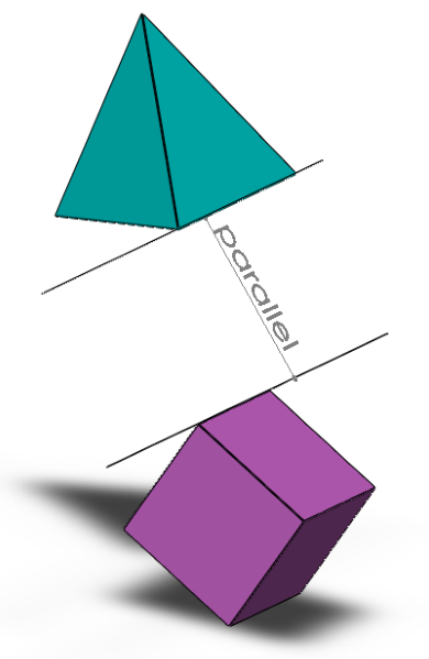
We use the four basic building blocks just presented to complete the development of the infinitesimal theory. In this section, we present the rows of the rigidity matrix associated with each of the 21 body-and-cad constraints. In all figures, body is represented by the green tetrahedron and body by the purple cube.
4.1 Angular constraints
Angular constraints may be parallel, perpendicular or arbitrary fixed angular constraints; see Figures 5–7 for depictions of line-line, line-plane, and plane-plane angular constraints.


We now formally define the functions for describing angular constraints.
- •
Line-line parallel: maps an edge to a triple so that the lines and affixed to bodies and , respectively, are constrained to remain parallel to each other.
- •
Line-line perpendicular: maps an edge to a pair so that the lines and affixed to bodies and , respectively, are constrained to remain perpendicular to each other.
- •
Line-line fixed angular: maps an edge to a triple so that the lines and affixed to bodies and , respectively, are constrained to maintain the angle between them.
- •
Line-plane parallel: maps an edge to a pair so that the line and plane affixed to bodies and , respectively, are constrained to remain parallel to each other.
- •
Line-plane perpendicular: maps an edge to a pair so that the line and plane affixed to bodies and , respectively, are constrained to remain perpendicular to each other.
- •
Line-plane fixed angular: maps an edge to a triple so that the line and plane affixed to bodies and , respectively, are constrained to maintain the angle between them.
- •
Plane-plane parallel: maps an edge to a triple so that the planes and affixed to bodies and , respectively, are constrained to remain parallel to each other.
- •
Plane-plane perpendicular: maps an edge to a pair so that the planes and affixed to bodies and , respectively, are constrained to remain perpendicular to each other.
- •
Plane-plane fixed angular: maps an edge to a triple so that the planes and affixed to bodies and , respectively, are constrained to maintain the angle between them.
It is straightforward that the line-line angular constraints (perpendicular, fixed angular and parallel) are expressed by the two basic angular building blocks. We observe that the line-plane and plane-plane angular constraints reduce to them as follows.
- •
Line-plane parallel: Reduces to line-line non-parallel fixed angular using the normal to the plane.
- •
Line-plane perpendicular: Reduces to line-line parallel using the normal to the plane.
- •
Line-plane fixed angular: Reduces to line-line non-parallel fixed angular using the normal to the plane.
- •
Plane-plane parallel: Reduces to line-line parallel using the planes’ normal.
- •
Plane-plane perpendicular: Reduces to line-line non-parallel fixed angular using the planes’ normals.
- •
Plane-plane fixed angular: Reduces to line-line non-parallel fixed angular using the planes’ normals.
4.2 Blind constraints
The remaining coincidence and distance constraints reduce to some combination of basic angular and basic blind constraints from Section 3.3. We consider them in the following order: point-point, point-line, point-plane, line-line, line-plane and plane-plane. Since a point-point distance constraint (Figure 8b)) is a bar (see [30, 34]), we consider only the point-point coincidence constraint.


The function maps an edge to a point so that it is constrained to lie on bodies and simultaneously.
Then the point-point coincidence constraint (Figure 8a) is infinitesimally maintained if the relative velocity of is exactly 0. Since and , then the relative screw is defined by , where and . Therefore, the constraint is infinitesimally maintained if and only if ’s infinitesimal velocity , i.e.,
if and only if
| (4.1) | |||||
| (4.2) | |||||
| (4.3) |
Thus, a point-point coincidence constraint corresponds to 3 rows in the rigidity matrix:


Point-line coincidence (Figure 9a): The function maps an edge to a pair so that point affixed to body is constrained to lie on the line affixed to body .
The point-line coincidence constraint is infinitesimally maintained by using 2 primitive blind constraints from Equations 3.7 and 3.8 to express that the relative velocity of lies in the same direction as :
| (4.4) | |||||
| (4.5) |
Thus, a point-line coincidence constraint corresponds to 2 rows in the rigidity matrix:
Point-line distance (Figure 9b): The function maps an edge to a triple so that point affixed to body is constrained to lie a distance from the line affixed to body .
Let be the perpendicular direction from the line to . Then the point-line distance constraint is infinitesimally maintained using 1 primitive blind constraint from Equation 3.6 to express that the relative velocity of is orthogonal to :
| (4.6) |
Thus, a point-line distance constraint corresponds to one row in the rigidity matrix:


Point-plane coincidence (Figure 10a): The function maps an edge to a pair so that the point affixed to body is constrained to lie in the plane affixed to body .
The point-plane coincidence constraint is infinitesimally maintained using Equation 3.6 to express that the relative velocity of remains in the plane:
| (4.7) |
Thus, a point-plane coincidence constraint corresponds to one row in the rigidity matrix:
Point-plane distance (Figure 10b): The function maps an edge to a triple so that the point affixed to body is constrained to lie a distance from the plane affixed to body .
The point-plane distance constraint is infinitesimally maintained by using Equation 3.6 to express that the relative velocity of remains parallel to the plane:
| (4.8) |
Thus, a point-plane coincidence constraint corresponds to one row in the rigidity matrix:


Line-line coincidence (Figure 11a): The function maps an edge to a pair so that the line is constrained to be affixed to bodies and simultaneously.
We place a line-line parallel angular constraint, resulting in 2 primitive angular constraints from Equations 3.2 and 3.3:
| (4.9) | |||
| (4.10) |
Then, to maintain coincidence, associate 2 primitive blind constraints from Equations 3.7 and 3.8 to force the relative velocity of to lie along :
| (4.11) | |||||
| (4.12) |
These 4 equations maintain the line-line coincidence constraint infinitesimally and correspond to 4 rows in the rigidity matrix:
Line-line distance (Figure 11b): The function maps an edge to a triple so that the lines and affixed to bodies and , respectively, are constrained to lie a distance from each other.
Let be the point on the line closest to the line . Then the line-line distance constraint is infinitesimally maintained if the relative velocity of is orthogonal to the direction perpendicular to both lines. In other words, must lie in the plane defined by the point and normal direction . By substituting and into Equation 3.6, we obtain the linear equation
| (4.13) |
associating one blind primitive constraint. This corresponds to one row in the rigidity matrix:


Line-plane coincidence (Figure 12a): The function maps an edge to a pair so that the line affixed to body is constrained to lie in the plane affixed to body .
The line-plane coincidence constraint is infinitesimally maintained using a primitive angular line-plane parallel constraint from Equation 3.1:
| (4.14) |
In addition, a primitive blind constraint from Equation 3.6 forces the relative velocity of to remain in the plane:
| (4.15) |
Thus, a line-plane coincidence constraint corresponds to 2 rows in the rigidity matrix:
Line-plane distance (Figure 12b): The function maps an edge to a triple so that the line affixed to body is constrained to lie a distance from the plane affixed to body .
The line-plane distance constraint is maintained infinitesimally by using the same equations as for the line-plane coincidence constraint: a primitive angular line-plane parallel constraint from Equation 3.1:
| (4.16) |
In addition, a primitive blind constraint from Equation 3.6 forces the relative velocity of to remain parallel to the plane:
| (4.17) |
Thus, a line-plane distance constraint corresponds to 2 rows in the rigidity matrix:


Plane-plane coincidence (Figure 13a): The function maps an edge to the pair so that the plane is constrained to be affixed to both bodies and simultaneously.
We place a plane-plane parallel angular constraint, resulting in 2 primitive angular constraints from Equations 3.2 and 3.3:
| (4.18) | |||
| (4.19) |
Then, to maintain coincidence, place a primitive blind constraint by using Equation 3.6 to force the relative velocity of to remain in the plane:
| (4.20) |
Thus, a plane-plane coincidence corresponds to 3 rows in the rigidity matrix:
Plane-plane distance (Figure 13b): The function maps an edge to a quadruple so that the planes and affixed to bodies and , respectively, are constrained to have the distance between them.
Maintaining the plane-plane distance infinitesimally reduces to the same linear equations as for plane-plane coincidence. We place a plane-plane parallel angular constraint, resulting in 2 primitive angular constraints from Equations 3.2 and 3.3 along with a primitive blind constraint using Equation 3.6 to force the relative velocity of to remain parallel to the plane:
| (4.21) | |||
| (4.22) |
| (4.23) |
Thus, a plane-plane distance constraint corresponds to 3 rows in the rigidity matrix:
4.2.1 Example
To help the reader, we complete the formalization of the dice example depicted in Figures 2 and 3. We assume that the -axis lies along the base of the dice in the direction of Face , with the -plane parallel to Face .
Then the framework is described by the functions:
- •
- •
- •
- •
Since the example only uses four types of constraints, we omit the description of the remaining functions.
For each edge, we construct the associated rows in the rigidity matrix, resulting in the following:
4.3 Summary of infinitesimal theory
We have now completed the development of the infinitesimal theory for body-and-cad rigidity. Table 1 summarizes the associations for each constraint to the number of primitive angular and blind constraints. As an example of how to read the table, the last two columns (corresponding to plane) of row 3 (corresponding to coincidence under line) indicate that a line-plane coincidence constraint reduces to 1 angular and 1 blind primitive constraint. In the next section, we identify a combinatorial property based on the shape of the rigidity matrix.
| point | line | plane | ||||
| angular | blind | angular | blind | angular | blind | |
| point | ||||||
| coincidence | 0 | 3 | 0 | 2 | 0 | 1 |
| distance | 0 | 1 | 0 | 1 | 0 | 1 |
| line | ||||||
| coincidence | 2 | 2 | 1 | 1 | ||
| distance | 0 | 1 | 1 | 1 | ||
| parallel | 2 | 0 | 1 | 0 | ||
| perpendicular | 1 | 0 | 2 | 0 | ||
| fixed angular | 1 | 0 | 1 | 0 | ||
| plane | ||||||
| coincidence | 2 | 1 | ||||
| distance | 2 | 1 | ||||
| parallel | 2 | 0 | ||||
| perpendicular | 1 | 0 | ||||
| fixed angular | 1 | 0 | ||||
5 Combinatorics
Now we address the question of combinatorially characterizing when a body-and-cad rigidity matrix is generically independent, i.e., the rank function drops only on a measure-zero set of possible entries. The shape of the rigidity matrix leads to a natural property that we call nested sparsity. We show that nested sparsity is a necessary condition for body-and-cad rigidity and prove by a counterexample that it is insufficient.
Nested sparsity. A graph on vertices is -sparse if every subset of vertices spans at most edges; it is tight if, in addition, it spans total edges.
Let be a graph with its edge set colored into red and black edges, corresponding to and , respectively. We say that is -nested sparse if it is -sparse and is -sparse; the graph is -nested tight if, in addition, is -tight. Note that nested sparsity only makes sense when -sparsity is more restrictive than -sparsity.
Primitive cad graphs. Given a cad graph , we define the primitive cad graph to be the multigraph obtained by assigning vertices to bodies and constraints to disjoint edge sets and , corresponding respectively to primitive angular and blind constraints. For each edge with type , associate primitive angular constraints to edges in and primitive blind constraints to edges in as described in Table 1. Figure 14 depicts the primitive cad graph associated with the dice example from Figure 2, whose cad graph is depicted in Figure 3.
Theorem 5.1.
Let be the primitive cad graph associated to a body-and-cad framework, where and correspond to primitive angular and blind constraints, respectively. Then -nested tightness is a necessary condition for generic minimal body-and-cad rigidity.
Proof.
Let be the rigidity matrix associated with . Reorder the columns so that the first columns correspond to the elements of the screws and the last columns correspond to the elements. Reorder the rows to have the rows corresponding to primitive angular constraints first; since these rows have all 0s in the last columns, we simply consider the submatrix defined by these rows and the first columns. Then it is clear that -sparsity is necessary on . To see that -sparsity is necessary, we note that the 3-dimensional space of trivial motions of (infinitesimal rotations) is a subspace of the kernel of . These are defined by the basis , where is the vector obtained by copies of , is the vector obtained by copies of , and is the vector obtained by copies of . Similarly, for the overall -sparsity, note that we have a 6-dimensional space of trivial motions of (infinitesimal rigid body motions), defined by the basis , where simply appends zeros to ; is the vector obtained by copies of , is the vector obtained by copies of , and is the vector obtained by copies of . ∎
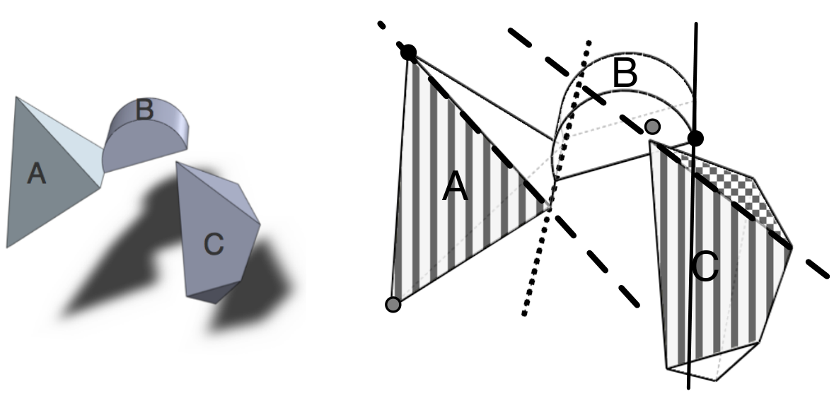

Counterexample. We now show that -nested sparsity is not sufficient for body-and-cad rigidity. The example in Figure 15 depicts a flexible structure whose associated graph is -nested tight. It is composed of 3 bodies and ; Figure 15a depicts the constraints. The structure has one degree of freedom, as indicated by the arrows in Figure 15b. The associated primitive cad graph is shown in Figure 15c; the reader may check that it is -nested tight.
6 Algorithms for nested sparsity
In the previous section, we defined nested sparsity, proving that is a necessary, but not sufficient, condition for body-and-cad rigidity. We now examine the algorithmic aspects of nested sparsity.
We first observe that nested sparsity is not matroidal, as seen by the example for -nested sparsity in Figure 16. However, for certain values of and , nested sparsity is the intersection of two matroids.
Theorem 6.1.
[31] When , for , nested sparsity is the intersection of two matroids.
Proof.
Define the ground set to be the complete graph ; the edges of the graph are colored red and black, with black edge multiplicity and red edge multiplicity. Let be the bases of the -sparsity matroid; then -nested sparsity is the intersection of the following two matroids, defined by their bases:
- 1.
, bases in the -sparsity matroid when edge color is disregarded.
- 2.
, bases in the red -sparsity matroid padded with full edge multiplicity of the black edges.
∎
As a consequence, when , the matroid intersection algorithm of Edmonds [4] can be used to solve the Decision (is a graph nested sparse?), Extraction (given an input graph, extract a maximum-sized nested sparse subgraph) and Components (given an input graph, extract its maximal vertex sets that span nested tight subgraphs) problems.
Edmonds’ algorithm outputs a maximum-sized set of edges that are independent in both matroids and requires an oracle to test for independence in each matroid. For the oracles, we use the pebble games algorithms of [14], a family of algorithms parametrized by two constants and ; the -pebble game characterizes -sparsity. In particular, the -pebble game takes a graph as input and can be run in two modes: the Decision mode returns “yes” if the input graph is -sparse, and the Components mode returns the maximal vertex sets that span -tight subgraphs. Algorithm 1 gives a more detailed description of how Edmonds’ matroid intersection algorithm is used to solve problems for nested sparsity.
Algorithm 1.
-nested sparsity: Decision, Extraction and Components
Input: A graph and constants , where
for .
Method:
1.
Run Edmonds’ matroid intersection algorithm [4] on
for the two matroids and ,
as defined in the proof of Theorem 6.1.
When the algorithm performs independence queries on a set of edges ,
(a)
For the matroid ,
play the -pebble game on the input in Decision mode, which
returns “yes” if it is -sparse
(b)
For the matroid ,
play the -pebble game on the input in Decision mode, which
returns “yes” if it is -sparse
2.
Edmonds’ algorithm returns a set that is of maximum size, where
is -nested sparse.
3.
Output:
•
For Decision, “yes” if and no otherwise.
•
For Extraction, .
•
For Components, play the -pebble game in Components mode
on and
output the components returned by the pebble game.
Complexity analysis. Edmonds’ algorithm queries the oracles times, where is the number of elements in the ground set and is the smaller rank of the two matroids. For nested sparsity, on a graph with vertices and edges, both matroids have rank . Therefore, Edmonds’ algorithm requires oracle queries. The pebble game algorithms require time, resulting in total complexity for Algorithm 1. We note that, using the recent matroid intersection algorithm of Harvey [8], a more efficient running time of , where is the matrix multiplication exponent, can be obtained for nested sparsity.
7 Conclusions
Constraint-based CAD software contains a rich set of geometric constraints. Motivated by their applications, we have initiated the study of body-and-cad rigidity by identifying a class of constraints amenable to rigidity-theoretical investigation and developing their infinitesimal theory. The shape of the rigidity matrix naturally led to the study of -nested sparsity, a necessary, but not sufficient, condition for body-and-cad rigidity. The polynomial time algorithm we presented for testing this condition may have practical applications as a filter for finding rigid components in a CAD environment, providing informative feedback to the user.
Applications. The results presented can be applied to a larger set of CAD constraints via simple reductions. In particular, it is easy to establish the following reductions:
- •
Sphere-sphere tangency: Reduces to point-point distance using the sphere centers and the sum of the radii.
- •
Sphere-plane tangency: Reduces to point-plane distance using the sphere center, the plane and the sphere radius.
- •
Sphere-line tangency: Reduces to point-line distance using the sphere center, the line and the sphere radius.
- •
Sphere-point coincidence: Reduces to point-point distance using the sphere center, the point and the sphere radius.
Analogous reductions can be applied when considering cylinders instead of spheres by substituting the cylinder’s center axis for the sphere’s center point.
Future directions. It remains an open problem to find a combinatorial characterization for generic body-and-cad rigidity. We anticipate the study of some of the constraints introduced here may prove more tractable than classical 3D bar-and-joint rigidity. A full combinatorial characterization for angular constraints appears in [16, 13]. However, we observe that finding a complete characterization may require overcoming well-known obstacles such as detecting dependencies in 3D bar-and-joint, 2D points-and-angles, 2D circles-and-angles, and 2D point-line incidence constraint systems.
Analogous body-and-cad structures for 2D consist of rigid bodies with pairwise coincidence (point-point, point-line and line-line), angular (line-line) and distance (point-point, point-line and line-line) constraints identified between points and lines rigidly attached to bodies. The development of the rigidity matrix is a straightforward extension of this work. The interesting question, which remains future work, is a full combinatorial characterization.
References
- [1] S. R. Ball. A Treatise on the Theory of Screws. Cambridge University Press, Cambridge, 1900.
- [2] H. Crapo and W. Whiteley. The statics of frameworks and movements of panel structures, a geometric introduction. Structural Topology, 6:43–82, 1982.
- [3] Dassault Systèmes. Solidworks: 3d mechanical design and 3d CAD software, 2010. http://www.solidworks.com/.
- [4] J. Edmonds. Matroid intersection. Annals of Discrete Mathematics, 4:39–49, 1979.
- [5] X.-S. Gao, D. Lei, Q. Liao, and G.-F. Zhang. Generalized stewart platforms and their direct kinematics. IEEE Trans. Robotics, 21:141–151, 2005.
- [6] X.-S. Gao, Q. Lin, and G.-F. Zhang. A c-tree decomposition algorithm for 2d and 3d geometric constraint solving. Computer-Aided Design, 38(1):1–13, 2006.
- [7] J. Graver, B. Servatius, and H. Servatius. Combinatorial rigidity. Graduate Studies in Mathematics. American Mathematical Society, 1993.
- [8] N. J. A. Harvey. Algebraic algorithms for matching and matroid problems. SIAM J. Comput., 39(2):679–702, 2009.
- [9] C. M. Hoffmann, A. Lomonosov, and M. Sitharam. Decomposition plans for geometric constraint problems, part II: New algorithms. Journal of Symbolic Computation, 31(4):409–427, 2001.
- [10] C. M. Hoffmann, A. Lomonosov, and M. Sitharam. Decomposition plans for geometric constraint systems, part I: performance measures for CAD. Journal of Symbolic Computation, 31(4):367–408, 2001.
- [11] C. Jermann, G. Trombettoni, B. Neveu, and P. Mathis. Decomposition of geometric constraint systems: a survey. Int. J. Comput. Geometry Appl., 16(5-6):379–414, 2006.
- [12] G. Laman. On graphs and rigidity of plane skeletal structures. Journal of Engineering Mathematics, 4:331–340, 1970.
- [13] A. Lee. Geometric Constraint Systems with Applications in CAD and Biology. PhD thesis, University of Massachusetts Amherst, May 2008.
- [14] A. Lee and I. Streinu. Pebble game algorithms and sparse graphs. Discrete Mathematics, 308(8):1425–1437, April 2008.
- [15] A. Lee, I. Streinu, and L. Theran. Graded sparse graphs and matroids. Journal of Universal Computer Science, 13(11):1671–1679, 2007.
- [16] A. Lee-St. John and I. Streinu. Angular rigidity in 3d: combinatorial characterizations and algorithms. In Proc. 21st Canadian Conf. Comp. Geometry (CCCG’09). Univ. British Columbia, August 2009.
- [17] H. Li and Y. Wu. Automated short proof generation for projective geometric theorems with Cayley and bracket algebras: I. incidence geometry. J. Symb. Comput., 36(5):717–762, 2003.
- [18] J. C. Maxwell. On the calculation of the equilibrium and stiffness of frames. Philos. Mag., 27:294, 1864.
- [19] D. Michelucci and P. Schreck. Incidence constraints: a combinatorial approach. International Journal of Computational Geometry & Applications, 16(5-6):443–460, 2006.
- [20] R. Plateaux, O. Penas, F. Mhenni, J.-Y. Choley, and A. Riviere. Introduction of the 3d geometrical constraints in Modelica. Proceedings of the 7th International Modelica Conference, Como, Italy, 2009.
- [21] F. Saliola and W. Whiteley. Constraining plane configurations in CAD: Circles, lines, and angles in the plane. SIAM Journal on Discrete Mathematics, 18(2):246–271, 2004.
- [22] J. M. Selig. Geometrical Methods in Robotics. Springer-Verlag New York, Inc., Secaucus, NJ, USA, 1996.
- [23] P. Serre, M. Moinet, and A. Clement. Declaration and specification of a geometrical part in the language of geometric algebra. Advanced Mathematical and Computational Tools in Metrology and Testing VIII, 78:298–308, 2009.
- [24] B. Servatius and W. Whiteley. Constraining plane configurations in CAD: Combinatorics of directions and lengths. SIAM Journal on Discrete Mathematics, 12(1):136–153, 1999.
- [25] M. Sitharam. Combinatorial approaches to geometric constraint solving: Problems, progress, and directions. In R. Janardan, M. Smid, and D. Dutta, editors, Geometric and algorithmic aspects of computer-aided design and manufacturing, volume 67 of DIMACS Ser. in Discrete Math. and Theoret. Comp. Sci., pages 117–163, Providence, RI, 2005. AMS.
- [26] M. Sitharam. Well-formed systems of point incidences for resolving collections of rigid bodies. Int. J. Comput. Geometry Appl., 16(5-6):591–615, 2006.
- [27] M. Sitharam, J. Peters, and Y. Zhou. Optimized parametrization of systems of incidences between rigid bodies. Journal of Symbolic Computation, 45(4):481–498, April 2010.
- [28] M. Sitharam, Y. Zhou, and J. Peters. Reconciling conflicting combinatorial preprocessors for geometric constraint systems. To appear in: International Journal of Computational Geometry and Applications, 2010.
- [29] I. Streinu and L. Theran. Sparse hypergraphs and pebble game algorithms. European Journal of Combinatorics, 30(8):1944–1964, November 2009.
- [30] T.-S. Tay. Rigidity of multigraphs I: linking rigid bodies in n-space. Journal of Combinatorial Theory Series, B 26:95–112, 1984.
- [31] L. Theran. Personal communication, 2007.
- [32] N. White. Grassmann-Cayley algebra and robotics. Journal of Intelligent and Robotics Systems, 11:91–107, 1994.
- [33] N. White. Geometric applications of the Grassmann-Cayley algebra. In J. E. Goodman and J. O’Rourke, editors, Handbook of Discrete and Computational Geometry, CRC Press, 1997. 1997.
- [34] N. White and W. Whiteley. The algebraic geometry of motions of bar-and-body frameworks. SIAM Journal of Algebraic Discrete Methods, 8:1–32, 1987.
- [35] W. Whiteley. A matroid on hypergraphs, with applications in scene analysis and geometry. Discrete and Computational Geometry, 4:75–95, 1989.
- [36] W. Whiteley. Some matroids from discrete applied geometry. In J. Bonin, J. G. Oxley, and B. Servatius, editors, Matroid Theory, volume 197 of Contemporary Mathematics, pages 171–311. American Mathematical Society, 1996.
- [37] Y. Zhou. Combinatorial Decomposition, Generic Independence and Algebraic Complexity of Geometric Constraints Systems: Applications in Biology and Engineering. PhD thesis, University of Florida, 2006.