OSU-HEP-10-05
June 5, 2010
Two–Loop Neutrino Mass Generation
through Leptoquarks
K.S. Babu** * Email: babu@okstate.edu and J. Julio†† † julio.julio@okstate.edu
aDepartment of Physics
Oklahoma State University
Stillwater, OK 74078, USA
Abstract
We present a new model of radiative neutrino mass generation wherein TeV scale leptoguark scalars induce tiny neutrino masses as two–loop radiative corrections. The neutrino oscillation parameter is predicted to be close to the current experimental limit within the model. Rare lepton flavor violating processes mediated by leptoquarks have an interesting pattern: may be suppressed, while and conversion in nuclei are within reach of the next generation experiments. New CP violating contributions to mixing via leptoquark box diagrams are in a range that can explain the recently reported discrepancy with the standard model. decays mediated by leptoquarks brings theory and experiment closer, removing an observed anomaly. Muon receives new positive contributions, which can resolve the discrepancy between theory and experiment. The leptoquarks of the model are accessible to the LHC, and their decay branching ratios probe neutrino oscillation parameters.
1 Introduction
It has now been firmly established that neutrinos have tiny masses and that oscillation occurs between different flavors. The standard paradigm that explains the small masses is the seesaw mechanism [1], which generates an effective dimension–5 operator , suppressed by the mass scale of the heavy right–handed neutrino. Oscillation data suggests that in this scenario , which is well beyond the reach of foreseeable experiments for direct scrutiny. One has to rely on other indirect hints, such as charged lepton flavor violation in a supersymmetric context, in order to falsify this theory.
An interesting alternative to the high scale seesaw mechanism is to induce small neutrino masses at the loop level. The smallness of neutrino masses can be understood as originating from loop and chirality suppression factors. The simplest among this class of models is the Zee model [3] where neutrino masses are induced as one–loop radiative corrections arising from the exchange of charged scalar bosons. The effective operator in this model is . To convert this to neutrino mass, a loop diagram is necessary.11 1 This model is now excluded by neutrino oscillation data (see Ref. [4]). In a second class of models, neutrino masses arise as two–loop radiative corrections via the exchange of singly and doubly charged scalars [5, 6]. The effective operator of these models is . This model is compatible with neutrino oscillation data. Phenomenology of these models has been studied in Ref. [7].
A classification of low dimensional effective lepton number violating operators that can lead to neutrino masses has been given in Ref. [8]. Among these is an operator labeled :
| (1) |
where are indices, with the family indices suppressed. It is the purpose of this paper to develop a renormalizable model that generates . We will show that such a model can be consistently constructed, with a variety of testable predictions.
Operator is most directly induced by the exchange of scalar leptoquarks.22 2 Neutrino mass generation at the one-loop level by leptoquark exchange has been studied in Ref. [9]. Neutrino mass generation at the two–loop level in the supersymmetric standard model with specific –parity violating couplings has been studied in Ref. [10]. For neutrino mass generation the two quark fields and the charged lepton field in will have to be removed, which implies that the masses arise at the two–loop level. The order of magnitude of the induced neutrino masses is
| (2) |
where is a dimensionful coefficient of a cubic scalar coupling, and GeV is the electroweak vacuum expectation value (VEV). In order to generate eV, it is clear that must be of order TeV, which would be within reach of the LHC.
TeV scale leptoquarks can mediate a variety of flavor changing processes. We have examined these constraints and found the neutrino mass generation to be self-consistent. Our findings include several interesting features: (i) may be suppressed, because of a GIM–like cancelation, but and conversion nuclei are within reach of the next generation of experiments. (ii) There is a new CP violating contribution mediated by leptoquark box diagrams in mixing, which can nicely fit the recently reported dimuon anomaly by the DØ collaboration. (iii) The 2 discrepancy between theory and experiment in the leptonic decay of mesons can be explained in the model, owing to new contributions from the leptoquarks. (iv) Muon receives new positive contributions which can resolve the theoretical anomaly there. (v) Neutrino oscillation parameters can be probed in the branching ratios of the leptoquarks. (vi) The leptoquark masses are constrained to be less than a few TeV, which should make them accessible to the LHC.
This paper is organized as follows. In Section 2 we discuss the model leading to two–loop neutrino mass generation and obtain the constraints placed on the oscillation parameters. The constraints from rare processes such as and are presented in Section 3. In Sec. 4 we discuss the collider signals of leptoquarks, and in Sec. 5 we conclude.
2 Model of two–loop neutrino mass generation
In this section we present our model of two–loop neutrino mass generation, and derive restrictions on the model parameters from neutrino oscillation data. Constraints from rare processes, discussed in Sec. 3, will be used to demonstrate the viability of the model and its predictions for neutrino oscillations.
2.1 Model
The gauge symmetry of our model is the same as the standard model (SM), . In addition to the SM Higgs doublet , the scalar sector consists of the following leptoquark multiplets:
| (3) |
In general, addition of leptoquarks into the theory can cause baryon number () violating interactions, we forbid them by assuming that is globally conserved. The leptoquarks have the following Yukawa interactions:
| (4) |
Here are family indices and are indices. Note that these Yukawa couplings conserve both baryon number and lepton number (), as can be seen by assigning ( charges of to and to . The couplings , allowed by the gauge symmetry are forbidden by , and the couplings , allowed by the gauge symmetry as well as are forbidden by lepton number symmetry, which is assumed to be broken only by soft terms.33 3 The couplings of course do not mediate rapid proton decay, however, their simultaneous presence with the couplings of Eq. (4) would lead to severe restrictions on , since the successful structure of the SM will then be drastically altered [11]. Although not essential, we prefer to set these couplings to zero by symmetry. This breaking of by two units occurs softly via a cubic term in the scalar potential:
| (5) |
The simultaneous presence of Eqs. (4) and (5) would imply that neutrino masses will be generated at the loop level, as they lead to to the effective dimension 7 operator [8], once the heavy leptoquark fields are integrated out.
The Lagrangian relevant for neutrino mass generation in component form is
| (6) |
Once the neutral component of the SM Higgs doublet acquires a vacuum expectation value (VEV) GeV, the cubic term in the scalar potential will generate mixing between and leptoquarks, with a mass matrix given by
The parameter can be made real by redefining the leptoquark fields. We diagonalize this matrix to obtain the leptoquark mass eigenstates through
where with the angle given by
| (17) |
The squared masses of are given by
| (18) |
with .
2.2 Two–loop neutrino mass diagrams
Since lepton number violation occurs only when all three terms of Eq. (6) are simultaneously present, neutrino masses are generated in the model only at the two–loop level. The relevant diagrams, which involve the exchange of leptoquarks and a boson, are shown in Fig. 1. We have evaluated these diagrams in the Feynman gauge. In this gauge, the unphysical charged Higgs boson exchange has to be kept. Interestingly, this set of charged Higgs diagrams add up to zero for the neutrino mass. The underlying reason for this result is that in the SM, both the up–type quark masses and the down–type quark masses are generated from the same Higgs doublet. Consequently the charged Higgs boson Yukawa couplings to the up–type quark has a relative minus sign compared to its Yukawa couplings to the down–type quarks, as given in the interaction Lagrangian
| (19) |
Here is the CKM matrix, and and are the diagonal mass matrices for the up and down quarks. When combined with Fig. 1b, this relative minus sign implies zero net contribution to the neutrino mass from the charged Higgs boson exchange. In Fig. 1b, the vertex is a sum of two contributions, one where chirality flip occurs in the line, and the other where it occurs in the line. These two contributions exactly cancel, see Eq. (19).


Straightforward evaluation of the leptoquark– exchange diagrams gives the neutrino mass matrix as:
| (20) |
Here are the (normalized) diagonal mass matrices for up quarks, down quarks, and charged leptons:
| (21) |
The overall scale is given by
| (22) |
where is the lighter of the two charge leptoquark mass and is a color factor.
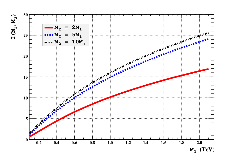
The dimensionless two–loop integral depends on the two leptoquark masses, the boson mass, , and the up–type quark masses , down–type quark masses and charged lepton masses , and is defined as
| (23) | |||||
In the asymptotic limit, i.e., in the limit of , the integral becomes independent of the flavor indices and takes the form
| (24) |
When the index is not equal to 3 (corresponding to no top quark inside the loop), this asymptotic expression well approximates the exact integral. The integral corresponding to top quark inside the loop obtained numerically is shown in Fig. 2 as a function of . Here we have taken the running top quark mass GeV. It will turn out that will enter into the dominant source for neutrino masses.
We now proceed to write down the neutrino mass matrix explicitly. First note that if the integral in Eq. (20) is flavor universal (as happens in the asymptotic limit as given in Eq. (24)), or if is the only dominant contribution, can be written as
| (25) |
where is the flavor universal value of . Now, this equation can be expanded in power series in light fermion masses. Combining constraints from flavor changing processes, we find, to an extremely good approximation, that the neutrino mass matrix is given by
Here we have used the following definition of parameters:
| (30) |
As expected, the leading contributions are proportional to , see the definition of in Eq. (22). One additional contribution, denoted as in the (3,3) entry of Eq. (2.2), can be important, for a very restricted range of parameters. This is in spite of the additional mass suppression factors that appears in , and occurs for the parameter choice and GeV. The Yukawa coupling combination appearing in is allowed to be order one, these couplings do not lead to excessive flavor violating processes even when the leptoquarks are light. ( couples to , and couples to , both of which are found to be rather un-constrained.) Contributions not shown in Eq. (2.2) have magnitudes eV, because of mass suppression factors and the constraints on the Yukawa couplings arising from rare processes mediated by the leptoquarks.
We shall consider the case for the most part of our analysis, but we shall also examine the special case where , which will be realized when the coupling takes anomalously small value and the leptoquark mass is less than about 500 GeV.
The zero in the (1,1) entry of Eq. (2.2) is highly suppressed. We find, using the lowest non-vanishing contribution from Eq. (25) for this entry to be
| (31) |
Now, unless takes values as large as , this entry will be negligible for neutrino masses. That possibility is however inconsistent with an acceptable fit to neutrino data on the one hand, and flavor violating constraints on the other. To see this, let us note that a good fit to neutrino data, discussed in more detail later in this section, requires and . Further, the leptoquark mass should not exceed about 10 TeV, or else the neutrino mass will be smaller than 0.05 eV, which would be inconsistent with the atmospheric oscillation data. For the same reason, , while allowed, would require the leptoquark mass to be much below a TeV. Then flavor violation constraints become important. conversion in nuclei sets an upper limit on the products and corresponding to a leptoquark mass of 300 GeV. When these limits are combined with the need to obtain the right magnitude for , we see that cannot be smaller than . Consequently the (1,1) entry of , given in Eq. (31), is much smaller than 0.01 eV. This of course means that contributions to neutrinoless double beta decay from light neutrino exchange is negligible. See however, other contributions to this process via the exchange of a leptoquark and boson in Fig. 10 discussed later, which turns out to be significant.
The other remarkable feature of the mass matrix in Eq. (25) is that, although it may not be obvious from its form, has nearly zero determinant when . This would imply that one of the neutrinos is essentially massless in the model for most of the parameter space. This can be seen by observing that only the top quark mass, and not the and quark masses, has entered into when is set to zero. In this case, each of the two terms in Eq. (25) has rank one, and the sum of the two terms has rank two, leaving the determinant to be zero. The first non-zero entry to the determinant in our expansion is found to be
| (32) | |||||
Again, with , , and (or equivalently ), the determinant will be much less than and thus to a high degree of accuracy. Note that cannot be less than , or else the neutrino mass scale will be too small.
2.3 Predictions for neutrino oscillations when
We turn now to the predictions of the model when , which is realized is much of the parameter space. Since in Eq. (2.2) has only four (complex) parameters, there are two predictions for neutrino masses and mixings. These are summarized below:
| (33) |
Here we have used the standard parametrization of the PMNS matrix. Furthermore, the two Majorana phases and (the phases of masses and respectively) are given by
| (34) |
with being a consequence of . These predictions have been obtained in the context of textures before (see Ref. [13]). Here we have derived them without resorting to textures.
To check the consistency of these predictions, we keep eV2, eV2 at their central values [14], and then vary in its allowed range. This gives from Eq. (33)
| (35) |
where the numbers correspond to the central value, and deviation in . This should be compared with the limit , at the level [14]. We see broad agreement, although should be very close to the current limit.

We can infer the values of in Eq. (2.2) from neutrino data. For this purpose we use the central values from neutrino data: eV2, eV2, along with , , and [14]. We obtain
| (36) |
The absolute values of are given in Fig. 3. We see that and . These values will directly affect the branching ratios of the leptoquarks, making a strong connection between collider physics and neutrino physics.
2.4 A special case with
It is interesting to see the constraints on the model when . This occurs for a small range of parameters when the leptoquark mass is less than about 500 GeV, and when . The latter condition can be satisfied when either or is much smaller than . Both of these couplings cannot be simultaneously very small, or else the (2,3) entry of will become unacceptably small.
When , we have the condition , see Eq. (2.2). Since in this case we reproduce a well known texture model [16, 17]. This limit of our model leads to the following predictions for and the phase parameters:
| (37) | |||||
| (38) |
This gives , which is within reach of the next generation long baseline neutrino oscillation experiments. This case requires the leptoquarks to be lighter than about 500 GeV, which are within reach of the LHC.
2.5 The case of
Forthecasewhenw ∼1M_νm_1a≡ m 1 m 2 cot^2θ_12θ_13w ∼1
2.6 Limit on the parameter
There are certain restrictions on the parameter that enters in the neutrino mass Lagrangian of Eq. (6). It is this term that is responsible for the mixing of with . Since the partner of does not mix with any other field, the term will induce new contributions to the electroweak parameter (or equivalently the parameter). This is because mixing via the term splits the masses of the doublet members. This mass-splitting must obey [12]
| (40) |
where for leptoquarks. In our model, apart from the term, there is a quartic scalar coupling, , which contributes to the mass, and not to the mass, causing a further splitting. The parameter in Eq. (40) is given by
| (41) |
where we have assumed that the two states are nearly degenerate. The two–loop induced neutrino mass is maximized when the mixing parameter . For this choice, one has the relations . When the leptoquark mass is well above 200 GeV, the contribution in Eq. (41), which is at most of order (200 GeV)2, can be neglected in relation to the term. In this case we obtain from Eq. (40) an upper limit on : . We shall use this constraint in deriving an upper limit on the leptoquark mass.
There are other reasons why cannot be arbitrarily large: the positivity of leptoquark squared mass (needed for color conservation) and the perturbativity of the theory. The first of these conditions implies, from Eq. (18), that
| (42) |
The second constraint emerges because induces negative quartic couplings for the three fields , and . These induced couplings cannot exceed the corresponding tree–level quartic couplings which can at most be of order one. Otherwise the theory would be non-perturbative, or electric charge and color would break in the minimum of the theory. We parameterize the effective quartic couplings of the three fields as
| (43) |
with . The 1–loop correction to these quartic couplings are shown in Fig. 4.44 4 For the term, there is a similar diagram generated by the SM quartic coupling. But here we focus on the diagrams generated by the term. By evaluating these diagrams we obtains for the effective couplings,
| (44) |
where the factor 3 in is a color factor. Since these effective couplings are negative, they must be smaller in magnitude compared to the corresponding tree level ones, otherwise the potential would become unbounded, suggesting instability of the vacuum. By demanding all these induced couplings to be less than one, so that the theory is perturbative with a stable vacuum, one can derive limits of . Of course, if the limit derived from Eq. (42) turns out to be more stringent, that will supersede the present limits.

For illustration, we consider a few simplified cases.
- •
. For and , the bound from Eq. (42) gives a more stringent limit, i.e. . For and the other masses the same as above, the more stringent limit comes from the , viz., .
- •
: In this case
(45) where is the smallest of and . For example, if , , and , .
- •
: In this case
(46) where . The choice of depends upon the value of and . For example, if and , one uses , so . On the other hand, if and , one uses , so .
2.7 Limit on leptoquark masses
The scaling of the neutrino mass with the LQ mass goes as . Since our neutrino mass matrix has a normal hierarchy structure, the neutrino mass scale should be around 0.02 eV. We shall assume that all the Yukawa couplings are bounded by 1, a requirement for perturbative treatment of the problem. As we have seen, a fit to the neutrino oscillation data requires . The maximum value of is realized for , corresponding to largest allowed LQ mass. From these considerations we arrive at a limit on the LQ mass of 12 TeV. If the leptoquarks are in the multi-TeV range, all three members should be nearly degenerate, from the requirement of and the parameter constraint. A slightly better limit can be derived on their masses from the rare process conversion in nuclei (see the next section for details). From the experimental limit on this process, one can derive the upper limit on as a function of mass. Since neutrino mass fitting requires to be of the same order for , one can also determine an upper limit on . Combining all of these, we obtain an upper limit of 10 TeV on .
There are lower limits on leptoquark mass from the Tevatron where they could be pair produced. The DØ and CDF experiments [15] have obtained limits on the second and the third generation leptoquarks of 316 GeV and 245 GeV respectively [15]. Since those experiments look for b-jets and missing energy, these bounds are strictly applicable for leptoquarks coupled to neutrinos. In our case, and have direct couplings to the neutrinos (the latter from mixing) for which the quoted limits apply. As for , being a member of the same doublet as , it should be nearly degenerate with , and thus the limits of Ref. [15] should apply to as well.
3 Constraints from rare processes
Since this model features lepton flavor (as well as total lepton number) violation, it is important to see how its parameters are constrained by the experimental data, especially those arising from rare decay processes that are forbidden in the SM. Here we derive a variety of limits on the couplings and as functions of the LQ masses. These limits should be (and have been) satisfied in the neutrino fits. The processes we shall consider are , , conversion in nuclei, , , mixing, mixing, mixing, decay, muon , decay, and neutrinoless double beta decay. The expected rates for several of these processes are found to be in the interesting range for the next generation of experiments.
3.1
The rare decay arises from a one–loop diagram. In the limit of , there are only three diagrams for this decay shown in Fig. 5. In general, the amplitude for this decay process can be written as [18]
| (47) |
where is the muon mass, is the photon momentum, and is the photon polarization vector. The effective couplings and are found to be (repeated indices implies summation)
| (48) |
where , ; and are the -th generation of up– and down–type quark masses respectively; and are and masses respectively; and and are the dimensionless functions given by [19, 20]
| (49) |
These expressions assume that the leptoquark mixing angle (see Eq. (17)) is zero. For non-zero , one can make the following replacement:
| (50) |
where , , and are defined in Eq. (18).

It is an excellent approximation to set the first and second generation quark masses to zero. The branching ratio for this decay is found to be
| (51) |
where is the fine structure constant. Constraints from other processes are presented in Table 1, where we have used the approximation .
An interesting feature of this analysis is that the couplings are only weakly constrained from these processes. This is owing to a GIM–like cancelation for the amplitude of this process from the two diagrams (Fig. 5). In the limit of down-type quark mass being zero, the two graphs exactly cancel. This cancelation occurs because the charge of the internal leptoquark () is twice as large and opposite in sign compared to the charge of of the internal down quark (. The amplitude of the graph where the photon is emitted from the scalar line is twice smaller compared to the one where the photon is emitted from the fermion line, leading to the cancelation. The non-canceling contribution is suppressed by a factor in the amplitude, which weakens the limit.
| Process | BR | Constraint |
|---|---|---|
3.2
These processes also occur at the one–loop level in our model (see Fig. 6). Here, there exist photon, –boson, and the SM Higgs–boson exchange diagrams, as well as box diagrams. The SM Higgs diagrams are suppressed by the electron mass, and thus highly suppressed and therefore ignored. Therefore, only the photon, –boson, and the box diagrams will be evaluated.
In the case of photon exchange, because the photon is now off-shell, and with the electron mass set to zero, the amplitude is given by
| (52) | |||||
where . and are the incoming muon and outgoing electron momenta respectively. The couplings and are found to be
| (53) |
where , , , and . The dimensionless functions and are given by [20]
| (54) |

For the boson exchange diagram, the leading contribution after ignoring terms suppressed by , with being leptoquarks mass, is
| (55) | |||||
where and . Since we set the first and second generation quark masses to zero (which is a good approximation), the effective couplings, and , are given by
| (56) |
with
| (57) |
For the box diagrams, the amplitude can be written as
| (58) | |||||
Here we have set all the quark masses to zero.
We now proceed to the calculation of the total amplitude. In the loop integral functions, , since the couplings are not constrained by , one needs to include all the diagrams mediated by boson, since the couplings may be of order one. However, since the –boson exchange contribution is suppressed by the the bottom quark mass, it can safely be ignored. On the other hand, the exchange is significant for mediated process with the top quark inside the loop. The electron mass has to be included in the calculation in order to avoid infrared singularity. The branching ratio is found to be
| (59) |
where we have introduced Hermitian parameters , given by
For heavy quarks inside the loop, the factors are in the agreement with [20].
Regarding the neutrino oscillation data, one needs the limit on the coupling constants that appear in Eq. (30). From the branching ratio above, in the assumption that there is no accidental cancelation among the various contributions, so that one can omit terms like or with , one gets, for a LQ mass of 1 TeV,
| (73) |
if and
| (74) |
if .
3.3 Conversion in the nuclei

Another lepton flavor violating process that may occur in this model is conversion in nuclei (). The interesting type is the so-called coherent conversion in which the nucleus does not change its initial state [21]. In this section we shall discuss the implications of our model in such processes. It turns out that there exist tree level diagrams in addition to the one–loop diagrams (Fig. 7). These two sets of diagrams probe different Yukawa couplings. The loop diagrams involve the same couplings that appear in the neutrino mass matrix, and has to be given special attention. These loop diagrams are similar to except the pair of up/down quark is attached to the photon and lines. Following [18], the branching ratio of this process is given by
| (75) | |||||
where and are the momentum and energy of the outgoing electron respectively, is the atomic number of the nucleus, is the mass number of the nucleus, is the effective atomic number defined in [22], is the nuclear matrix element defined in [18, 21, 22], is the muon capture rate of nucleus , and are defined as
| (76) |
Here and are the charges of the up– and down–quarks. As before, we can neglect terms proportional to and . The summary of constraints from this process is given in Table 2, with
| (77) | |||||
where and . Here we take .
| Element | BR | Constraint | ||
|---|---|---|---|---|
| 17.61 | 0.53 | |||
| 33.81 | 0.15 |
For , we get for LQ mass of 1 TeV, and which are slightly stronger than the constraints from . The tree–level diagrams alone give and . A new generation experiment called COMET has been proposed to reach a better sensitivity of [24]. There is also discussion of testing conversion at a future Fermilab experiment. The prospects for these experiments observing new physics are good within our model. This is true even if the MEG experiment [25] obtains negative results for the decay.55 5 There is a class of model where conversion is log–enhanced compared to , see Ref. [26].
We can use the bound from conversion and neutrino mass fitting to predict the minimum branching ratio for . Such a correlation is not possible for because of the GIM-like cancelation that occurs there, and the fact that is not constrained by neutrino data. Note that, (assuming that only the bottom quark mediates the process) cannot be smaller than for LQ mass of 300 GeV, or else the induced neutrino mass will be too small. Therefore, the smallest branching ratio for can be predicted which is presented in Fig. 8. We see that can be substantial for a significant part of the parameter space.

3.4 and decays
It turns out that some of the potentially large entries in the neutrino mass matrix are eliminated from the constraints from the decays and . These processes can be mediated by leptoquark at tree level. Here we ignore mixing and work in the flavor symmetric limit. The branching ratios for these processes are given by
| (78) |
We use and data from [12] to derive
| (79) |
3.5 Muon anomalous magnetic moment
The muon anomalous magnetic moment receives correction from the leptoquark exchange in our model and is given by
| (80) |
Again, for the same reason as in the case of , couplings are practically have no effects here. By comparing the new contributions with the anomaly in the experimental value, [27, 28], we see that this model can reduce or eliminate the discrepancy for order one values of the couplings and .
3.6 Upsilon Decay
Lepton number violating decay can set limit on the couplings . The decays we consider are and . The former is generated by the s-channel photon exchange and the latter is generated by the t-channel exchange. In our model the ratio of these two branching ratios is given by
| (81) |
where is the mass. The upper limit of this ratio is [29]. Therefore, we get less constrained value
| (82) |
3.7 decay
Another interesting feature of the leptoquarks is that they can mediate a lepton number violating decay: . Currently there is a discrepancy about level between the experimental value and theoretical predictions based on lattice evaluation of the decay constant . The LQ exchange can resolve the discrepancy. This issue has been studied in the framework of MSSM with broken -parity [27, 30] and in extensions of the standard model with leptoquarks [31]. It turns out that in this model this process occurs at tree level mediated by leptoquarks in addition to the SM process. Since the SM diagram leads to antineutrino final states, while the mediating processes result in neutrinos, there is no interference between the two.66 6 Analogous lepton number violating muon decay has been explored as an explanation of the LSND anomaly in Ref. [32]. We get
| (83) | |||||
where and are the mass and lifetime respectively while is the element of CKM matrix. Comparing results from lattice calculation, [33], and the experimental result, [34], we see that at present there is a 2 discrepancy. If this discrepancy prevails, there is a natural explanation in the present context. Assuming maximal mixing among the two charge leptoquarks, we obtain the constraint (corresponding to the central values of the decay constants and )
| (84) |
There is a similar contribution to the decay . From this process we find
| (85) |
By using experimental limits [12], one can derive
| (86) |
3.8 New CP violation in mixing
The leptoquarks of the model mediate meson–antimseon mixing via one–loop box diagrams shown in Fig. 9. There is special interest in this process for the system, as there are experimental hints for non–zero CP violation in this system. We find that the present model can nicely explain the new CP violation that would be needed in mixing, without generating unacceptable mixing in the , and systems.
The new effective Lagrangian for mixing in the model arising from the box diagrams of Fig. 9 is given by
| (87) |
The transition amplitude is given by
| (88) |
where and are the meson mass and decay constant respectively, while and are the bag parameter and the QCD correction factor evaluated at the scale GeV and their numerical values are and [35].

Recently the DØ collaboration has reported an excess in the like-sign dimuon asymmetry [36] defined as
| (89) |
where is the numbers of events containing two hadrons that decay semileptonically into two positive (negative) muons. Eq. (89) can be written as a linear combination of two asymmetries [37, 36]
| (90) |
where () is defined as [36]
| (91) |
In the SM, and [38], so that which is away from the current measurement (see Eq. (89)). A likely explanation is that there is a new source of CP violation in mixing, which can arise from leptoquarks, as given in Eq. (88).
The leptoquark contribution will modify the mass difference in the system [39]:
| (92) |
In our model, the new contribution is given by
| (93) |
The index is to be summed in Eq. (93), but in practice not all three lepton flavors can simultaneously be significant, owing to lepton flavor violating constraints. Therefore we focus on the contributions.
A global fit to the CKM mixing parameters, including the new DØ data on dimuons, finds [39] or {} as the best fit values. The leptoquark contributions will be maximal when , which is allowed in the model, and when the leptoquark mass is the smallest ( GeV). In this case for in order to satisfy lepton flavor violating constraints. A fit to the neutrino oscillation data requires all the () to be of the same order with corresponding to . In this case, conversion in nuclei sets a limit . Using this upper limit in Eq. (93), and using [40], we find . The phase is unconstrained, and can take the desired value of . These are in excellent agreement with the global fit of Ref. [39].
We need to point out that the leptoquark model could affect the absorptive part of the mixing amplitude [41]:77 7 We thank Amol Dighe for useful discussion on this point.
| (94) |
where is given by [41]
| (95) |
where is a kinematic function, as a function of . The numerical values of this function are for and . By using the same parameter values as for , we see that the new contribution can modify the SM value of the width difference by at most 2%. There is currently a 2 discrepancy in , which should be explained as a statistical fluctuation within our model.
Similar expressions hold for the mixing of other meson systems:
| (96) |
The factors are found by following the procedures given in Ref. [35] to be , with .
The limits on those couplings appearing in , , and mixings can be derived by using , , , , , and . They are found to be
| (97) |
These constraints are all consistent with acceptable generation of neutrino masses and mixings within the model.
3.9 Neutrinoless double beta decay
The light neutrino exchange contribution to neutrinoless double beta decay vanishes in our model, owing to the zero of the (1,1) entry in . However, it can proceed via the vector–scalar exchange process, which does not need a helicity flip of the neutrino [42]. The relevant diagram is shown in Fig. (10). The effective Lagrangian of that process after Fierz rearrangement is
| (98) |
where is the internal neutrino momentum. The first term is the scalar-pseudoscalar current and the second one is the tensor current, and the parameter is defined as
| (99) |
where is the leptoquarks mixing angle. Following Päs et al. [43], the constraint on is calculated by constructing nuclear matrix element in pn-QRPA model [44] and applying the result of half life, , obtained from Heidelberg-Moscow experiment [45]. A straightforward calculation gives
| (100) |
Here, both the scalar-pseudoscalar and tensor currents are taken into account. One sees that it is possible to observe neutrinoless double beta decay in the near future, even with hierarchical neutrino masses.

4 Collider signals
At hadron colliders, leptoquarks can be produced in pairs via quark-quark or gluon-gluon fusion and/or in association with lepton via quark-gluon fusion. The former depends on the QCD coupling constant and the latter depends on the and . The associated production may be important if the and are as large as electromagnetic coupling [46]. Since these couplings are constrained by rare processes such as neutrinoless double beta decay, it seems unlikely that single production will be dominant in our model. Therefore, here we focus on pair production of leptoquarks.
In pair production, each will decay to a charged lepton and a down quark with opposite charges. The resulting final state is two leptons and two jets. At the LHC with and mass of leptoquark equals to , the cross section is about fb [46], decreasing to fb for a LQ mass of 1 TeV. The dominant background for this process is final states from and production. For high leptoquark mass, only is dominant. LHC can probe this leptoquark mass up to with integrated luminosity of .
In pair production, there are two possible signals. First, each decays to up–quark and a lepton, leading to two lepton and two jets signal. Secondly, one decays to charged lepton and up quark and the other one decays to neutrino and a down–type quark, leading to one lepton plus jets plus missing energy. The first signature is similar to the case. The second one has dominant background coming from and production. In Ref. [46], it has been shown that LHC can probe this leptoquark mass up to with integrated luminosity of .
The decays of the leptoquark into will occur in the following ratios:
| (101) |
Measurement of any one of these branching ratios will determine the CP violating phase via Eq. (36). This can of course be cross checked in long baseline neutrino oscillation experiments, especially since is large. If two branching ratios in the decay of are measured, that will determine the phase in two different ways, allowing for another consistency check.
The leptoquarks , () which are linear combinations of and will decay into charged leptons in the following ratios:
| (102) |
Note that this result holds for both , independent of the mixing angle . Measuring this branching ratio will determine , providing another check for the model. Since numerically , we expect that at least one of the the will have in the final state dominantly. It should be noted that the decay will be suppressed, owing to constraints from . Of course, these fields also decay into . The lepton flavor composition in this mode would be near to impossible to determine.
5 Conclusion
In this paper we have presented a new two–loop neutrino mass generation model. This involves TeV scale leptoquarks, which can be directly tested at the LHC. The structure of the model is such that the neutrino mixing angle is predicted to be close to the current experimental limit of 0.05. The neutrino oscillation parameters are closely linked to the decay properties of the leptoquarks. By measuring the branching ratios of the LQ bosons, in this model, one is measuring CP violating phase of neutrino oscillations. These measurements also provide a number of cross checks by which the model can be falsified.
We have discussed various rare decay processes mediated by the LQ bosons. The process may very well be suppressed, owing to a GIM–like mechanism, while the decay and conversion in nuclei are within reach of the next generation experiments. A very interesting feature of the model is that the present hint of new physics contributions to CP violation in mixing fits rather well here, without conflicting other well-measured meson mixings. Neutrinoless double beta decay can occur via LQ exchange, even when the neutrino spectrum has a normal hierarchy. Near future experiments will have a lot to say on the consistency of the model.
Acknowledgment
This work is supported in part by US Department of Energy Grant Numbers DE-FG02-04ER41306 and DE-FG02-ER46140.
References
- [1] P. Minkowski, Phys. Lett. B67, 421 (1977); M. Gell-Mann, P. Ramond, and R. Slansky, in Supergravity, eds. D. Freedman et al., (North-Holland, Amsterdam, 1980); T. Yanagida, in Proceedings of the Workshop on Baryon Number in the Universe, eds. O. Sawada and A. Sugamoto, (KEK, 1979); R. Mohapatra and G. Senjanović, Phys. Rev. Lett. 44, 912 (1980).
- [2] A. Zee, Phys. Lett. B93, 389 (1980).
- [3] For phenomenological analyses see: A. Y. Smirnov and M. Tanimoto, Phys. Rev. D 55, 1665 (1997).
- [4] X. G. He, Eur. Phys. J. C 34, 371 (2004).
- [5] A. Zee, Nucl. Phys. B 264, 99 (1986).
- [6] K. S. Babu, Phys. Lett. B203, 132 (1988).
- [7] K. S. Babu and C. Macesanu, Phys. Rev. D 67, 073010 (2003); M. Nebot, J. F. Oliver, D. Palao, and A. Santamaria, Phys. Rev. D 77, 093013 (2008); D. Aristizabal Sierra and M. Hirsch, JHEP 0612, 052 (2006).
- [8] K. S. Babu and C. N. Leung, Nucl. Phys. B619, 667 (2001).
- [9] D. Aristizabal Sierra, M. Hirsch, and S. G. Kovalenko, Phys. Rev. D 77, 055011 (2008).
- [10] P. Dey, A. Kundu, B. Mukhopadhyaya, and S. Nandi, JHEP 0812, 100 (2008).
- [11] W. Buchmuller and D. Wyler, Phys. Lett. B 177, 377 (1986); W. Buchmuller, R. Ruckl, and D. Wyler, Phys. Lett. B 191, 442 (1987) [Erratum-ibid. B 448, 320 (1999)].
- [12] Particle Data Group, C. Amsler et al., Phys. Lett. B667, 1 (2008).
- [13] K. S. Babu, Y. Meng, and Z. Tavartkiladze, arXiv:0812.4419 [hep-ph] and references therein.
- [14] T. Schwetz, M. A. Tortola, and J. W. F. Valle, New J. Phys. 10, 113011 (2008).
- [15] V. M. Abazov et al. [D0 Collaboration], arXiv:1005.2222 [hep-ex]. D. E. Acosta et al. [CDF Collaboration], Phys. Rev. D 72, 051107 (2005); V. M. Abazov et al. [D0 Collaboration], Phys. Rev. D 71, 071104 (2005); A. Abulencia et al. [CDF Collaboration], Phys. Rev. D 73, 051102 (2006); V. M. Abazov et al. [D0 Collaboration], Phys. Lett. B 636, 183 (2006).
- [16] P. H. Frampton, S. L. Glashow, and D. Marfatia, Phys. Lett. B 536, 79 (2002).
- [17] Z. z. Xing, Phys. Lett. B 530, 159 (2002).
- [18] Y. Kuno and Y. Okada, Rev. Mod. Phys. 73, 151 (2001).
- [19] L. Lavoura, Eur. Phys. J. C 29, 191 (2003).
- [20] J. Hisano, T. Moroi, K. Tobe, and M. Yamaguchi, Phys. Rev. D 53, 2442 (1996); E. Arganda and M. J. Herrero, Phys. Rev. D 73, 055003 (2006); J. Hisano and D. Nomura, Phys. Rev. D 59, 116005 (1999).
- [21] A. Czarnecki, W. J. Marciano, and K. Melnikov, AIP Conf. Proc. 435, 409 (1998).
- [22] H. C. Chiang, E. Oset, T. S. Kosmas, A. Faessler, and J. D. Vergados, Nucl. Phys. A 559, 526 (1993).
- [23] M. Eckhause, R. J. Harris, and W. B. Shuler, Phys. Lett. 19, 348 (1965).
- [24] Y. G. Cui et al. [COMET Collaboration], KEK-2009-10, Jun 2009.
- [25] M. Grassi [MEG Collaboration], Nuovo Cim. 032C, 223 (2009).
- [26] M. Raidal and A. Santamaria, Phys. Lett. B 421, 250 (1998).
- [27] G. Bhattacharyya, K. B. Chatterjee, and S. Nandi, Nucl. Phys. B 831, 344 (2010).
- [28] J. Prades, Acta Phys. Polon. Supp. 3, 75 (2010).
- [29] W. Love et al., Phys. Rev. Lett. 101, 201601 (2008).
- [30] A. Kundu and S. Nandi, Phys. Rev. D 78, 015009 (2008).
- [31] B. A. Dobrescu and A. S. Kronfeld, Phys. Rev. Lett. 100, 241802 (2008); R. Benbrik and C. H. Chen, Phys. Lett. B 672, 172 (2009); I. Dorsner, S. Fajfer, J. F. Kamenik, and N. Kosnik, Phys. Lett. B 682, 67 (2009).
- [32] K. S. Babu and S. Pakvasa, arXiv:hep-ph/0204236.
- [33] E. Follana, C. T. H. Davies, G. P. Lepage, and J. Shigemitsu [HPQCD Collaboration and UKQCD Collaboration], Phys. Rev. Lett. 100, 062002 (2008); T. Onogi, Int. J. Mod. Phys. A 24, 4607 (2009).
- [34] J. L. Rosner and S. Stone, arXiv:1002.1655 [hep-ex].
- [35] D. Becirevic, V. Gimenez, G. Martinelli, M. Papinutto, and J. Reyes, JHEP 0204, 025 (2002); M. Ciuchini et al., JHEP 9810, 008 (1998); M. Bona et al. [UTfit Collaboration], JHEP 0803, 049 (2008); K. S. Babu and Y. Meng, Phys. Rev. D 80, 075003 (2009).
- [36] V. M. Abazov et al. [The D0 Collaboration], arXiv:1005.2757 [hep-ex].
- [37] Y. Grossman, Y. Nir, and G. Raz, Phys. Rev. Lett. 97, 151801 (2006).
- [38] A. Lenz and U. Nierste, JHEP 0706, 072 (2007).
- [39] Z. Ligeti, M. Papucci, G. Perez and J. Zupan, arXiv:1006.0432 [hep-ph].
- [40] B. A. Dobrescu, P. J. Fox, and A. Martin, arXiv:1005.4238 [hep-ph].
- [41] A. Dighe, A. Kundu, and S. Nandi, arXiv:1005.4051 [hep-ph]; A. Dighe, A. Kundu, and S. Nandi, Phys. Rev. D 76, 054005 (2007).
- [42] K. S. Babu and R. N. Mohapatra, Phys. Rev. Lett. 75, 2276 (1995).
- [43] H. Päs, M. Hirsch, and H. V. Klapdor-Kleingrothaus, Phys. Lett. B459, 450 (1999).
- [44] K. Muto, E. Bender, and H. V. Klapdor, Z. Phys. A334, 177,187 (1989); M. Hirsch, K. Muto, T. Oda, and H. V. Klapdor-Kleingrothaus, Z. Phys. A347, 151 (1994).
- [45] L. Baudis et al., Phys. Lett. B 407, 219 (1997).
- [46] A. Belyaev, C. Leroy, R. Mehdiyev, and A. Pukhov, JHEP, 0509, 005 (2005).