The Planck era with a negative cosmological constant and cosmic strings
Abstract
In the present letter, we consider the DeBroglie-Bohm interpretation of quantum Friedmann-Robertson-Walker (FRW) models in the presence of a negative cosmological constant and cosmic strings. We compute the Bohm’s trajectories and quantum potentials for a quantity related to the scale factor. Then, we compare our results with the ones already in the literature, where the many worlds interpretation of the same models was used.
Keywords:
Quantum cosmology , Big Bang singularity , DeBroglie-Bohm interpretation of quantum mechanicsPACS
04.40.Nr , 04.60.Ds , 98.80.QcQuantum cosmology was the first attempt in order to remove the Big Bang singularity by quantizing the gravitational theory [1]. The DeBroglie-Bohm interpretation of quantum mechanics [2], [3], is frequently used in quantum cosmology. In the minisuperspace models treated using the DeBroglie-Bohm interpretation the common argument used to justify the absence of a Big Bang singularity is the fact that the scale factor Bohmian trajectories , as a function of a chosen time, never go through [4, 5, 6, 7, 8].
Many authors have quantized FRW models with different kinds of perfect fluids [4, 9, 10, 11, 12, 13, 14, 15] using the variational formalism developed by Schutz [16]. An important example of a perfect fluid is the one representing cosmic strings. Cosmic strings were originally thought as linear defects formed at symmetry breaking phase transitions in the early universe. They would play a fundamental role in the structure formation of our universe. Unfortunately, due to some of their properties and observational bounds it became clear that cosmic strings could not produce any relevant effect on the issue of structure formation [17]. More recently, it was demonstrated that in models where the universe has extra dimensions the fundamental superstrings may have cosmic length [17]. Since they have different properties from the original cosmic strings, described above, they may still play an important hole in structure formation. Apart from that, any kind of cosmic string may produce some observational effects. The most important of them are gravitational waves and cosmic lensing [18].
In this work we consider the DeBroglie-Bohm interpretation of quantum FRW models in the presence of a negative cosmological constant and cosmic strings. Each model differs from the others due to the curvature of the spatial sections which may be positive, negative or null. Cosmic strings may be described by a perfect fluid with equation of state , where is the fluid pressure and is its density. The presence of a negative cosmological constant in the present models implies that the universes described by them have maximum sizes, in other words they are bounded. Although recent observations point toward a positive cosmological constant, it is still possible that at the very early Universe the cosmological constant was negative. Those models have already been quantized using the variational formalism developed by Schutz [9]. There, the authors used the spectral method to compute the energy eigenvalues and eigenfunctions of the Wheeler-DeWitt equations corresponding to each model. Then, they combined the energy eigenfunctions and the time dependent sector in order to obtain wave packets. From these wave packets they derived the time-dependent scale factor expectation values for each model. For each model, it is clear that the scale factor expected values never go to zero. These results give a strong indication that those models are free from singularities, at the quantum level.
In order to apply the DeBroglie-Bohm interpretation for those models, it would be easier if we had algebraic expressions for each wavefunction. We obtain those expressions by first applying the canonical transformation introduced in Refs. [15] and [19], to the superhamiltonian eq. (8) of Ref. [9]. In the present situation this equation reduces to,
| (1) |
where and are the canonical variables and and are their canonically conjugated momenta, respectively. Using the following canonical transformation [15] and [19],
| (2) |
the superhamiltonian function eq. (1) transforms to,
| (3) |
It is important to notice that the new set of canonical variables and corresponding canonically conjugated momenta are and . Also, the physical properties of the models are not modified by the transformation eq. (2) because the superhamiltonians eq. (1) and eq. (3) are identical up to a constant [20]. It means that one may describe equally well the models by using the variables or .
Now, the quantum dynamics is ruled by the Wheeler-DeWitt equation,
| (4) |
In order to solve it we assume that,
| (5) |
It gives rise to the following equation to ,
| (6) |
The solutions to this equation are the Airy functions, algebraic expressions as we wished,
The Airy functions grow up exponentially when . In order to eliminate this undesirable behavior, we put . Then, the energy eigenfunctions for our models are,
| (7) |
The wave packets can be constructed via the superposition of the energy eigenfunctions and the time dependent sector for a given value. Here, we consider the eigenfunctions and the time dependent sector corresponding to the lowest 21 energy levels, in analogy with Ref. [9]:
| (8) |
These packets must be identically null at . Thus
| (9) |
The Airy functions have many nodes. This implies that there will be a certain discrete set of values of , obtained as solutions to eq. (9). As an example, the values of for the cases and are very similar to the ones found in Ref. [9], specially for large values of . The case recovers the results obtained in Ref. [4]. We restrict ourselves to the cases where .
The time evolution of the wave packets built from eq. (8), for all values of , shows that they are null not only at the origin but they are asymptotically null at infinity as well. In the region near these packets present strong oscillations, which decrease as increases.
In order to use the DeBroglie-Bohm interpretation we must re-write eq. (8), in the polar form,
| (10) |
where,
| (11) |
| (12) |
where and .
Following the Bohm-deBroglie interpretation we introduce in eq. (4), this leads to the next two equations for and [3],
| (16) |
where
| (17) |
| (18) | |||||
and
| (19) |
The Bohmian trajectory for is given by [3],
| (20) |
Computing Hamilton’s equation from the superhamiltonian eq. (3) one notices that . If one introduces that result in eq. (20), one obtains,
| (21) |
Using the value of eq. (12) in eq. (21), it reduces to,
| (22) |
where ,
| (23) | |||||
| (24) | |||||
The solution to equation (22), which is the Bohmian trajectory of , which is the variable describing the universe, represents the quantum behavior for the cosmic evolution in the Planck era.
We have solved eq. (22) for several values of negative , all possible values of and many different wavefunctions constructed as linear combinations of the energy eigenfunctions and corresponding time sectors. We have found the same qualitative behavior for the Bohmian trajectories of , in all those cases. It oscillates between a maximum and a minimum value and never goes through the zero value. It means that, quantum mechanically, in those models there are no big bang singularities which confirms the result obtained using the many worlds interpretation [9]. In order to exemplify this behavior we show the Bohmian trajectory of for a model with , and the wavefunction obtained by the linear combination of twenty-one energy eigenfunctions and corresponding time sectors with eigenvalues given in Table 1. Those are the twenty-one lowest energy eigenvalues and are very similar to those found in [9], specially for large values of . For simplicity we have set the twenty-one constants coming from the linear combination equal to , where . We have computed the time evolution of up to and used the initial condition at . This initial condition was obtained from the calculation of the expected value of , for the same model and the same linear combination of energy eigenstates and corresponding time sectors. The result is shown in Figure 1 and is qualitatively similar to the figure representing the scale factor expected value given in Ref. [9].
| = 6.860180827 | = 14.23955048 | = 20.28110245 |
|---|---|---|
| = 25.62065647 | = 30.50170883 | = 35.04999229 |
| = 39.34105502 | = 43.42474496 | = 47.33612710 |
| = 51.10104684 | = 54.73924547 | = 58.26623169 |
| = 61.69446998 | = 65.03416823 | = 68.29381974 |
| = 71.48058714 | = 74.60058160 | = 77.65907027 |
| = 80.66063387 | = 83.60928720 | = 86.50857447 |
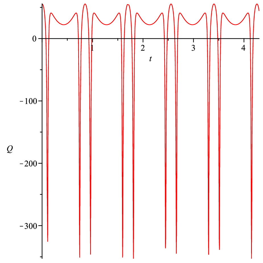
The absence of big bang singularities in the present models are very easy to understand when one observes the Bohmian quantum potential eq. (16), for those models. We have computed eq. (16), for several values of negative , all possible values of and many different wavefunctions constructed as linear combinations of the energy eigenfunctions and corresponding time sectors. The calculations were made over the Bohmian trajectories of . It means that reduces to a function that depends only on . We have found the same qualitative behavior of , in all those cases. Initially, at , there is a potential barrier () that prevents the value of ever to go through zero. Then, the barrier becomes a well for a brief moment and again a new barrier appears (). After a while, turns into a well for a brief moment and then another barrier identical to appears. After that , periodically, repeats itself. is different from . exists for a longer period and is shorter than . One may interpret the potential shape in the following way. Initially, at , starts to grow from its minimum value different from zero, first rapidly, and then its velocity starts to decrease until it goes to zero, at the maximum value of . Then, starts to decrease, first slowly, and then its velocity starts to increase until reaches its minimum value different form zero. There, its velocity changes sign and starts to grow once more, as described above. This dynamics is represented in , initially, by , then the first well, then and finally the well just after . Then the movement of repeats itself periodically. These models have no big bang singularities because and its periodic repetitions prevent ever to go through zero. In order to exemplify this behavior we show, in Figure 2, the Bohmian quantum potential eq. (16), for the model with , . The wavefunction was obtained by the linear combination of two energy eigenfunctions and corresponding time sectors with eigenvalues and given in Table 1. For a better visualization of ’s behavior, we choose a small time interval in Figure 2. For a clearer understand of ’s behavior we have plotted, in Figure 3, the Bohmian trajectory of for the model with the same conditions described in Figure 2, during the same time interval of Figure 2 and initial condition at . This initial condition was obtained from the calculation of the expected value of , for the same model and the same linear combination of energy eigenstates and corresponding time sectors of the model described in Figure 2.
Acknowledgements. G. Oliveira-Neto, E. V. Corrêa Silva and G. A. Monerat (Researchers of CNPq, Brazil) thank CNPq and FAPERJ for partial financial support. We thank the opportunity to use the Laboratory for Advanced Computation (LCA) of the Department of Mathematics, Physics and Computation, FAT/UERJ, where part of this work was prepared.
References
- [1] B. S. DeWitt, Phys. Rev. D 160 (1967) 1113.
- [2] D. Bohm and B. J. Hiley, The undivided universe: an ontological interpretation of quantum theory, Routledge, London, 1993;
- [3] P. R. Holland, The quantum theory of motion: an account of the de Broglie-Bohm interpretation of quantum mechanics, Cambridge University Press, Cambridge, 1993.
- [4] F. G. Alvarenga, J. C. Fabris, N. A. Lemos, G. A. Monerat, Gen. Rel. Grav. 34 (2002) 651.
- [5] N. A. Lemos, G. A. Monerat, Gen. Rel. Grav. 35 (2003) 423.
- [6] J. Acacio de Barros and N. Pinto-Neto, Int. J. Mod. Phys. D 7 (1998) 201;
- [7] J. Acacio de Barros, N. Pinto-Neto and M. A. Sagioro-Leal, Phys. Lett. A 241 (1998) 229.
- [8] G. Oliveira-Neto, E. V. Corrêa Silva, N. A. Lemos, G. A. Monerat, Phys. Lett. A 373 (2009) 2012.
- [9] P. Pedram, M. Mirzaei, S. Jalalzadeh, S. S. Gousheh. Gen. Rel. Grav. 40 (2008) 16631681.
- [10] N. A. Lemos, F. G. Alvarenga, Gen. Rel. Grav. 31 (1999).
- [11] N. A. Lemos, J. Math. Phys. 37 (1996) 1449.
- [12] M. J. Gotay and J. Demaret, Phys. Rev. D 28 (1983) 2402.
- [13] N. Pinto-Neto, Proceedings of the VIII Brazilian School of Cosmology and Gravitation II, ed. M. Novello (1999).
- [14] V. G. lapchinskii and V. A. Rubakov, Theor. Math. Phys. 33 (1977) 1076.
- [15] Edésio M. Barboza Jr. and Nivaldo A. Lemos, Gen. Rel. Grav. (2006) 38 16091622.
- [16] B. F. Schutz, Phys. Rev. D 2 (1970) 2762; Phys. Rev. D 4 (1971) 3559.
- [17] Joseph Polchinski, in: L. Baulieu, J. de Boer, B. Pioline and E. Rabinovici (eds.), String theory: From gauge interactions to cosmology, Springer, Berlin, 2005, pp. 229-253
- [18] Alexander Vilenkin, in: H. Suzuki, J. Yokoyama, Y. Suto and K. Sato (eds.), Inflating Horizons of Particle Astrophysics and Cosmology, Universal Academy Press, Tokyo, 2006.
- [19] E. V. Corrêa Silva, G. A. Monerat, G. Oliveira-Neto, C. Neves and L. G. Ferreira Filho, Phys. Rev. D 80 (2009) 047302.
- [20] J. V. José and E. J. Saletan, Classical Dynamics: A Contemporary Approach, Cambridge University Press, Cambridge, 1998.