The history of beta decay began in 1896 with the discovery of radioactivity by Henri Becquerel. In the years 1899 and 1900 he identified $\beta$ radiation as one component of radioactivity, and demonstrated that $\beta$ rays are composed of electrons, comparing it with the properties of cathode rays. Unfortunately the rapidity with which $\beta$ rays were identified after their discovery did not lead to an equally rapid interpretation of the $\beta$ decay process. At that moment physicists knew that certain substances have the same chemical properties but different radioactive properties (isotopes). As experiments improved, the interpretations of the $\beta$ decay phenomenon became more and more confusing. Chadwick in 1914, using a magnetic spectrometer, discovered the continuous spectrum of the $\beta$ particles. Thus it was known that the electron spectra had monoenergetic lines and a continuous component, in contrast with alpha and gamma ray spectra, which were known to consist of monoenergetic lines only. Chadwick further demonstrated that the majority of events were part of the continuous component, the rest being monoenergetic electrons from electron conversion. The interpretation of the continuous electron spectrum was the main subject of the discussion. In 1914 Rutherford thought that the $\beta$ electrons were all emitted from the nucleus with the same energy, but lost different fractions of this energy in collisions with the surrounding atoms, depending on the source thickness. But the main point was made by Lise Meitner in 1922. She realized that a quantized nucleus could not emit electrons of continuous energy. The known features of $\alpha$ and $\gamma$ spectra were correctly interpreted as due to transitions of nuclei from one quantum state to another. Thus the continuous electron spectrum was a unique feature of $\beta$ decay.
The measurement of the mass of different isotopes was determinant to conclude the existence of a neutral mass inside the nucleus, but the common thought was that this neutrality was due to the neutralization of the proton with an atomic electron which falls into the nucleus. Nevertheless, the uncertainty principle only allows electrons inside the nucleus with an energy greater than $\sim$100 MeV¹¹ 1 This rough calculation was made considering the size of the nucleus $\sim$ 1 [fm], but now we know that the size of the nucleus is $\sim$ 6 [fm], and considering this value the uncertainty principle allows electrons inside the nucleus with energies $\sim$ 16 MeV (the maximum energy of the electron $\beta$ continuous spectrum is around 10 MeV). And consequently the electrons could not exist ”a priori” in the nucleus.

In 1927 a crucial experiment was performed by Ellis and Wooster, in which they measured the total energy released in the disintegration of a ²¹⁰Bi source inside a calorimeter thick enough to stop all the emitted electrons. The endpoint of the electron $\beta$ spectrum was known to be $E_{o}$=1.05 MeV, and the mean energy, $\bar{E}$, of the $\beta$ electrons was known to be 390 keV. The calorimeter should have measured a total energy of 1.05 MeV if Rutherford’s reasoning was correct. In fact they observed $\bar{E}$ = 344 $\pm$ 34 keV, which corresponded very well with the mean energy of the emitted electrons. The experiment was repeated in Berlin with an improved calorimeter by Meitner and Orthman in 1930 and the result was $\bar{E}$=337 $\pm$ 20 keV. These results were conclusive, Rutherford was wrong, but difficult to interpret at the time.
In $\beta$ decay not only was energy apparently not conserved, but the momentum and angular momentum were not conserved either. Pauli in 1931 proposed the idea of a very penetrating neutral particle of very small mass and spin $1/2$ being emitted simultaneously with the electron. Thus, the problem of the conservation of energy, momentum and spin was solved. This proposal was made before Chadwick’s discovery in 1932 of the neutral elementary particle, the neutron, and it was Fermi who named Pauli’s particle as the neutrino. In this way the process of emission of electrons from the nucleus was explained and scientifically accepted.
In 1934 Irene and Frédéric Joliot-Curie observed the emission of positive electrons (later called positrons) in radioactive decay. And in 1938 Alvarez observed the electron capture from the nearest electronic orbits.
This brings us to our present knowledge of $\beta$-decay which we can describe as,

• 1.-

  $\beta^{-}$ decay: In this process a neutron ($n$) of the nucleus is converted into a proton ($p$) due to the week interaction, emitting an electron ($e^{-}$) and an antineutrino ($\bar{\nu}$).

  $$n\rightarrow p+e^{-}+\bar{\nu}$$

  (1.1)

• 2.-

  $\beta^{+}$ decay: In this process a proton ($p$) of the nucleus is converted into a neutron ($n$) due to the week interaction emitting a positron ($e^{+}$) and a neutrino ($\nu$).

  $$p\rightarrow n+e^{+}+\nu$$

  (1.2)

• 3.-

  Electron Capture: In the electron capture process, also called inverse $\beta^{+}$ decay, an electron ($e^{-}$) from the inner shell of the atom is captured by the nucleus, converting a proton ($p$) into a neutron ($n$) and emitting a neutrino ($\nu$).

  $$p+e^{-}\rightarrow n+\nu$$

  (1.3)

In 1934 Fermi developed a theory of the $\beta$ decay process to include the neutrino, presumed to be massless²² 2 Today we think that the neutrino has some mass, although very small as well as chargeless, dealing with the calculation of the transition probability of the process of $\beta$ decay. This cannot be done starting from any other theory. A complete new force had to be introduced to explain the $\beta$ transition which converts a neutron into a proton (or viceversa) and at the same time produces an electron (positron) and a antineutrino (neutrino). Such a force was introduced by Fermi, using the analogy with the electromagnetism.
The transition probability in the $\beta$ decay process can be given in terms of the first-order, time-dependent perturbation theory, later called the Fermi Golden Rule,

$$\lambda=\frac{2\pi}{\hbar}|\langle f|H_{\beta}|i\rangle|^{2}\rho_{f}$$

(1.4)

where $\langle f|H_{\beta}|i\rangle$ is the matrix element of the beta interaction $H_{\beta}$ between the initial state $|i\rangle$ and the final state $|f\rangle$ of the complete system (nucleus and other relevant light particles), and $\rho_{f}$ is the density of final states in the final system. The final state of the system is specified by the electron and neutrino momenta and energies, $(p_{e},E_{e})$ and $(p_{\nu},E_{\nu})$, with $E_{\nu}=cp_{\nu}$. If $E_{f}$ denotes the energy in the final system, we have

$$\rho_{f}dE_{f}=V^{2}\frac{p^{2}_{e}dp_{e}d\Omega_{e}}{(2\pi\hbar)^{3}}\frac{p^{2}_{\nu}dp_{\nu}d\Omega_{\nu}}{(2\pi\hbar)^{3}}$$

(1.5)

where $V$ is a spherical volume in the momentum space and

$$E_{f}=E_{e}+E_{\nu}=E_{e}+p_{\nu}c$$

(1.6)

Without fixing the directions of the momenta, we have

$$\rho_{f}=V^{2}(4\pi)^{2}\frac{p^{2}_{e}dp_{e}p^{2}_{\nu}}{(2\pi\hbar)^{6}}\frac{dp_{\nu}}{dE_{f}}$$

(1.7)

Fermi did not know the mathematical form of the interaction $H_{\beta}$ in $\beta$ decay. But in considering all possible forms consistent with special relativity, he showed that $H_{\beta}$ could be replaced by an operator $O_{x}$ which could, mathematically, take the form of a vector($V$), scalar($S$), pseudoscalar($P$), axial vector ($A$) or tensor ($T$). So, for beta decay,

$$\langle f|H_{\beta}|i\rangle=W_{fi}=\sum_{x}g_{x}\int d\vec{r}\left[\Phi^{*}_{f}\psi^{*}_{e}\psi^{*}_{\nu}\right]O_{x}\Phi_{i}$$

(1.8)

where $\Phi_{f}$, $\psi_{e}$ and $\psi_{\nu}$ are the final wave functions of the nucleus after the decay, the electron and the neutrino. The value of $g_{x}$ determines the strength of the interaction. The electron and neutrino are treated like free-particles, thus their wave functions have the form,

$$\psi_{e}(\vec{r})=\frac{1}{\sqrt{V}}e^{i\vec{p_{e}}\cdot\vec{r}/\hbar},\qquad\psi_{\nu}(\vec{r})=\frac{1}{\sqrt{V}}e^{i\vec{p_{\nu}}\cdot\vec{r}/\hbar}$$

(1.9)

If we expand the exponentials, using the fact that over the nuclear volume $pr\ll 1$, we have the allowed approximation. If we replace the electron and neutrino wave functions in eq.1.8 and use the allowed approximation, the matrix element is now $gM_{fi}=g\int d\vec{r}\Phi^{*}_{f}O\Phi_{i}$, so the decay rate is

$$\lambda=\frac{g^{2}}{2\pi^{3}\hbar^{7}}\int\frac{dp_{\nu}}{dE_{f}}p^{2}_{e}p^{2}_{\nu}|M_{fi}|^{2}dp_{e}$$

(1.10)

for a fixed $E_{e}$ the term $\frac{dp_{\nu}}{dE_{f}}=1/c$. On the other hand, if we define $Q$ as the total decay energy, the momentum of the neutrino is $p_{\nu}=(Q-T_{e})/c$. The decay rate is now

$$\lambda=\frac{g^{2}}{2\pi^{3}\hbar^{7}c^{3}}\int dp|M_{fi}|^{2}p^{2}(Q-T_{e})^{2}$$

(1.11)

but here we are not taking into account the interaction between the beta particle and the Coulomb field in the daugther nucleus. In order to take this effect into account an additional factor was added to the decay rate, $F(Z^{\prime},p)$ where $Z^{\prime}$ is the atomic number of the daughter nucleus. The total decay rate is now

$$\lambda=\frac{g^{2}|M_{fi}|^{2}}{2\pi^{3}\hbar^{7}c^{3}}\int^{p_{max}}_{0}p^{2}(Q-T_{e})^{2}F(Z^{\prime},p)dp.$$

(1.12)

This integral only depends on $Z^{\prime}$ and the maximum electron energy $E_{0}$, and it is represented as

$$f(Z^{\prime},E_{0})=\frac{1}{m^{5}_{e}c^{7}}\int^{p_{max}}_{0}p^{2}(Q-T_{e})^{2}F(Z^{\prime},p)dp$$

(1.13)

where the constants have been included to make $f$ dimensionless. This function is known as the Fermi integral and it is tabulated for values of $Z^{\prime}$ and $E_{0}$.
As $\lambda=ln(2)/T_{1/2}$, we have,

$$fT_{1/2}=\frac{2ln(2)\pi^{3}\hbar^{7}}{g^{2}m^{5}_{e}c^{4}|M_{fi}|^{2}}$$

(1.14)

The equation 1.14 gaves the comparative halflife or ft value.

In the allowed approximation the electron and the neutrino are created at the origin ($r=0$). As the orbital angular momentum is zero($l=0$), the only change in the angular momentum is due to the spins of the electron ($s_{e}=1/2$) and neutrino ($s_{\nu}=1/2$). If the two spins are antiparallel ($S=0$), there is no change in the nuclear spin: $\Delta I=|I_{i}-I_{f}|=0$. This is known as Fermi Decay ($F$). If the electron and neutrino spins are parallel ($S=1$), they carry away an angular momentum of $1$, therefore $I_{i}$ and $I_{f}$ must be coupled through a vector of length 1: $\vec{I}_{i}=\vec{I}_{f}+\vec{1}$. This is possible for $\Delta I=0$ or $1$ (except for $I_{i}=0$ and $I_{f}=0$, when only Fermi transitions can contribute). This is known as Gamow-Teller Decay ($GT$). They are governed by different operators which we will called $O_{F}$ and $O_{GT}$ in an obvious notation.

The matrix elements of $F$ and $GT$ decays must be written separately. The matrix elements for Fermi Decay, following equation 1.8, is

$$M_{fi}=M_{F}=g_{V}\int d\vec{r}\Phi^{*}_{f}O_{F}\Phi_{i}$$

(1.15)

and for the Gamow-Teller Decay

$$M_{fi}=M_{GT}=g_{A}\int d\vec{r}\Phi^{*}_{f}O_{GT}\Phi_{i}$$

(1.16)

The Fermi operator is expressed as $O_{F}=\sum^{A}_{i=1}\tau_{\pm}(i)$ where $\tau_{+}$ ($\tau_{-}$) is the isospin ladder operator converting the proton(neutron) wavefunction into a neutron(proton) wavefunction. For Gamow-Teller decay the corresponding operator is $O_{GT}=\sum^{A}_{i=1}\vec{\sigma}(i)\tau_{\pm}(i)$ where $\vec{\sigma}(i)$ are the Pauli matrices, which also act on the ith nucleon. Now we can rewrite the equation 1.14 in terms of the Fermi and Gamow-Teller matrix elements.

$$fT_{1/2}=\frac{K}{|M_{F}|^{2}+\frac{g^{2}_{A}}{g^{2}_{V}}|M_{GT}|^{2}}=\frac{K}{B(F)+\frac{g^{2}_{A}}{g^{2}_{V}}B(GT)},\quad\textrm{where}\quad K=\frac{2ln(2)\pi^{3}\hbar^{7}}{g^{2}_{V}m^{5}_{e}c^{4}}$$

(1.17)

and $B(F)$ and $B(GT)$ are the dimensionless Fermi and Gamow-Teller strengths.

The charge symmetry and charge Independence of the nuclear interaction and the almost equality of the masses of the neutron and the proton strongly suggest that they are the same particle (the nucleon) in two different charge states. [1, 2, 3]
In analogy with the reorientation of the two degenerate states of the electron spin under the effect of a magnetic field in the real space, a nucleon under the influence of a electromagnetic field, can differentiate the two degenerate isospin states or charge states in the charge space or isospin space. A nucleon with third isospin component $T_{z}=-1/2$ (down) is defined as a proton, and a nucleon with third isospin component $T_{z}=+1/2$ (up) is defined as a neutron.³³ 3 The isospin assignment for a neutron and a proton, which is adopted here, is conventional in nuclear physics and has the advantage that the heavy nuclei with large neutron excess have their isospin aligned in the direction of the positive z axis in the isospin space. In elementary particle physics, the inverse sign convertion is usually adopted.[3]. The isospin obeys the usual rules for angular momentum vectors. The isospin vector $\tau$ has a length of $\sqrt{\tau(\tau+1)}\hbar$ and with 3-axis projections $\tau_{z}=m_{\tau}\hbar$.
For a system of several nucleons, the isospin follows the same coupling rules as the ordinary angular momentum vectors. The 3-axis component of the total isospin vector, $T_{z}$, is the sum of the 3-axis components of the individual nucleons, and for any nucleus

$$T_{Z}=\sum^{A}_{i=1}t_{z}(i)=\frac{1}{2}(N-Z)$$

(1.18)

expressed in units of $\hbar$.[5]

The assumption that the attractive nuclear force is independent of the charge of the interacting nucleons is one of the bases of our understanding of nuclear physics. This assumption hides a simple and elegant symmetry: The isospin symmetry (or charge symmetry).

In the isospin approach, all nucleons must have an isospin $t=1/2$ differentiating protons and neutrons by its projections. The use of isospin gives us a simple way to classify nuclei according to the third component of their isospin.
A state in a nucleus with $N=Z$ corresponds to a particular configuration of neutrons and protons. If an identical state cannot be constructed in the neighbouring nucleus with $N-1$ neutrons and $Z+1$ protons by exchanging a neutron by a proton then the original state must have isospin $T=0$, because it can only be constructed in a nucleus with $N-Z=0$, which has projection $T_{z}=0$. The $N=Z$ nucleus can also have a state with $T=1$, which, because $T_{z}\pm 1$ is also allowed, can be constructed identically in the $N\pm 1$, $Z\mp 1$ systems(see Figure 1.1). [4]

The $T_{z}=+1$ to $T_{z}=0$ transitions could be studied in charge exchange (CE) reactions ($(p,n)$-type [6],[7] or $(^{3}$He$,t)$-type[8],[9]), and the $T_{z}=-1$ to $T_{z}=0$ transitions can be investigated in $\beta$ decay experiments as shown in Figure 1.1. Such studies have only been performed in detail so far for light nuclei, such as the $A=26$ system (²⁶Mg, ²⁶Al and ²⁶Si)[10]. One major constraint for these studies in light nuclei is that $\beta$ decays can access only a few low-lying states due to the restriction imposed by the $Q_{\beta}$-window. Among the $T=-1\rightarrow 0$ candidates, the analogue transitions in the $fp$ shell nuclei are well suited to an accurate study of isospin symmetry. The reason is that due to relatively large $Q_{EC}$ values, the $\beta$ decay studies should allow $B(GT)$ measurements up to high excitation energies in the daughter nuclei.

The ⁵⁴Fe target located in a gas cell was bombarded with a primary ³He beam at 45 MeV coming from the CYCLONE110 cyclotron. Several radioactive nuclei were created in this reaction but since we have an on-line mass separator we are only concerned about the production, selection and mass separation of the ⁵⁴Ni and ⁵⁴Co nuclei.

The decay of ⁵⁴Ni is difficult to study because its production is always overwhelmed by the direct production of its daugther nucleus ⁵⁴Co. Indeed the calculated production cross section for the ⁵⁴Ni has a maximum of 30 $\mu$barn at an energy of 45 MeV for the ³He beam. At the same energy the ⁵⁴Co has a production cross section of 5 $m$barn (166 times bigger)[19].

The ⁵⁴Fe(³He,2np)⁵⁴Co and ⁵⁴Fe(³He,3n)⁵⁴Ni reactions are produced in the gas cell. A laser beam selectively ionizes either Ni or Co atoms. The resonant ions are extracted and accelerated by a DC electrical field and directed to the mass separator which separates the single-charged, A=54 mass ions by $A/q$. In the following we give a detailed explanation of the different components of the LISOL device.

In the $\beta$ decay of ⁵⁴Ni we expect to have three type of radiation: betas, neutrinos and gammas. It is difficult to detect the neutrinos but we can make a sensitive setup to detect $\beta$ radiation and $\gamma$-rays. For the $\gamma$-ray detection we used two MINIBALL Ge cluster detectors and for the $\beta$ particles we used plastic detectors. Three $1.3$ mm thick plastic $\beta$ detectors were placed around the implantation point (tape ending, see Figure 2.4). In most of the cases the $\beta$ particle only deposits part of its energy in the thin plastic. These detectors were used to determine if a $\beta$ particle passed through the detector or not. No energy was registered.

Two MINIBALL clusters were located as close as possible to two of the scintillators. The MINIBALL detector is a cluster of three hyper-pure germanium crystals, each of them six-fold segmented. The crystals and the capsules are tapered in a hexagonal shape to fit three of them side-by-side in a single cryostat. A positive high voltage is applied to a lithium-diffused centre contact, which penetrates deep inside the germanium. Six boron-implanted contacts on the surface of each crystal constitute the segmented outer contacts. An incident $\gamma$-ray interacts with the Ge crystal and transfers its energy either totally (photoelectric effect) or partially (Compton or pair creation) to an electron, this electron loses its kinetic energy, creating a number of electron-hole pairs. Within the fully depleted region of germanium between the contacts, the charge created goes to the corresponding electrode. Thus, the electrons go to the centre contact (core signal), and the holes go to the outer contacts (segment signal) (See Figure 2.5) .
The charge collected on the crystal contacts is integrated by charge-sensitive resistor feedback preamplifiers, developed and produced by the Institute of Nuclear Physics in Cologne, a member institute of the MINIBALL Collaboration.[18]

After the mass separation, the ions are implanted on a thin 1.25 cm wide aluminium-coated mylar tape. The thickness of the tape is chosen to stop the beam completely. The tape rewinding system is located below the detectors. The tape from one of the two coils goes up, intercepts the beam path, goes up again and turning fully down, comes again below the detector level and finally ends in the second coil. The part of the tape where the ions are implanted is moved down to a safe distance away from the detectors, to avoid the background produced by the activity of long-lived ions close to stability. The whole tape system is kept in the same vacuum as the beam transport line. There are three thin mylar windows in the chamber around the implantation area to reduce the attenuation of the radiation of interest.
A schematic picture of the detector setup and the tape system is shown in Figure 2.6.

The preamplified signals are provided to the analogue inputs of the DGF-4C modules. The DGF (Digital Gamma Finder) can measure the amplitude and the shape of the incoming pulses simultaneously. The energy information is extracted directly from the preamplified signal height and the time information is obtained from a built-in high-precision internal clock after the event validation.
In our detector system we have 21 signals from each MINIBALL $\gamma$ detector (3 signals from the cores and 18 segments) and another 3 signals from the three plastic scintillator $\beta$ detectors. Since an incident $\gamma$ ray is registered by the core and some of the segments of the same crystal, there is a time correlation between the signals from one crystal. Further on there should be no segment signal unless there is a signal from the corresponding crystal core. For these reasons, the DGF modules are split into trigger groups, in which each group represents one crystal and the core channel is the main trigger of the group. The logic signals from the $\beta$ detectors are provided to one DFG module and their inputs are set independently. To estimate the total acquisition live time, a pulser signal feeds one channel of a DGF module. This value is represented by the ratio between the registered pulser signals to the number of pulses provided by the pulser.

A new C++ software code has been created by Oleg Ivanov and Dieter Pauwels from Katholieke Universiteit Leuven, to read and analyze the data acquired by the detection setup. The object oriented ROOT package developed at CERN is used for building the output histograms. While building the singles spectra is a simple procedure, the $\beta$-n$\gamma$ and n$\gamma$ coincidences, where n represents the number of $\gamma$-detectors (crystals), are based on the event time stamps. These coincidences are stored in ROOT trees for further analysis[18].

The resolution check for the MINIBALL detectors was performed with a ⁶⁰Co source. The measured resolutions for all MINIBALL crystals at 1332 keV are shown in the next table for the ”Heidelberg” and ”Leuven” clusters.

Heidl.A	3.4 keV	LeuvenA	3.3 keV
Heidl.B	2.7 keV	LeuvenB	3.1 keV
Heidl.C	2.8 keV	LeuvenC	3.0 keV

The $\gamma$ efficiency calibrations (See Figure 3.2) were performed after the experiment with a ¹⁵²Eu positioned on the tape at the point of implantation. The activity of the source at the time of the experiment was 23.87 kBq.

The same ¹⁵²Eu source was used before the experiment, for the on-line analysis energy calibration. Afterwards, for off-line analysis, an internal energy calibration was performed using the ⁵⁴Co^m gamma cascade present in our experiment for each ROOT file created after more or less each one hour of running time.

With all the calibrated spectra, several control measurements were performed before and during the experiment in order to optimize the production and mass separation of ⁵⁴Ni and ⁵⁴Co^g,m.

• 1.-

  Laser tuning on Co: To optimize the selectivity of Co ions by laser resonance in the gas cell, we looked at the ratio in intensity of 411 keV and 511 keV $\gamma$-ray lines from the decay of ⁵⁴Co^g,m in the singles and $\beta-\gamma$ coincidence spectra with a fixed mass 54 in the mass separator. The cyclotron current and the tape steps were also fixed. Short measurements of 100 seconds with and without laser resonance were made.

• 2.-

  Mass tuning: Once the selectivity was optimized, we proceeded to tune the mass selection on the separator with laser resonance on Co looking at the integral of the 411 keV line in the singles and $\beta-\gamma$ spectra, taking short measurements of 100 seconds.

• 3.-

  Gas Buffer Pressure and Cyclotron Current: With the mass optimized and with laser resonance on Co, the optimal gas buffer pressure was found looking again at the 411 keV line in the singles and $\beta-\gamma$ spectra, taking short measurements of 100 seconds. After this the cyclotron current was tuned following the same procedure as described above.

• 4.-

  Tape Step and Implantation-Decay Macrocycle: In the previous ⁵⁴Ni $\beta$ decay experiment developed by I.Reusen et al.[17],[19] the measured halflife was 106(12) ms. Consequently, a proper 400 ms and 600 ms implantation-decay macrocycle was chosen for this experiment. The tape was moved one step every six macrocycles in order to minimize the time lost during the tape rewinding.

In the following table the starting settings are summarized.

Mass	53.94
Cyclotron Current	4.0 $\mu$A
Gas Buffer Pressure	760 mbar
ID Macrocycle	400 ms / 600 ms
Tape Movement Period	6 Macrocycles

These settings were checked and, if necessary, modified during the experiment in order to increase the selectivity and mass separation of the ion of interest.

After seven days of experiment, the data acquisition time with laser resonance on Ni was 115 hours. The time used for the laser resonance on Co was 16 hours. The total number of counts in the 411 keV ⁵⁴Co^m decay radiation in the laser on Ni total spectrum was 94,817 while the number of counts in the 411 keV peak in the laser on Co total spectrum was 46,903. Finally, the settings adjustment time was 2.5 hours. Singles and $\beta$-$\gamma$ coincidence spectra were constructed in ROOT trees to facilitate the on line analysis. These pre-processed data were also used for the off-line analysis.
In general the data analysis was done with the $\beta$-$\gamma$ coincidence spectra. As we are interested also in the high energy GT excited states, a veto condition (see Figure 3.3) was imposed in order to reduce the background produced by the penetration of the $\beta$ particle into the MINIBALL crystal. The main idea is that if a $\beta$ particle is detected in a plastic detector, the gamma detector situated behind it is not used. In Figure 3.4 we see the difference between the spectrum with the no-veto condition, which has 5,984 counts in the 937 keV peak and with the veto condition, which has 3,886 counts in the 937 keV peak. Although the upper spectrum has higher statistics, the lower one has a better peak-to-total ratio.

Figures 3.5 and 3.6 represent the total $\gamma$ spectra of mass 54 activity with the laser set on resonace for Ni and Co respectively. Both of them were constructed with the no-$\beta$ penetration veto condition. In the laser on Ni spectrum we can observe the 937 keV $\gamma$ line known in the decay of ⁵⁴Ni. The gamma cascade lines 411 keV, 1130 keV and 1408 keV from the ⁵⁴Co^m decay and the 922 keV sum peak (411 keV + 511 keV) are also present. Another peak is observed in the spectra at 683 keV with a measured halflife of $\sim$ 180 ms, but it is not yet identified. See also Figure 3.7 for the low energy part of the spectra. In the laser set on Co spectrum, the same cascade lines and sum peaks are present but not the 937 keV line.

From the previous experiment[17] we know that the ⁵⁴Ni halflife is 106(12) ms, thus if we take into account the macrobeam structure (400 ms of implantation and 600 ms of decay) and the microbeam structure due to the mass separator time behaviour during the implantation, we can model our Implantation Decay Curve, simply by solving the decay differential equations.

$$\frac{d}{dt}N_{1}(t)=P(t)-\lambda_{1}N_{1}(t)\qquad N_{1}(0)=0$$

(3.1)

$$\frac{d}{dt}N_{2}(t)=\lambda_{1}N_{1}(t)-\lambda_{2}N_{2}(t)\qquad N_{2}(0)=0$$

(3.2)

$$P(t)=\sum_{i=1}^{4}a(H(t-50(2i-1))-H(t-100i))$$

$$H(t-b)=\left\{\begin{array}[]{ll}0&\textrm{if $t<b$}\\ 1&\textrm{if $t\leq b$}\end{array}\right.$$

where $N_{1}$ is the ⁵⁴Ni activity, $N_{2}$ is the ⁵⁴Co activity, $\lambda_{1}$ and $\lambda_{2}$ are the respective decay constants and $P(t)$ is the implantation rate of ⁵⁴Ni, taking into account the microbeam structure. $H(t)$ is the Heaviside step function and $a$ is the constant implantation rate when $P(t)\neq 0$.
Solving the differential equation with the initial conditions for $N_{1}(t)$ and $N_{2}(t)$ using Maple10^tm, we obtain the implantation decay curves of ⁵⁴Ni and ⁵⁴Co (Fig.3.8).

On the other hand, from our experiment we obtain a $\beta$ gated $\gamma$ spectrum, thus we can reproduce the ID curve looking at the time evolution of the 937 keV peak during one macrocycle. The time difference between each of the spectra (50 ms) was chosen in order to be consistent with the time behaviour of the mass separator. This way we can find the halflife value of ⁵⁴Ni by looking at the time behaviour of the integral of the 937 keV $\gamma$ line.

The analysis of the halflife of ⁵⁴Ni can be deduced from the time behaviour of the area of the 937 keV peak after background substraction in the laser on Ni $\gamma$ spectrum.

As a first approach to obtaining the halflife we integrated a fitted Gaussian with 937 keV centroid, subtracting a linear background close to the Gaussian (centroid $\pm$ twice FWHM region). Figure 3.9 shows the evolution of the 937 keV peak during an ID macrocycle. The last four spectra corresponding to the last 200 ms show that the intensity of the 937 keV line became of the same order as the background. For that reason, the last four points were neglected in the fit of the micro implantation-decay curve (see Figure 3.10). In this case, the error obtained in fitting a Gaussian for each experimental point in Fig.3.10 is calculated with the ROOT minimization package MINUIT. ¹¹ 1 MINUIT calculates an error matrix with the parameters. This error matrix is the inverse of the second derivative matrix of the best parameter values (the function minimum) and the diagonal elements of the error matrix are the square roots of the individual parameter errors, including the effect of correlation with the other parameters. The value obtained for the halflife of the ⁵⁴Ni in this case was T_1/2= 114.9 $\pm$ 6.0 ms. The halflife error was obtained from the fit to the implantation-decay curve including the micro structure, again using the ROOT minimization package MINUIT.

Another attempt to deduce the halflife as precisely as possible was made by fitting two Gaussians, one on the 922 keV sum peak and the other on the 937 peak, the second one with a fixed width (see Figure 3.11). The value of the width was taken from the width of the Gaussian fit in the total spectra. The so called long background (linear background taken from 800 keV to 1100 keV) was used to subtract the background in the region of interest, in order to reduce background fluctuations in the vicinity of the 937 peak. A reduced error bar is obtained with this method in comparison with the first attempt. Again, the error obtained by fitting a double gaussian for each experimental point in Fig.3.10 is calculated with the ROOT minimization package MINUIT. However it is also clear from this fit that the last points do not behave in the expected way and should therefore be ignored in the $T_{1/2}$ fit. This tells us that due to the lack of statistics (peak indistinguishable from the background) at the end of the macrocycle, we can eliminate those points in order to fit a proper curve to determine the halflife. The value of the halflife of the ⁵⁴Ni for this case was T_1/2= 113.8 $\pm$ 4.4 ms. The halflife error was obtained from the fit of the implantation-decay curve including the micro structure using again the ROOT minimization package MINUIT.

A third method to measure the halflife of the ⁵⁴Ni was to integrate directly the 937 keV peak and subtract the long linear background (See Figure 3.13). The error bar is a statistical error obtained from the integration of the 937 keV peak. If we again neglect the last 200 ms of the macrocycle, the halflife value was T_1/2= 113.7 $\pm$ 4.6 ms(See Figure 3.14). The halflife error was obtained from the fit of the implantation-decay curve including the micro structure using again the ROOT minimization package MINUIT.

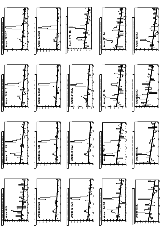
In spite of the good agreement shown between these three different halflife analyses, it is worth mentioning that the estrange behaviour at the end of the ID curve clearly suggested that some correlation existed between the range of the background chosen and the halflife obtained. Indeed in the 937 keV region, in addition to the 922 keV sum peak, there is the Compton edge of the 1130 keV $\gamma$ peak. This made it very difficult to decide if the background that we were subtracting was the correct one or not.

A semi-empirical model for the $\gamma$-ray response of the germanium detectors [20] was used to estimate the correct shape of the background for background subtraction under the 937 keV line. In this analysis was include:

• a.-

  The full energy peak: A Gaussian distribution with variance $B_{1}^{2}$ and normalization parameter $A_{1}$

  $$f_{1}(E_{0},E)=\frac{A_{1}}{\sqrt{2\pi}B_{1}}exp\left(\frac{(E-E_{0})^{2}}{2B_{1}^{2}}\right)$$

  (3.3)

• b.-

  The Flat continuum: A constant function when folded with a Gaussian function gives an expression of the form

  $$f_{2}(E_{0},E)=A_{2}\textrm{\emph{erfc}}\left(\frac{(E-E_{0})}{\sqrt{2}B_{1}}\right)$$

  (3.4)

• c.-

  The single Compton scattering: The expression for the energy deposited in a single Compton scattering is well documented in textbooks. In order to account for the roll-off at the Compton edge that is observed in experimental spectra, Y.Jin et al. determine the electron energy function with a complementary error function,

  $$f_{3}(E_{0},E)=A_{3}\left[\left(\frac{E_{0}}{E_{0}-E}\right)+\left(\frac{E_{0}-E}{E_{0}}\right)-1+\cos^{2}\theta\right]\textrm{\emph{erfc}}\left(\frac{(E-B_{2})}{\sqrt{2}B_{3}}\right),\quad E\leq E_{c}$$

  $$f_{3}(E_{0},E)=0,\qquad E>E_{c}$$

  (3.5)

  $$\cos\theta=1+\left(\frac{m_{0}c^{2}}{E_{0}}\right)+\left(\frac{m_{0}c^{2}}{E_{0}-E}\right)$$

  and

  $$E_{c}=\frac{E_{0}}{\left[1+\frac{m_{0}c^{2}}{2E_{0}}\right]}$$

• d.-

  Multiple Compton scattering Y.Jin et al. have derived expressions for the energy deposition due to two and three Compton scatters. The derivation assumed that the spatial distribution of once-scattered and twice-scattered photons within the detector, are uniform. They give a set of equations for the energy deposition function for the double Compton scattering $f_{4}(E_{0},E)$

  $$f_{4}(E_{0},E)=0,\qquad\alpha^{\prime\prime}>\alpha$$

  $$f_{4}(E_{0},E)=A_{4}\int_{\alpha^{\prime\prime}}^{\alpha}H(\alpha,\alpha^{\prime})H(\alpha^{\prime},\alpha^{\prime\prime})d\alpha^{\prime},\qquad\frac{\alpha}{1+2\alpha}<\alpha^{\prime\prime}<\alpha$$

  $$f_{4}(E_{0},E)=A_{4}\int_{\frac{\alpha}{1+2\alpha}}^{\frac{\alpha^{\prime\prime}}{1-2\alpha^{\prime\prime}}}H(\alpha,\alpha^{\prime})H(\alpha^{\prime},\alpha^{\prime\prime})d\alpha^{\prime},\qquad\frac{\alpha}{1+4\alpha}<\alpha^{\prime\prime}<\frac{\alpha}{1+2\alpha}$$

  $$f_{4}(E_{0},E)=0,\qquad 0<\alpha^{\prime\prime}<\frac{\alpha}{1+4\alpha}$$

  (3.6)

  where

  $$H(\alpha,\alpha^{\prime})=\frac{\alpha^{\prime}}{\alpha^{3}}+\left(\frac{1}{\alpha}+\frac{2}{\alpha^{2}}-\frac{2}{\alpha^{3}}\right)\left(\frac{1}{\alpha^{\prime}}\right)+\frac{1}{\alpha^{2}\alpha^{\prime 2}}+\frac{2}{\alpha^{3}}+\frac{1}{\alpha^{4}},$$

  and

  $$\alpha=\frac{E_{0}}{m_{0}c^{2}},\qquad\alpha^{\prime}=\frac{E^{\prime}}{m_{0}c^{2}},\qquad\alpha^{\prime\prime}=\frac{E^{\prime\prime}}{m_{0}c^{2}},\qquad E^{\prime\prime}=E_{0}-E.$$

  The energy deposition function $f_{5}(E_{0},E)$ for the triple Compton scattering is given by the following set of equation

  $$f_{5}(E_{0},E)=0,\qquad\alpha^{\prime\prime}>\alpha,$$

  $$f_{5}(E_{0},E)=A_{5}\int_{\alpha^{\prime\prime}}^{\alpha}\int_{\alpha^{\prime\prime}}^{\beta}H(\alpha,\beta)H(\beta,\gamma)H(\gamma,\alpha^{\prime\prime})d\gamma d\beta,\qquad\frac{\alpha}{1+2\alpha}<\alpha^{\prime\prime}<\alpha$$

  	$\displaystyle f_{5}(E_{0},E)=A_{5}\int_{\frac{\alpha}{1+2\alpha}}^{\frac{\alpha^{\prime\prime}}{1-2\alpha^{\prime\prime}}}\int_{\alpha}^{\beta}H(\alpha,\beta)H(\beta,\gamma)H(\gamma,\alpha^{\prime\prime})d\gamma d\beta\quad+$
  			$\displaystyle A_{5}\int_{\frac{\alpha^{\prime\prime}}{1-2\alpha^{\prime\prime}}}^{\alpha}\int_{\frac{\beta}{1+2\beta}}^{\frac{\alpha^{\prime\prime}}{1-2\alpha^{\prime\prime}}}H(\alpha,\beta)H(\beta,\gamma)H(\gamma,\alpha^{\prime\prime})d\gamma d\beta,\qquad\frac{\alpha}{1+4\alpha}<\alpha^{\prime\prime}<\frac{\alpha}{1+2\alpha}$

  $$f_{5}(E_{0},E)=A_{5}\int_{\frac{\alpha}{1+2\alpha}}^{\frac{\alpha^{\prime\prime}}{1-4\alpha^{\prime\prime}}}\int_{\frac{\beta}{1+2\beta}}^{\frac{\alpha^{\prime\prime}}{1-2\alpha^{\prime\prime}}}H(\alpha,\beta)H(\beta,\gamma)H(\gamma,\alpha^{\prime\prime})d\gamma d\beta,\quad\frac{\alpha}{1+6\alpha}<\alpha^{\prime\prime}<\frac{\alpha}{1+4\alpha}$$

  $$f_{8}(E_{0},E)=0,\qquad 0<\alpha^{\prime\prime}<\frac{\alpha}{1+6\alpha}$$

  (3.7)

  All these integrals can be solved analytically.

In this same paper, Jin gives the parameters $A_{i}$ and $B_{i}$ as a function of the energy.

$$A_{1}=-0.937680+0.203032\times 10^{1}E_{0}^{-0.2}-0.892372E_{0}^{-0.4}\qquad,$$

$$A_{2}=-0.110826\times 10^{-1}+\frac{0.911437\times 10^{-1}}{\sqrt{E_{0}}}\qquad,$$

$$A_{3}=0.721355\times 10^{-2}+\frac{0.185895}{E_{0}^{2}}\qquad,$$

$$A_{4}=-0.775913\times 10^{1}+0.204322\times 10^{2}E_{0}^{0.1}-0.124189\times 10^{2}E_{0}^{0.2}\qquad,$$

$$A_{5}=-0.343254\times 10^{-2}+0.213600\times 10^{-1}E_{0}-0.882892\times 10^{-3}E_{0}^{2}\qquad,$$

$$B_{2}=-0.156849+0.965065E_{0}\qquad\textrm{, and}$$

$$B_{3}=0.443463\times 10^{-1}+0.1697733\times 10^{-1}E_{0}\qquad.$$

As a first attempt to fit the calculated background we used the 1407 keV peak. This peak was chosen because its Compton edge can be easily distinguished in the ⁵⁴Ni and ⁵⁴Co spectra. The integrals in (3.7) and (3.8), were solved analytically with MAPLE10^tm and its solutions with the full energy peak, single Compton scattering and the flat continuum are presented in Figure 3.15.

In Figure 3.16 is shown the ⁵⁴Co total spectrum with the calculated background. A correction factor was applied to this calculated background in order to equal the amplitude of the full energy peak of 1407 keV with the measured spectrum. A good agreement between the theoretical background and the real data is presented, but no further analysis has been done up to the time of writing.

In Figure 3.17 we present the energy spectra obtained in the ⁵⁴Fe(³He,t)⁵⁴Co charge exchange reaction [21]. In addition to the $0^{+}\rightarrow 0^{+}$ Fermi transition and the first $0^{+}\rightarrow 1^{+}$ Gamow-Teller transition, other high energy states are populated in the reaction. Because in the $\beta$ decay case we have a $Q$-value window up to $\sim$8.8 MeV we also expected to populate some of these states. Because of the expected drop in $\beta$-branching due to the $f$ factor and the drop of the $\gamma$-ray detection efficiency at high $\gamma$-energies, we expect to see the 3375 keV peak more easily than the other higher lying states. We therefore searched for the 3375 keV peak.

In the Figure 3.18 the 3375 keV region is plotted, but no $\gamma$ lines are distinguishable from the background.

With the three values obtained from the behaviour of the 937 keV $\gamma$ line the value of the ⁵⁴Ni halflife is calculated as the weighted mean ²² 2 This is a preliminar estimation of the halflife, and certainly is not the right way to do it because this three values are not calculated from independent measurements. which value is $T_{1/2}=114\pm 3$ ms. With this value we can estimate the absolute Gamow-Teller strength, using equation 1.24.

$$\frac{1}{T_{1/2}}=\frac{B(F)(1-\delta_{c})}{K\sigma^{F}}\left(\sigma^{F}f_{F}+\frac{\lambda^{2}}{R^{2}}\sum_{i=GT}\sigma_{i}^{GT}f_{i}\right)$$

where $T_{1/2}=0.114(3)$ s is the measured halflife, $B(F)=2$ is the $|N-Z|$ value, $(1-\delta_{c})=0.995$ is the Coulomb correction factor, $\sigma^{F}=4905\pm 245$ is the number of counts in the $0^{+}\rightarrow 0^{+}$ transition in the charge exchange reaction (see Figure 3.17 ), $f_{F}=22107\pm 746$ and $\sum_{i=GT}\sigma_{i}^{GT}f_{i}=(130.9\pm 8.1)\times 10^{6}$, $K=6144.4\pm 1.6$ where the $f$ values are given by the $f$-function calculation, and $\lambda^{2}=1.603\pm 0.007$. With these values we can calculate the $R^{2}$ value which is related to the $B(GT)$ as is shown in Eq. (1.24).

	$\displaystyle\frac{1}{0.114\pm 0.003}=\frac{2\times 0.995}{(6144.4\pm 1.6)\times(4905\pm 245)}\quad\times$
			$\displaystyle\times\left[(1.0844\pm 0.0908)\times 10^{8}+\frac{1.603\pm 0.007}{R^{2}}\times(130.9\pm 8.1)\times 10^{6}\right]$

$$R^{2}=8.56\pm 0.73$$

$$B(GT)_{(T_{1/2}=114\pm 3)}=0.48\pm 0.08\quad.$$

(3.8)

The calculated absolute Gamow-Teller strength is $B(GT)=0.48\pm 0.08$.

References

- [1] H.H. Heckman & P.W. Starring, ”Nuclear Physics and the Fundamental Particles”. Holt, Rinehart and Winston, INC. (1963).
- [2] R.R. Roy & B.P. Nigam, ”Nuclear Physics: Theory and Experiment”. John Wiley & Sons, INC. (1967).
- [3] A. Bohr & B.R Mottelson, ”Nuclear Structure. Vol 1: Single Particle Motion”. World Scientific Publishing Co.Pte.Ltd. 2nd Edtion (1998).
- [4] D.D. Warner, M.A. Bentley and P. Van Isacker, Nature Physics 2 311-318 (2006).
- [5] K.S. Krane, ”Introductory Nuclear Physics”. John Wiley & Sons, INC. 2nd Edition (1988).
- [6] T.N. Taddeucci et al., Nucl. Phys. A469 125-172 (1987).
- [7] E. Hagberg et al., Phys. Rev. Lett. 73 396-399 (1994).
- [8] Y. Fujita et al., Nucl. Phys A687 311c-320c (2001).
- [9] R.G.T. Zegers et al., Phys.Rev. C 74 024309 (2006).
- [10] Y.Fujita et al., Phys.Rev. C 67 064312 (2003).
- [11] C.D. Goodman et al., Phys. Rev. Lett 44 1755 (1980).
- [12] Y. Fujita. Journal of Physics: Conference Series 20 107-112 (2005).
- [13] Y. Fujita. Journal of Physics: Conference Series 49 29-34 (2006).
- [14] Y. Kudryavtsev et al., Nucl. Inst. and Meth. B 114 350-365 (1996).
- [15] Y. Kudryavtsev et al., Nucl. Inst. and Meth. B 179 412-435 (2001).
- [16] P. Van den Berg et al., Nucl. Inst. and Meth. B 126 194-197 (1997).
- [17] I. Reusen et al., Phys.Rev. C 59 2416-2421 (1999)
- [18] O. Ivanov. PhD thesis. Katholieke Universiteit Leuven.
- [19] I. Reusen. PhD thesis. Katholieke Universiteit Leuven, 1999.
- [20] Y.Jin, R.P. Gardner and Verghese, Nucl. Inst. and Meth. in Phyics Research A 242 416-426 (1986)
- [21] Y. Fujita et al. Private communication.