Foreground Maps in WMAP frequency bands

Tuhin Ghosh ^†^†thanks: E-mail: tuhin@iucaa.ernet.in Affiliation: IUCAA, Post Bag 4, Ganeshkhind, Pune-411007, India Affiliation: APC 10, rue Alice Domon et Leonie Duquet, 75205 Paris Cedex 13, France Jacques Delabrouille ^†^†thanks: E-mail: delabrouille@apc.univ-paris7.fr Affiliation: APC 10, rue Alice Domon et Leonie Duquet, 75205 Paris Cedex 13, France Mathieu Remazeilles ^†^†thanks: E-mail: remazeil@apc.univ-paris7.fr Affiliation: APC 10, rue Alice Domon et Leonie Duquet, 75205 Paris Cedex 13, France Jean-François Cardoso ^†^†thanks: E-mail: cardoso@tsi.enst.fr Affiliation: APC 10, rue Alice Domon et Leonie Duquet, 75205 Paris Cedex 13, France Tarun Souradeep ^†^†thanks: E-mail: tarun@iucaa.ernet.in Affiliation: IUCAA, Post Bag 4, Ganeshkhind, Pune-411007, India

Accepted Received

Abstract

This paper provides full sky maps of foreground emission in all WMAP channels, with very low residual contamination from the Cosmic Microwave Background (CMB) anisotropies and controlled level of instrumental noise. Foreground maps are obtained by subtraction of a properly filtered CMB map, obtained from linear combinations of needlet-based representations of all WMAP observations and of a 100–micron map. The error in the reconstructed foreground maps on large scales is significantly lower than the original error due to CMB contamination, while remaining of the order of the original WMAP noise on small scales. The level of the noise is estimated, which permits to implement local filters for maximising the local signal to noise ratio. An example of such filtering, which reduces the small scale noise using latitude dependent filters is implemented. This enhances significantly the contrast of galactic emission, in particular on intermediate angular scales and at intermediate galactic latitude. The clean WMAP foreground maps can be used to study the galactic interstellar medium, in particular for the highest frequency channels for which the proper subtraction of CMB contamination is mandatory. The foregrounds maps can be downloaded from a dedicated web site.

Keywords:

Needlets, Galaxy maps, Point sources, Diffuse emissions

1 Introduction

The WMAP space mission, launched by NASA in 2001, has been primarily designed to measure the anisotropies of the Cosmic Microwave Background (CMB) emitted when the universe became transparent, at an age of about 380,000 yr. The interpretation of these observations in the context of the standard hot Big-Bang model has constrained the main parameters of the model with great accuracy (Komatsu et al., 2009).

In addition to the primordial CMB, WMAP detectors are sensitive to foreground astrophysical emission: diffuse emission from the galactic interstellar medium (ISM), emission from compact extragalactic sources (such as radiogalaxies and AGN and, to lesser extent, thermal Sunyaev-Zel’dovich (SZ) emission from clusters of galaxies). Hence, maps observed by WMAP contain each a mixture of emissions from different astrophysical processes.

The analysis of the observed maps for deriving a CMB power spectrum, in temperature or polarization, involves some kind of foreground cleaning, followed by masking the regions of the sky most contaminated by foregrounds, and estimation of the angular spectrum $C_{\ell}^{\rm CMB}$ of the CMB on the masked sky. There exist several ways to deal with the incomplete sky coverage for power spectrum estimation (Hivon et al., 2002; Efstathiou, 2004; Faÿ et al., 2008). Little is lost in terms of power spectrum estimation accuracy by masking a small fraction of sky (the accuracy is typically reduced by a factor $f_{\rm sky}$ equal to the fraction of the sky kept for the analysis). Proper estimation of the contamination (biasing) of the power spectrum by noise or residual foreground emission permits to correct for the contribution of both kinds of contaminants on the power spectrum of the CMB map.

Where to give up foreground cleaning and resort, instead, to masking, is an interesting (and debated) issue. To be on the safe side, conservative masking is typically used for estimating the CMB power spectrum. However, low–level foreground emission often remains in the masked sky (see, e.g., Patanchon et al. (2005); Leach et al. (2008)).

Foreground emissions of various astrophysical origins, however, are of much scientific interest themselves. Scientific investigation of foregrounds cannot resort to masking regions contaminated by CMB, the latter being present everywhere on the sky. In recent observations, such as those of WMAP, the CMB is stronger than the noise on a large range of angular scales, in all regions of the sky. The analysis of foreground emission in WMAP data, hence, requires subtraction of the CMB contaminant (which is the main source of error) while keeping contamination by instrumental noise as small as possible. Obtaining such clean foreground intensity maps from WMAP data is the objective of the present paper.

2 Method

Standard methods for component separation (see Delabrouille & Cardoso (2007) for a review) often assume that the data are well represented by noisy linear mixtures of well-defined components, e.g. CMB, SZ, thermal dust, synchrotron, etc. Most methods used in the CMB context such as Wiener filtering (Bouchet & Gispert, 1999; Tegmark & Efstathiou, 1996), Maximum Entropy Methods (Hobson et al., 1998), Independent Component Analysis (ICA) methods of different types (Maino et al., 2002; Delabrouille et al., 2003) explicitly represent sky emission as a superposition of emissions, the properties of which are parametrised in some way. In reality, matter emits via a great variety of distinct processes, and there is no obvious way of separating the total emission into distinct components. It is probably fair to argue that there is, for instance, no natural preferred option between distinguishing components via their emission process (e.g. synchrotron vs. free-free) or via their place of origin (the ISM of our galaxy vs. the ISM of other galaxies). Similarly, dust emission arises from a variety of forms of matter (from molecules to large dust grains), and from several emission processes (thermal greybody emission, electric dipole emission from rotating dust grains…). Whether to distinguish thermal dust from spinning dust as two separate components, or instead distinguish between warm and cold dust, for instance, is a matter of taste. One can also consider dust emission as being all emission from all matter that is not ionised – the appropriate modeling depends on the scientific question addressed. The obvious exception to this is the CMB, which is distinct both by its origin (the last scattering surface) and its spectral emission law. If, however, the WMAP experiment was sensitive enough for kinetic SZ effect (which has the same spectral emission law as primordial CMB fluctuations) to be above the noise level, the question of whether to distinguish the two would become relevant as well.

2.1 The model

Given that complexity of foreground emission, and the relative lack of spectral resolution in WMAP data (only 5 channels, for many different emission processes), one must extend the way to parametrise foreground emission. Extensions of the Spectral Matching ICA (SMICA) method (Delabrouille et al., 2003) to allow more flexible models of foreground emission are discussed by Cardoso et al. (2008a); Cardoso et al. (2008b).

In the present analysis, we adopt the extreme point of view in which we choose to distinguish between three contributions to the WMAP maps only: CMB, foregrounds (dominated by the emission of the galactic ISM), and noise. The task we address, then, is to produce the best possible maps of foregrounds with minimal contamination from CMB and noise. Further analysis of the foreground component into different emissions of interest (whether by origin, or by emission process) is not the aim of this paper.

The temperature map at a given frequency channel of WMAP is given by

x^{i}(p)=\int b^{i}(p.p^{\prime})\left[s(p^{\prime})+f^{i}(p^{\prime})\right]\,dp^{\prime}+n^{i}(p),

(1)

where $i$ indexes the WMAP frequency bands, and runs from 1 to 5. $s(p)$ and $f^{i}(p)$ are respectively the CMB and foreground components, and $n^{i}(p)$ is the instrumental noise in the given frequency band. Here, $b^{i}(p.p^{\prime})$ is the beam of the observed map for the $i^{th}$ frequency band (assumed to be symmetric, but not necessarily Gaussian). The direction on the sky (or pixel of a pixelized map) is indexed by $p$ . Equation 1 can be written in harmonic space as:

x^{i}_{\ell m}=b_{l}^{i}\left[s_{\ell m}+f^{i}_{\ell m}\right]+n^{i}_{\ell m}

(2)

Our objective is to estimate in the best possible way the foreground emission $\int b^{i}(p.p^{\prime})f^{i}(p^{\prime})dp^{\prime}$ (or equivalently $b_{l}^{i}f^{i}_{\ell m}$ ) in each WMAP channel. Once stated in that way, the problem becomes quite well posed. The CMB emission has the particular feature that it is completely uncorrelated from the other two, and that its emission law is known (it is the derivative of a blackbody with respect to temperature, at temperature $T_{\rm CMB}=2.725\,$ K). The instrumental noise is well characterised. It is well approximated as uncorrelated from channel to channel. Its level is known with excellent accuracy, and it is known to dominate at high angular frequencies (high $\ell$ ).

The foreground component is everything else, i.e. everything that comes from the sky (rather than from the instrument) and is not CMB. We set no other constraint on this foreground component, i.e. we assume no particular parametrization of it.

2.2 Separation strategy

We propose to extract the foreground component by subtracting an estimate of the CMB from the total maps, and then post-processing the remaining set of CMB–cleaned WMAP data to get maps of foreground emission. The effectiveness of this procedure is discussed in section 4 and appendix A.

Considering the minimal assumptions made about the foregrounds, it is quite natural to use the so-called Internal Linear Combination method (ILC) to extract a CMB map, to be subtracted from WMAP data to produce CMB-free foreground maps. The ILC is a multifrequency linear filter which uses a linear combination of the input data. It minimizes the variance of the reconstructed CMB map over domains of observation as, e.g, regions of the sky, or domains in harmonic space, or domains in needlet space.

The strategy for obtaining foreground maps is thus the following:

•

estimate a CMB map using an ILC;
•

subtract that CMB from the WMAP frequency maps (at proper resolution);
•

filter to maximize the signal to noise ratio in each of the foreground maps.

2.3 The needlet ILC

Considering the variability of the statistical properties of foregrounds and noise both in pixel space and in harmonic space, the optimisation of the separation calls for localisation of the filter in both spaces. That can be achieved with needlets, which are a special type of wavelets on the sphere (Narcowich et al., 2006; Marinucci et al., 2008; Guilloux et al., 2009). A needlet–based ILC is well suited to our component separation problem, as localisation in direct space (in addition to localisation in harmonic space) permits better reconstruction of the CMB in the vicinity of the galactic plane, i.e. a region of major interest for foreground science. For the present analysis, we use for CMB subtraction the WMAP 5-year needlet-based ILC map (NILC map) obtained by Delabrouille et al. (2009), and displayed in figure 1. Other options were considered, as for instance the harmonic ILC map derived in Saha et al. (2006); Saha et al. (2008), as has been done in Ghosh et al. (2009). The NILC map has been chosen here because it reconstructs best the CMB in regions where foregrounds are significant.

Refer to caption — Figure 1: The clean CMB map extracted using internal linear combination in needlet space, used for CMB subtraction in the present analysis

It can be written as:

\hat{s}_{\ell m}=b_{\ell}^{W}s_{\ell m}+\delta_{\ell m}

(3)

where $\delta_{\ell m}$ is the CMB reconstruction error and where the beam is denoted $b_{\ell}^{W}$ , corresponding to the resolution of channel W. The angular spectrum of that map is

\mathrm{E}|\hat{s}_{\ell m}|^{2}=B_{\ell}^{W}C_{\ell}^{\mathrm{CMB}}+N_{\ell}^{\rm ILC}

(4)

with $N_{\ell}^{\rm ILC}=\mathrm{E}(\delta_{\ell m})^{2}$ and $B_{\ell}^{W}=(b_{l}^{W})^{2}$ .

2.4 Channel–dependent CMB subtraction

In our present application, the objective is to subtract the CMB in each channel, without adding significant additional noise (and, obviously, without adding more noise than we subtract CMB). In each channel, the total emission observed (eq. 2) comprises a CMB contribution $b_{\ell}^{i}s_{\ell m}$ . We subtract from each observation map $x_{\ell m}^{i}$ a rebeamed, rescaled version of the needlet ILC map, that is, the foreground map $f_{\ell m}^{i}$ at the resolution of channel $i$ is estimated by

\hat{f}_{\ell m}^{i}=x_{\ell m}^{i}-\alpha_{\ell}\frac{b_{\ell}^{i}}{b_{\ell}^{W}}\hat{s}_{\ell m}

(5)

where the coefficient $\alpha_{\ell}$ can be chosen to minimise the reconstruction error, denoted $\varepsilon_{\ell m}^{i}$ , and defined by:

\hat{f}_{\ell m}^{i}=b_{l}^{i}f_{\ell m}^{i}+\varepsilon_{\ell m}^{i}.

(6)

Indeed, eqs (2), (3) and (5) show that

\varepsilon_{\ell m}^{i}=(1-\alpha_{\ell})b_{\ell}^{i}s_{\ell m}-\alpha_{\ell}\frac{b_{\ell}^{i}}{b_{\ell}^{W}}\delta_{\ell m}+n^{i}_{\ell m}

(7)

Neglecting the correlation between $\delta_{\ell m}$ and $n_{\ell m}^{i}$ , one gets

\mathrm{E}(\varepsilon_{\ell m}^{i})^{2}=(1-\alpha_{\ell})^{2}B_{\ell}^{i}C_{\ell}^{\rm CMB}+\alpha_{\ell}^{2}\frac{B_{\ell}^{i}}{B_{\ell}^{W}}N_{\ell}^{\rm ILC}+\mathrm{E}(n_{\ell m}^{i})^{2}

(8)

where $B_{\ell}^{i}=(b_{\ell}^{i})^{2}$ . The mean square error $\mathrm{E}(\varepsilon_{\ell m}^{i})^{2}$ is easily found to be minimal for

\alpha_{\ell}=\frac{C_{\ell}^{\rm CMB}}{C_{\ell}^{\rm CMB}+N_{\ell}^{\rm ILC}/B_{\ell}^{W}}.

(9)

This is exactly the signal to signal-plus-noise ratio in (4), that is, the prescription for Wiener filtering. Therefore, the variance of the foreground map in channel $i$ (at the resolution of the channel), is minimal if we subtract the Wiener-filtered version of the needlet ILC map.

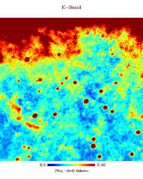
CMB subtraction according to (5) yields our primary foreground map in WMAP channel $i$ , at the resolution of the considered WMAP channel. The map contains essentially foreground emission and noise from channel $i$ , and additional error originating from imperfect CMB subtraction. This additional error is discussed in more detail in section 4.3. Figure 2 illustrates for one of the WMAP channels (here, the K band at 23 GHz), on a patch centered at modest galactic latitude (latitude -30 degree and longitude 70 degree), the separation of the original observation into CMB and foregrounds. The effect of CMB subtraction is clearly visible when comparing the original map (top left) to the map after CMB has been subtracted (bottom left). Most of the large to intermediate scale fluctuations due to the presence of CMB have been removed, which permits to identify clearly compact sources and structures of the galactic emission.

2.5 Latitude-dependent filtering

After CMB subtraction, the estimated foreground map $\hat{f}_{\ell m}^{i}$ still contains significant noise, which dominates on small scales. This is clearly visible in the bottom left panel of figure 2. That map is obtained, by construction, at the resolution of the original input map but we still have extra degrees of freedom: adjusting the beam or, equivalently, multiplying the harmonic modes by some filter $w_{\ell}^{i}$ , one obtains a new estimate $\tilde{f}_{\ell m}^{i}$ of the foreground map as:

\tilde{f}_{\ell m}^{i}=w_{\ell}^{i}\hat{f}_{\ell m}^{i}

The filter can be adjusted to minimize the total variance

\sum_{\ell}\sum_{m=-\ell}^{\ell}\mathrm{E}\left|\tilde{f}_{\ell m}^{i}-b_{\ell}^{i}f_{\ell m}^{i}\right|^{2},

and it is well known that, in the ideal case where both the foreground map of interest $f_{\ell m}^{i}$ and the contamination term $\varepsilon_{\ell m}^{i}$ are stationary, the best filter is the Wiener filter:

w_{\ell}^{i}=\frac{B_{l}^{i}C_{\ell}^{\rm FG}}{B_{l}^{i}C_{\ell}^{\rm FG}+E_{\ell}}

where $E_{\ell}$ is the variance of the reconstruction error $\varepsilon_{\ell m}^{i}$ .

However, we are not facing a stationary situation. As galactic foregrounds are strongly concentrated in the galactic plane, the filtering should better depend on the location on the sky. It is not immediately clear what would be the best strategy for such a localized filtering, especially if there is need not only to provide the best map but also to characterize it. As a reasonable compromise between efficiency and simplicity, we approximate the foreground emission as following a plane parallel slab model. We then apply a filter for each zone of galactic latitude. As discussed in the next section, we also constrain the total response after filtering to have a Gaussian shape, i.e. we find the Gaussian beam which fits best the harmonic response $w_{\ell}^{i}b_{\ell}^{i}$ resulting from the instrumental beam and the Wiener filter. In that way, the variation of the beam across the sky can be described simply by a latitude dependent (actually: depending only on the latitude zone) Gaussian beam. The improvement of the quality of the derived foreground map after filtering is clearly visible in figure 2, where the bottom right panel displays the foreground map after the filtering. Details of the implementation are given in the next section.

3 Practical implementation

3.1 CMB subtraction

For each WMAP channel, we start from the Wiener filtered Needlet ILC CMB from Delabrouille et al. (2009) which includes the $\alpha_{\ell}$ ratio of eq. 9. The resolution of the map is changed in harmonic space, by multiplication of each $a_{\ell m}$ by the ratio $b_{\ell}^{i}/b_{\ell}^{W}$ . The resulting CMB map is subtracted from the observation in channel $i$ . Note that because of the Wiener filter applied on the CMB map, the equivalent resolution of this CMB map is not that of channel $i$ .

The foreground map obtained in a given channel by subtraction of the CMB contains foregrounds, noise, and a residual (the difference between the CMB estimate and the true CMB at the resolution of the given channel). The residual contains some noise from all channels, some residual CMB, and a small amount of foregrounds. This residual, however, is well below the foreground emission on large scales and orders of magnitude below the noise of the considered WMAP band on small scales. This is illustrated, for four of the WMAP channels, in figure 3, which displays the power spectra of the WMAP observations after CMB subtraction, as compared to the original CMB contamination, to contamination by noise, and to the residual due to improper CMB subtraction. In all channels, the process of CMB subtraction reduces by two orders of magnitude the total contamination power on the largest scales. For the V channel, a significant reduction of the total contamination is achieved up to $\ell$ larger than 500.

3.2 Latitude zones

The sky is divided into 7 latitude zones, selected using multiplicative masks. Each mask is defined as follows:

$\displaystyle M(\theta,\phi)$	$\displaystyle=1\ \$	$\displaystyle\text{for}\ \theta_{0}<\|\theta\|<\theta_{1}$
	$\displaystyle=\cos^{2}\left(\frac{\pi}{2}\times\frac{\theta_{0}-\|\theta\|}{\Delta\theta}\right)\ \$	$\displaystyle\text{for}\ \theta_{0}-{\Delta\theta}\leq\|\theta\|<\theta_{0}$
	$\displaystyle=\cos^{2}\left(\frac{\pi}{2}\times\frac{\|\theta\|-\theta_{1}}{\Delta\theta}\right)\ \$	$\displaystyle\text{for}\ \theta_{1}<\|\theta\|<\theta_{1}+\Delta\theta$
	$\displaystyle=0\ \$	elsewhere.

Here $\Delta\theta$ is the width of transition regions of the mask (regions in which its value decreases smoothly from 1 to 0). The latitudes $\theta_{0}$ and $\theta_{1}$ are the lower and upper limits of the region where the mask value is 1. Note that each region is symmetric with respect to the galactic plane. Smooth transitions in the masks for the different latitude bands simply permit to avoid edge effects in the masked maps, mitigating mode mixing in the calculation of power spectra. Limits for the zones (i.e. values for $\theta_{0}$ and $\theta_{1}$ ) used in this analysis are 0, 5, 10, 20, 30, 45, 60 and 90 degrees, with transitions of $\Delta\theta=5^{\circ}$ . The width of the regions selected in this way increases with increasing galactic latitude, which is required for accurate estimation of the Wiener filter (see below).

3.3 Latitude-dependent Wiener filter

For each channel, for each latitude band, we compute the power spectrum $C_{\ell}^{\rm OUT}$ of the masked noisy foreground map. For each $\ell$ , the total power comprises a contribution $F_{\ell}$ from the foregrounds $b_{\ell}^{i}f_{\ell m}^{i}$ at the resolution of channel $i$ (i.e. the signal of interest) and a contribution $E_{\ell}$ from the reconstruction error $\varepsilon_{\ell m}^{i}$ . In this case, the Wiener filter can be approximated as:

w_{\ell}=\frac{C_{\ell}^{\rm OUT}-E_{\ell}}{C_{\ell}^{\rm OUT}}.

(10)

See section 4.3 for the estimation of $E_{\ell}$ . The Wiener filter as defined by equation 10 is applied independently in each WMAP channel.

The effective beam after Wiener filtering becomes $w_{\ell}b_{\ell}^{i}$ . That is the beam which minimizes the variance of the error of the reconstructed foreground map, for channel $i$ , in the latitude band defined by the mask corresponding to the zone considered. In fact, such a Wiener filter can be computed locally for any region of interest, not only for latitude bands, which are used here mainly for illustrative purposes.

3.4 Gaussian beam approximation

As discussed above, it is not very convenient to construct a final foreground map in which the beam varies rapidly over the sky. For simplicity, it may also be desirable to work with effective Gaussian beams, in which case the beam is fully defined by a single number: its full width at half maximum (FWHM). The beam response in harmonic space then is:

b_{\ell}^{\rm gauss}=\text{exp}\left(-\frac{\ell(\ell+1)\sigma^{2}}{2}\right)

where $\sigma$ is related to the FWHM of the Gaussian beam by the relation $\sigma=\theta_{\rm FWHM}/\sqrt{(8\times\log 2)}$ .

For each of our seven selected regions then, we determine the Gaussian beam which best matches the theoretical optimal effective beam due to the effect of both the instrumental beam and the Wiener filter. We derive a FWHM which varies smoothly in latitude bands of 5 degree width by interpolating the FWHM derived using the broader latitude bands described in 3.2 above. The corresponding FWHM, for all WMAP channels and all latitudes in 5 degree steps, is plotted in figure 5.

Note that while our choice results from a trade-off between optimality and convenience, it is somewhat arbitrary. We could, for instance, have decided to work with more complex symmetrical beam shapes or different zones. We stress, however, that no information is lost in that process since one can always change back the response in harmonic space (and change the effective beam) by multiplication of $a_{\ell m}$ coefficients by the appropriate response ratio. The FWHM plotted in figure 5 are just indicative of the scales where noise starts to dominate over the foregrounds, as a function of channel and galactic latitude.

3.5 Construction of the filtered maps

After having determined, for each frequency channel, the resolution at which the foreground map should be reconstructed as a function of galactic latitude, a filtered final map for each WMAP channel is obtained in the following way. Starting from the original WMAP observations and after CMB removal, we make 18 different maps, one at the appropriate resolution for a 5–degree wide latitude band. The final map for that channel is obtained by picking, for each pixel of the final map, the corresponding pixel in the one of the 18 maps which is at the resolution matching the latitude band of the pixel at hand. Hence, the resolution of the filtered map varies in steps over the sky, with a change in resolution at all multiples of $5^{\circ}$ .

4 Discussion

4.1 Multi-frequency analyses

As seen in figure 5, the Gaussian beam which maximises the signal to noise ratio of the foreground map in a given channel depends both on galactic latitude and on the channel.

Further analysis of these foreground maps, however, involves measuring spectral indices in selected regions or the spectral energy distribution of compact sources, i.e. ratios between flux at different frequencies. Such post-analyses require maps at the same resolution.

For specific, localised analyses, using several WMAP channels, original CMB-cleaned maps can easily be re-beamed for better matching of the resolution with the local S/N ratio. Figure 5 provides a helpful tool for choosing the resolution of the analysis. To take a specific example, for investigations involving all channels at 25 degrees latitude, one should pick a resolution somewhere between 30 and 50 arc-minutes, as the curves giving the appropriate resolution, for each channel, in that latitude zone, give numbers between 30 and 50.

4.2 Faint foregrounds?

Although the original claim in the present work is the construction of maps of all foregrounds, it should be noted that the final maps are appropriate only for the scientific analysis of foregrounds whose contribution to the observed emission is larger than the WMAP noise (but can be smaller than the CMB), i.e. of galactic foregrounds and strong point sources.

The reason is as follows. The subtracted CMB has been obtained by an ILC method, which finds locally linear combinations which minimise the total variance of the CMB reconstruction error. When subdominant foregrounds are present, it is more favourable to the ILC to let weak foregrounds leak in the CMB map and reduce the instrumental noise, than the opposite. For instance, Sunyaev Zel’dovich effects are too weak to play a role in the adjustment of the linear combinations used for CMB reconstruction in WMAP data. The same is true for a weak background of point sources. Hence, the ILC is not optimised to reject these foregrounds, which thus are not preserved in the final foreground maps produced with our processing. A search for SZ signals in WMAP data has been performed by Melin et al. (2010) using a method appropriate for this particular signal, the multifrequency matched filter (Herranz et al., 2002; Melin et al., 2006).

4.3 Noise levels

The ‘noise’ in our foreground maps (from all sources of error) in the map for channel $i$ (at the resolution defined by the beam $b_{\ell}^{i}$ ) comes from four main terms:

1.

noise $n^{i}$ from the relevant WMAP channel;
2.

noise $\sum w_{j}n^{j}$ from ‘internal linear combinations’ of WMAP channels, present in the CMB map subtracted from each WMAP observation;
3.

foregrounds leaking in the needlet ILC estimate of the CMB;
4.

CMB residuals after subtraction of the estimated CMB.

An exact characterisation of the total error is not completely possible in the absence of a reliable model of the foregrounds, which is needed to estimate the amount of foreground emission leaking in the estimated CMB. It is possible, however, to give an estimate of the total ‘noise’ power spectrum, $E_{\ell}$ .

4.3.1 Noise power spectrum estimate

An estimate is obtained by considering that all terms are independent so that the total power of the error is the sum of the powers of all contributions.

The first term is simply the noise power $N_{\ell}^{i}$ of the WMAP $i^{\rm\it{th}}$ channel, the level of which is provided with the release of WMAP data.

The second term is estimated by Monte-Carlo simulations of the WMAP noise by Delabrouille et al. (2009). Noise maps and power spectra released are available on a dedicated web page¹¹ 1 http://www.apc.univ-paris7.fr/APC/Recherche/Adamis/cmb_wmap-en.php. They should be corrected from the effect of the Wiener filtering and rebeaming. This is done by multiplying each mode, in harmonic space, by:

r_{\ell}=\frac{b_{\ell}^{i}\,w_{\ell}}{(b_{\ell}^{\rm NILC})^{2}}

(11)

where $w_{\ell}$ is the effective beam of the Wiener-filtered needlet ILC CMB map, $b_{\ell}^{i}$ is the beam of the foreground map, and $b_{\ell}^{\rm NILC}$ the beam of the NILC map (coinciding, for $\ell<1000$ , with that of the W channel. The power $N_{\ell}^{\rm CMB}$ of the error from this term is:

N_{\ell}^{\rm CMB}=r_{\ell}^{2}N_{\ell}^{\rm ILC}

(12)

where $N_{\ell}^{\rm ILC}$ is the noise level, per harmonic mode, available with the needlet ILC CMB map.

The third term is unknown. On the vast majority of the sky where foregrounds are weak, it is negligible. Where foregrounds are strong, it is always a small fraction of the input foregrounds. It is therefore neglected in our noise estimate.

The fourth term comprises contributions from two effects: a) residual CMB from the difference between the beam of the WMAP channel considered and the effective beam of the subtracted CMB, which can be computed straightforwardly; b) CMB modes cancelled by the ILC because of empirical correlation with the foregrounds and noise (see appendix and figure 6 and of Delabrouille et al. (2009)).

Appendix B gives a detailed calculation of all noise terms. The power $E_{\ell}$ of the sum of all contributions (total error) is given by the expression:

E_{\ell}\simeq N_{\ell}^{i}+r_{\ell}^{2}N_{\ell}^{\rm ILC}+\\ \left[\left(b_{\ell}^{i}\left(1-\alpha_{\ell}\right)\right)^{2}+0.04\,b_{\ell}^{i}\left(1-\alpha_{\ell}\right)b_{\ell}^{W}r_{\ell}\right]C_{\ell}^{\rm CMB}

(13)

where $C_{\ell}^{\rm CMB}$ is the CMB power spectrum (which can be taken to be the WMAP best fit model, for instance). The last term is the total contribution from CMB subtraction error. The first term in the brackets comes from effect a) above, and the second term is a correction originating from the 2% CMB power loss due to the ILC bias.

Figure 7 shows the decomposition of the total noise into three main terms: noise from WMAP in channel Ka, noise from the NILC map, and residual CMB improperly subtracted.

Figure 8 displays the power spectra of all foreground maps, and power spectra of the noise term in all of them.

4.3.2 Noise power spectrum upper limit

The two first terms (i) and (ii) (arising from WMAP instrumental noise) are correlated because the instrumental noise in the estimated CMB contains a part of the noise on the channel of interest. An upper limit to the total error is obtained by assuming that the correlation is perfect between $n^{i}$ and $\sum w_{j}n^{j}$ , which is the case when channel $i$ dominates with a negative coefficient in the ILC (negative, because the ILC is subtracted from channel $i$ to get the foreground map).

Hence, we can assume the following upper limit for $E_{\ell}$ :

E_{\ell}\leq\left[\left(N_{\ell}^{i}\right)^{\frac{1}{2}}+r_{\ell}\left(N_{\ell}^{\rm ILC}\right)^{\frac{1}{2}}\right]^{2}+\\ \left[\left(b_{\ell}^{i}\left(1-\alpha_{\ell}\right)\right)^{2}+0.04\,b_{\ell}^{i}\left(1-\alpha_{\ell}\right)b_{\ell}^{W}r_{\ell}\right]C_{\ell}^{\rm CMB}

(14)

4.3.3 Noise level maps

The origin of all main contributions to noise being identified, it is a straightforward matter to write a pixel space equivalent of equations 13 and 14.

4.3.4 More accurate noise characterisation ?

The description of noise as a single noise power spectrum per map only is an approximation. It is convenient for most applications, but one should be aware of its limitations.

The first limitation comes from the fact that the noise is not stationary for two reasons. The first reason is that the WMAP hit count is not homogeneous on the sky. The second reason is that galactic foregrounds, and hence the coefficients of the needlet space ILC used to subtract the CMB, and hence the noise from the ILC map, are non stationary. If needed, it is possible to scale the two first terms of equation 13 as a function of the local noise levels. One can also generalise equations 13 and 14 using the pixel-based noise variance of WMAP channel $i$ in place of $N_{\ell}^{i}$ , and using noise simulations provided by Delabrouille et al. (2009), filtered by $r_{\ell}$ , in place of $N_{\ell}^{\rm ILC}$ .

The second limitation comes from the cross-channel correlation of the resulting noise. All terms in the right hand side of equation 13, except the first term, give rise to such correlated noise. On large scales, these correlated terms dominate the total error, so the noise is close to 100% correlated. On small scales, the noise from WMAP $i^{\rm\it{th}}$ channel dominates, so that the noise is not correlated between channels.

More accurate noise characterisation are possible, but they require Monte-Carlo simulations of the whole process. If needed for very precise analyses, such simulations (including in particular cross correlation of the error between channels) can be performed by the authors upon request.

4.4 Products

Our foreground maps and related data comprise one CMB-cleaned map (i.e. a foreground map) for each WMAP channel, at the original resolution of the channel, characterised by a corresponding noise power spectrum (given by equation 13) for each channel and an effective beam for each channel (copied from the beam provided with the WMAP 5-year data).

For each channel, a suggested resolution (Gaussian full width at half maximum) as a function of galactic latitude, appropriate for minimizing the foreground reconstruction error at that latitude, is given in figure 5.

Figure 9 displays our filtered foreground map for channels Ka to W in the region of the Gum nebula. Figures 10 to 14 display full sky foreground products, both at the original WMAP resolution, and with noise filtered out (latitude dependent beams). Contribution from different astrophysical processes can be seen even in the high frequency channels on the filtered maps.

4.5 Comments about the present approach

The approach to foreground estimation discussed in this paper is quite possibly the simplest way to achieve reliable foreground estimation.

The foreground products delivered by the procedures described in this paper are obtained with little prior information: the input maps are supposed to be well calibrated and they are supposed to be accurately characterized by their beams and noise properties. Besides that, no prior information is used about the foreground emissions, and no attempt is made at constraining or modeling those emissions. As a result, we obtain ‘maximal’ foregrounds maps.

It would be interesting to aim at producing more constrained foreground maps by including prior information about foreground emission. In the SMICA approach, for instance, the foreground emission is typically modeled as the superposition of a number $N_{\rm FG}$ correlated templates. This, however, is far from being as straightforward as the ILC-subtraction proposed in this paper.

It should be noted that the ILC-subtraction approach based on $N_{\rm obs}$ observation frequencies can be shown to be equivalent to assuming that the foreground emission can be represented as the superposition of $N_{\rm FG}=N_{\rm obs}-1$ templates (see appendix for a proof and a more careful statement). Along the same lines, one may also consider a multi-dimensional version of the ILC targeted directly at the foregrounds. This is briefly discussed in the appendix and is the topic of a forthcoming publication Remazeilles et al. (2010).

4.6 Comparison with other WMAP foreground maps

Other maps of WMAP galactic foregrounds have been obtained by a variety of methods. All such maps, however, are produced at resolution of 1 degree or worse. The maps obtained in the present work are provided at the resolution of the original WMAP channels.

In addition, as the method subtracts a CMB map significantly cleaner, in the galactic plane, than that obtained by a simple ILC, our maps give better estimates of the total emission of the ISM in the vicinity of the galactic plane.

5 Conclusion

In the present paper, we have analysed the WMAP 5-year temperature maps to clean them from the emission originating from the cosmic microwave background. The maps obtained are noisy foreground maps, where the astrophysical emission is dominated by emission from the galactic interstellar medium, and a small number of compact sources.

The noise in these maps can be reduced by filtering. We estimate, as a function of galactic latitude, the Gaussian beam to be used for maximising the contrast of the signal of interest in the map.

The maps produced should not be used for searching for faint components such as the Sunyaev Zel’dovich effect or the emission from a background of faint sources. They are adequate for studying the emission of the galactic interstellar medium and the spectral energy distribution of strong compact sources. Products can be downloaded from a dedicated web page.²² 2 http://www.apc.univ-paris7.fr/APC/Recherche/Adamis/fg_wmap-en.php

Acknowledgements

Tuhin Ghosh thanks Indo-French Centre for the Promotion of Advanced Research (IFCPAR) for the financial support for one month visit to Paris during which this work was initiated. Some of the results in this paper have used the HEALPix Package (Górski et al., 2005). We acknowledge the use of the Legacy Archive for Microwave Background Data Analysis (LAMBDA)³³ 3 http://lambda.gsfc.nasa.gov/. Support for LAMBDA is provided by the NASA office of Space Science.

Appendix A ILC and ILC subtraction as oblique projections

In this appendix, we exhibit the direct connection between two strategies for estimating the galactic emission: i) the strategy developed in this paper where the ILC-based estimate is subtracted from the observations and ii) a direct estimation of the galactic emission based on a multi-dimensional ILC.

That issue is discussed in the following context. Since the processing takes place in harmonic space, the discussion can be simplified by focusing on a single $(\ell,m)$ mode. Given then $N_{\rm obs}$ input channels, denote $\boldsymbol{x}$ the $N_{\rm obs}\times 1$ vector of the spherical harmonic coefficients of all channels after beam correction at a particular $(\ell,m)$ . We can write $\boldsymbol{x}=\boldsymbol{a}s+\boldsymbol{f}$ where $s$ is the spherical harmonic coefficient of the CMB for that mode and the $N_{\rm obs}\times 1$ vector $\boldsymbol{a}$ contains channel gain with respect to CMB (it is a vector of $1$ ’s for a perfectly calibrated instrument and input maps in the appropriate units). Vector $\boldsymbol{f}$ represents all the other emissions.

A.1 Component estimates as projections

The ILC estimate of the CMB signal $s$ is $\hat{s}=\boldsymbol{w}^{t}\boldsymbol{x}$ where the $N_{\rm obs}\times 1$ vector $\boldsymbol{w}$ is such that $\boldsymbol{w}^{t}\boldsymbol{x}$ has minimum variance and has unit gain towards the CMB. Hence, the ILC filter is the minimizer of $E(\boldsymbol{w}^{t}\boldsymbol{x})^{2}$ subject to $\boldsymbol{w}^{t}\boldsymbol{a}=1$ . It is easily found that the solution is $\boldsymbol{w}^{t}=(\boldsymbol{a}^{t}\boldsymbol{R}^{-1}\boldsymbol{a})^{-1}{\boldsymbol{a}^{t}\boldsymbol{R}^{-1}}$ where $\boldsymbol{R}$ denotes the covariance matrix of $\boldsymbol{x}$ . Hence, the CMB reconstruction on all channels is the vector $\boldsymbol{a}\hat{s}=\boldsymbol{P}_{1}\boldsymbol{x}$ where matrix $\boldsymbol{P}_{1}$ is defined by

\boldsymbol{P}_{1}=\frac{\boldsymbol{a}\boldsymbol{a}^{t}\boldsymbol{R}^{-1}}{\boldsymbol{a}^{t}\boldsymbol{R}^{-1}\boldsymbol{a}}.

Matrix $\boldsymbol{P}_{1}$ is a projection matrix ( $\boldsymbol{P}_{1}^{2}=\boldsymbol{P}_{1}$ ) but it is not an orthogonal projection ( $\boldsymbol{P}_{1}\neq\boldsymbol{P}_{1}^{t}$ ). It is an oblique projection onto $\mathrm{Span}(\boldsymbol{a})$ along its null space $\mathcal{N}$ which, by definition, is the $(N_{\rm obs}-1)$ -dimensional subspace of $R^{N_{\rm obs}}$ :

\mathcal{N}=\left\{\boldsymbol{z}\ |\ \boldsymbol{a}^{t}\boldsymbol{R}^{-1}\boldsymbol{z}=0\right\}.

This is the subspace of all directions which are nulled out by ILC.

In this paper, we considered reconstructing the foreground emission by subtraction: $\hat{\boldsymbol{f}}=\boldsymbol{x}-\boldsymbol{a}\hat{s}$ so that the foreground estimate is related to the data by $\hat{\boldsymbol{f}}=\boldsymbol{P}_{2}\boldsymbol{x}$ with

\boldsymbol{P}_{2}=\boldsymbol{I}_{n}-\boldsymbol{P}_{1}.

By construction, $\boldsymbol{P}_{2}$ is the projection matrix onto $\mathcal{N}$ along $\mathrm{Span}(\boldsymbol{a})$ .

Hence, the decomposition of the observed vector into CMB and foregrounds corresponds to oblique projections onto a pair $(\mathrm{Span}(\boldsymbol{a}),\mathcal{N})$ of complementary but non orthogonal subspaces of dimensions $1$ and $N_{\rm obs}-1$ respectively.

A.2 Multi-dimensional ILC

One may consider a direct estimation of the foregrounds by generalizing the ILC method to address the case of a multi-dimensional component. Consider then a $N_{\rm FG}$ -dimensional foreground model, that is, the foreground vector is modeled as $\boldsymbol{f}=\boldsymbol{F}\boldsymbol{g}$ where $\boldsymbol{F}$ is a fixed $N_{\rm obs}\times N_{\rm FG}$ full column rank matrix and $\boldsymbol{g}$ is a $N_{\rm FG}\times 1$ random vector. Then, just as in standard (one-dimensional) ILC, one may estimate $\boldsymbol{g}$ as $\hat{\boldsymbol{g}}=\boldsymbol{W}^{\boldsymbol{\rm ILC}}\boldsymbol{x}$ where $\boldsymbol{W}^{\boldsymbol{\rm ILC}}$ is an $N_{\rm FG}\times N_{\rm obs}$ matrix designed such that $\hat{\boldsymbol{g}}$ has minimum power under the constraint of offering unit gain to the foreground. In other words, $\boldsymbol{W}^{\boldsymbol{\rm ILC}}$ is the minimizer of $E|\boldsymbol{W}^{\boldsymbol{\rm ILC}}\boldsymbol{x}|^{2}$ under the constraint $\boldsymbol{W}^{\boldsymbol{\rm ILC}}\boldsymbol{F}=\boldsymbol{I}_{N_{\rm FG}}$ . The foreground emission is then reconstructed as $\hat{\boldsymbol{f}}=\boldsymbol{F}\hat{\boldsymbol{g}}=\boldsymbol{F}\boldsymbol{W}^{\boldsymbol{\rm ILC}}\boldsymbol{x}$ . Using the Lagrange multiplier technique, it is readily found that

\hat{\boldsymbol{f}}=\boldsymbol{P}_{f}\boldsymbol{x}\qquad\text{where}\qquad\boldsymbol{P}_{f}=\boldsymbol{F}(\boldsymbol{F}^{t}\boldsymbol{R}^{-1}\boldsymbol{F})^{-1}\boldsymbol{F}^{t}\boldsymbol{R}^{-1}.

Matrix $\boldsymbol{P}_{f}$ is recognized as an oblique projection onto $\mathrm{Span}(\boldsymbol{F})$ along the $N_{\rm obs}-N_{\rm FG}$ dimensional subspace $\mathcal{N}_{f}$ :

\mathcal{N}_{f}=\left\{\boldsymbol{z}\ |\ \boldsymbol{F}^{t}\boldsymbol{R}^{-1}\boldsymbol{z}=0\right\}.

Hence, multi-dimensional ILC appears as a direct generalization of the one-dimensional case.

It is interesting to determine the conditions such that $\boldsymbol{P}_{f}=\boldsymbol{P}_{2}$ because then the foreground estimation procedure by the CMB-ILC subtraction could be understood as a minimum variance procedure (the $N_{\rm FG}$ -dimensional ILC) and the minimum variance result would be obtained without even knowing matrix $\boldsymbol{F}$ . This is examined in the next subsection.

A.3 Subspace estimation

Under which conditions do we have $\boldsymbol{P}_{2}=\boldsymbol{P}_{f}$ ? First, we should have identical dimensions, i.e. $N_{\rm FG}=N_{\rm obs}-1$ . Let us then consider the noise-free model, $\boldsymbol{x}=\boldsymbol{a}s+\boldsymbol{F}\boldsymbol{g}$ where $\boldsymbol{F}$ is $N_{\rm obs}\times(N_{\rm obs}-1)$ and $\mathrm{Cov}(\boldsymbol{g})=\boldsymbol{G}$ . The covariance matrix of the data is

\boldsymbol{R}=\mathrm{Cov}(\boldsymbol{x})=C_{\ell}^{\rm CMB}\,\boldsymbol{a}\boldsymbol{a}^{t}+\boldsymbol{F}\boldsymbol{G}\boldsymbol{F}^{t}.

(15)

Given $\boldsymbol{R}$ and $\boldsymbol{a}$ , Eq. (15) uniquely determines the range of $\boldsymbol{F}$ (see proof at the end of this section). Further, the corresponding value of $\boldsymbol{P}_{f}$ (which depends on $\boldsymbol{F}$ only through its range) is precisely equal to projection matrix $\boldsymbol{P}_{2}$ . Therefore, we can conclude that the CMB-ILC subtraction method is identical to the multi-dimensional foreground-ILC when the galactic subspace (the range of $\boldsymbol{F}$ ) is determined from (15). Note that these conclusions still hold when empirical values are used instead of ensemble averages.

A.3.1 Proof

We show how the range space of $\boldsymbol{F}$ is determined from $\boldsymbol{a}$ and $\boldsymbol{R}=C_{\ell}^{\rm CMB}\boldsymbol{a}\boldsymbol{a}^{t}+\boldsymbol{F}\boldsymbol{G}\boldsymbol{F}^{t}$ when $\boldsymbol{F}$ has $N_{\rm obs}-1$ columns.

Let $\boldsymbol{W}$ be an $N_{\rm obs}\times N_{\rm obs}$ whitening matrix i.e. satisfying $\boldsymbol{W}\boldsymbol{R}\boldsymbol{W}^{t}=\boldsymbol{I}$ and denote whitened quantities with a tilde:

\tilde{\boldsymbol{x}}=\boldsymbol{W}\boldsymbol{x},\qquad\tilde{\boldsymbol{a}}=\boldsymbol{W}\boldsymbol{a},\qquad\tilde{\boldsymbol{F}}=\boldsymbol{W}\boldsymbol{F}.

Consider the $N_{\rm obs}\times N_{\rm obs}$ matrix $\boldsymbol{U}=[\tilde{\boldsymbol{a}}\,(C_{\ell}^{\rm CMB})^{1/2}|\ \tilde{\boldsymbol{F}}\boldsymbol{G}^{1/2}]$ . Then $\boldsymbol{U}\boldsymbol{U}^{t}=C_{\ell}^{\rm CMB}\,\tilde{\boldsymbol{a}}\tilde{\boldsymbol{a}}^{t}+\tilde{\boldsymbol{F}}\boldsymbol{G}\tilde{\boldsymbol{F}}^{t}=\boldsymbol{W}(C_{\ell}^{\rm CMB}\,\boldsymbol{a}\boldsymbol{a}^{t}+\boldsymbol{F}\boldsymbol{G}\boldsymbol{F}^{t})\boldsymbol{W}^{t}=\boldsymbol{W}\boldsymbol{R}\boldsymbol{W}^{t}=\boldsymbol{I}$ . Hence matrix $\boldsymbol{U}$ has orthonormal columns so that the range space of $\tilde{\boldsymbol{F}}$ is orthogonal to vector $\tilde{\boldsymbol{a}}$ . Therefore, the range space of $\boldsymbol{F}$ can be estimated as follows: take $\boldsymbol{W}$ any square root of $\boldsymbol{R}^{-1}$ , compute $\tilde{\boldsymbol{a}}=\boldsymbol{W}\boldsymbol{a}$ , compute an $N_{\rm obs}\times(N_{\rm obs}-1)$ matrix $\boldsymbol{B}$ whose columns are orthogonal to $\tilde{\boldsymbol{a}}$ so that $\mathrm{range}(\boldsymbol{B})$ is an estimate for $\mathrm{range}(\tilde{\boldsymbol{F}})$ , finally compute an estimate of $\mathrm{range}(\boldsymbol{F})$ as $\mathrm{range}(\boldsymbol{W}^{-1}\boldsymbol{B})$ .

Appendix B Power spectrum of the reconstruction error

The temperature map at a given frequency channel of WMAP is given in harmonic space by

y_{\ell m}^{i}=b_{\ell}^{i}s_{\ell m}+b_{\ell}^{i}f^{i}_{\ell m}+n_{\ell m}^{i},

where $i$ indexes the WMAP frequency bands, $b_{\ell}^{i}$ is the beam of the considered WMAP channel, and $s_{\ell m}$ , $f^{i}_{\ell m}$ and $n_{\ell m}^{i}$ are respectively the CMB, the foregrounds and the instrumental noise in the given frequency band. The CMB-ILC estimate at the W band resolution expands as

\widehat{s}_{\ell m}=b_{\ell}^{W}s_{\ell m}+\delta_{\ell m},

where the residual noise of ILC (difference input-output) is

\delta_{\ell m}=\sum_{i}w_{ILC}^{i}\left(b_{\ell}^{W}f^{i}_{\ell m}+{b_{\ell}^{W}\over b_{\ell}^{i}}n_{\ell m}^{i}\right).

Here $w_{ILC}^{i}$ are the needlet–ILC weights. Our foreground estimate is computed by subtracting the Wiener filtered CMB-ILC estimate at the beam of the considered frequency channel:

\widehat{f^{i}}_{\ell m}=y_{\ell m}^{i}-\alpha_{\ell}{b_{\ell}^{i}\over b_{\ell}^{W}}\widehat{s}_{\ell m}.

The Wiener filter $\alpha_{\ell}$ has been applied to reduce the residual noise of the CMB-ILC. It is thus given by

\alpha_{\ell}=\frac{(b_{\ell}^{W})^{2}C_{\ell}^{\rm CMB}}{(b_{\ell}^{W})^{2}C_{\ell}^{\rm CMB}+N_{\ell}^{\rm ILC}},

where $N_{\ell}^{\rm ILC}=E\left[\left(\delta_{\ell m}\right)^{2}\right]$ . Therefore, the foregrounds estimate at the frequency channel $i$ is

\widehat{f^{i}}_{\ell m}=b_{\ell}^{i}f_{\ell m}^{i}+\varepsilon^{i}_{\ell m},

where the reconstruction error $\varepsilon^{i}_{\ell m}\equiv\widehat{f^{i}}_{\ell m}-b_{\ell}^{i}f_{\ell m}^{i}$ expands as follows:

\varepsilon^{i}_{\ell m}=\left(1-\alpha_{\ell}\right)b_{\ell}^{i}s_{\ell m}-\alpha_{\ell}{b_{\ell}^{i}\over b_{\ell}^{W}}\delta_{\ell m}+n_{\ell m}^{i}.

The noise power spectrum $E_{\ell}=E\left[\left(\varepsilon^{i}_{\ell m}\right)^{2}\right]$ at the frequency channel $i$ (diagonal term of the covariance matrix of the error) is the sum of several contributions. We have:

E_{\ell}=\left[\left(1-\alpha_{\ell}\right)b_{\ell}^{i}\right]^{2}E\left[s_{\ell m}^{2}\right]+\left({\alpha_{\ell}b_{\ell}^{i}\over b_{\ell}^{W}}\right)^{2}E\left[\left(\delta_{\ell m}\right)^{2}\right]+E\left[\left(n_{\ell m}^{i}\right)^{2}\right]-2\left(1-\alpha_{\ell}\right)b_{\ell}^{i}\left({\alpha_{\ell}b_{\ell}^{i}\over b_{\ell}^{W}}\right)E\left[s_{\ell m}\delta_{\ell m}\right]-2\left({\alpha_{\ell}b_{\ell}^{i}\over b_{\ell}^{W}}\right)E\left[n_{\ell m}^{i}\delta_{\ell m}\right].

We neglect the last term (correlation between the CMB-ILC reconstruction error $\delta_{\ell m}$ and the instrumental noise $n_{\ell m}^{i}$ ) and we express the correlations between the CMB-ILC reconstruction error $\delta_{\ell m}$ and the CMB $s_{\ell m}$ (loss of CMB power due to empirical correlations) by the following formula computed in Delabrouille et al. (2009)

E\left[s_{\ell m}\frac{\delta_{\ell m}}{b_{\ell}^{W}}\right]=4\times{(1-N_{\rm obs})\over N_{p}}C_{\ell}^{\rm CMB}\approx-0.02C_{\ell}^{\rm CMB},

where the number of observation frequencies is $N_{\rm obs}=6$ and the number of pixels is $N_{p}=1024$ . One finds that

E_{\ell}=N_{\ell}^{i}+\left({\alpha_{\ell}b_{\ell}^{i}\over b_{\ell}^{W}}\right)^{2}N_{\ell}^{\rm ILC}+\left[\left(b_{\ell}^{i}\left(1-\alpha_{\ell}\right)\right)^{2}+2b_{\ell}^{i}\left(1-\alpha_{\ell}\right)\left(\alpha_{\ell}b_{\ell}^{i}\right)\times 0.02\right]C_{\ell}^{\rm CMB},

where we note $N_{\ell}^{i}=E\left[\left(n_{\ell m}^{i}\right)^{2}\right]$ , $N_{\ell}^{\rm ILC}=E\left[\left(\delta_{\ell m}\right)^{2}\right]$ , and $C_{\ell}^{\rm CMB}=E\left[s_{\ell m}^{2}\right]$ . Introducing the following notation for the effect of both Wiener filtering and rebeaming

r_{\ell}=\left({\alpha_{\ell}b_{\ell}^{i}\over b_{\ell}^{W}}\right)=\left({w_{\ell}b_{\ell}^{i}\over(b_{\ell}^{W})^{2}}\right),

we thus find

E_{\ell}=N_{\ell}^{i}+r_{\ell}^{2}N_{\ell}^{\rm ILC}+\left[\left(b_{\ell}^{i}\left(1-\alpha_{\ell}\right)\right)^{2}+2b_{\ell}^{i}\left(1-\alpha_{\ell}\right)b_{\ell}^{W}r_{\ell}\times 0.02\right]C_{\ell}^{\rm CMB}.

References

Bouchet & Gispert (1999) Bouchet, F. R., & Gispert, R. 1999, New Astronomy, 4, 443
Cardoso et al. (2008a) Cardoso, J.-F., Le Jeune, M., Delabrouille, J., Betoule, M., & Patanchon, G. 2008a, IEEE Journal of Selected Topics in Signal Processing, vol. 2, issue 5, pp. 735-746, 2, 735
Cardoso et al. (2008b) Cardoso, J.-F., Martin, M., Delabrouille, J., Betoule, M., & Patanchon, G. 2008b, ArXiv e-prints
Delabrouille & Cardoso (2007) Delabrouille, J., & Cardoso, J.-F. 2007, ArXiv Astrophysics e-prints
Delabrouille et al. (2009) Delabrouille, J., Cardoso, J.-F., Le Jeune, M., Betoule, M., Fay, G., & Guilloux, F. 2009, A&A, 493, 835
Delabrouille et al. (2003) Delabrouille, J., Cardoso, J.-F., & Patanchon, G. 2003, MNRAS, 346, 1089
Efstathiou (2004) Efstathiou, G. 2004, MNRAS, 349, 603
Faÿ et al. (2008) Faÿ, G., Guilloux, F., Betoule, M., Cardoso, J.-F., Delabrouille, J., & Le Jeune, M. 2008, Phys. Rev. D, 78, 083013
Ghosh et al. (2009) Ghosh, T., Saha, R., Jain, P., & Souradeep, T. 2009, Phys. Rev. D, 79, 123011
Górski et al. (2005) Górski, K. M., Hivon, E., Banday, A. J., Wandelt, B. D., Hansen, F. K., Reinecke, M., & Bartelmann, M. 2005, ApJ, 622, 759
Guilloux et al. (2009) Guilloux, F., Faÿ, G., & Cardoso, J.-F. 2009, Appl. Comput. Harmon. Anal., 26, 143
Herranz et al. (2002) Herranz, D., Sanz, J. L., Hobson, M. P., Barreiro, R. B., Diego, J. M., Martínez-González, E., & Lasenby, A. N. 2002, MNRAS, 336, 1057
Hivon et al. (2002) Hivon, E., Górski, K. M., Netterfield, C. B., Crill, B. P., Prunet, S., & Hansen, F. 2002, ApJ, 567, 2
Hobson et al. (1998) Hobson, M. P., Jones, A. W., Lasenby, A. N., & Bouchet, F. R. 1998, MNRAS, 300, 1
Komatsu et al. (2009) Komatsu, E., et al. 2009, ApJS, 180, 330
Leach et al. (2008) Leach, S. M., et al. 2008, A&A, 491, 597
Maino et al. (2002) Maino, D., et al. 2002, MNRAS, 334, 53
Marinucci et al. (2008) Marinucci, D., et al. 2008, MNRAS, 383, 539
Melin et al. (2006) Melin, J., Bartlett, J. G., & Delabrouille, J. 2006, A&A, 459, 341
Melin et al. (2010) Melin, J., Bartlett, J. G., Delabrouille, J., Arnaud, M., Piffaretti, R., & Pratt, G. W. 2010, ArXiv e-prints
Narcowich et al. (2006) Narcowich, F., Petrushev, P., & Ward, J. 2006, SIAM J. Math. Anal., 38, 574
Patanchon et al. (2005) Patanchon, G., Cardoso, J.-F., Delabrouille, J., & Vielva, P. 2005, MNRAS, 364, 1185
Remazeilles et al. (2010) Remazeilles, M., Delabrouille, J., & Cardoso, J.-F. 2010, (in preparation)
Saha et al. (2006) Saha, R., Jain, P., & Souradeep, T. 2006, ApJ, 645, L89
Saha et al. (2008) Saha, R., Prunet, S., Jain, P., & Souradeep, T. 2008, Phys. Rev. D, 78, 023003
Tegmark & Efstathiou (1996) Tegmark, M., & Efstathiou, G. 1996, MNRAS, 281, 1297

$\displaystyle M(\theta,\phi)$	$\displaystyle=1\ \$	$\displaystyle\text{for}\ \theta_{0}<\|\theta\|<\theta_{1}$
	$\displaystyle=\cos^{2}\left(\frac{\pi}{2}\times\frac{\theta_{0}-\|\theta\|}{\Delta\theta}\right)\ \$	$\displaystyle\text{for}\ \theta_{0}-{\Delta\theta}\leq\|\theta\|<\theta_{0}$
	$\displaystyle=\cos^{2}\left(\frac{\pi}{2}\times\frac{\|\theta\|-\theta_{1}}{\Delta\theta}\right)\ \$	$\displaystyle\text{for}\ \theta_{1}<\|\theta\|<\theta_{1}+\Delta\theta$
	$\displaystyle=0\ \$	elsewhere.