On the Eigenvalue Density of Real and Complex Wishart Correlation Matrices

Time series analysis is an indispensable tool in the study of complex systems with numerous applications in physics, climate research, medicine, signal transmission, finance and many other fields [1, 2, 3]. A time series is an observable such as the water level of a river, the temperature, the intensity of transmitted radiation, the neuron activity in electroencephalography (EEG), the price of a stock, etc., measured at usually equidistant times $k=1,\ldots,n$. Suppose we measure $p$ such time series $M_{j},\ j=1,\ldots,p$, for example, in the case of EEG, at $p$ electrodes placed on the scalp or, in the case of temperatures, at $p$ different locations. Our data set then consists of the $p\times n$ rectangular matrix $M$ with entries $M_{jk}$. The time series $M_{j}$ are usually real (labeled $\beta=1$), but in some applications they can be complex ($\beta=2$). Often, one is interested in the correlations between the time series. To estimate them, one normalizes the time series $M_{j}$ to zero mean and unit variance. The correlation coefficient between the time series $M_{j}$ and $M_{l}$ is then given as the sample average

is the correlation matrix. For real time series ($\beta=1$), the complex conjugation is not needed and the adjoint is simply the transpose. We notice that $C$ is a $p\times p$ real–symmetric ($\beta=1$) or Hermitean ($\beta=2$) matrix.

The eigenvalues of $C$ provide important information, see recent examples in Refs. [5, 4]. As the empirical information is limited, it is desirable to compare the measured eigenvalue density with a “null hypothesis” that results from a statistical ensemble. The ensemble is defined [6] by synthetic real or complex time series $W_{j},\ j=1,\ldots,p$ which yield the empirical correlation matrix $C$ upon averaging over the probability density function

that is, we have by construction

where the measure $d[W]$ is the product of the differentials of all independent elements in $W$. To ensure that $C$ is invertible, we always assume $n\geq p$. When going to higher order statistics, the Gaussian assumption (2) is not necessarily justified, but it often is a good approximation. This multivariate statistical approach is closely related to Random Matrix Theory [7], and the matrices $WW^{\dagger}$ are referred to as Wishart correlation matrices. One is interested in the ensemble averaged eigenvalue density of these matrices. In terms of the resolvent, it reads

where $\hbox{\small 1\kern-3.8pt\normalsize 1}_{p}$ is the $p\times p$ unit matrix. The argument $x$ carries a small positive imaginary increment $\varepsilon>0$, indicated by the notation $x^{+}=x+i\varepsilon$. The limit $\varepsilon\to 0$ is implicit in our notation. Due to the invariance of the trace and the measure, the ensemble averaged eigenvalue density $S_{\beta}(x)$ only depends on the eigenvalues $\Lambda_{j},\ j=1,\ldots,p$ of $C$. Hence we may replace $C$ in Eq. (4) by the $p\times p$ diagonal matrix $\Lambda=\textrm{diag}(\Lambda_{1},\ldots,\Lambda_{p})$. We notice that the eigenvalues are positive definite, $\Lambda_{j}>0$.

A large body of literature is devoted to the eigenvalue density (4). Its asymptotic form for large $n$ and $p$ has been studied in great detail, see Refs. [8, 9]. However, an exact closed–form result for finite $n$ and $p$ is only available in the complex case [10, 11]. Unfortunately, a deep, structural mathematical reason made it up to now impossible to derive such a closed–form result in the real case which is the more relevant one for applications. We have three goals: We, first, introduce the powerful supersymmetry method [12, 13, 14] to Wishart correlation matrices for arbitrary $C$. This has, to the best of our knowledge, not been done before. We, second, use the thereby achieved unique structural clearness to derive a new and exact closed–form result for the eigenvalue density in the real case for finite $n$ and $p$. We, third, show that our results are easily numerically tractable and compare them with Monte Carlo simulations.

Why does the real case pose such a substantial problem? — This is best seen by going to the polar decomposition $W=UwV$, where $U\in{\rm O}(p),\ V\in{\rm O}(n)$ for $\beta=1$ and $U\in{\rm U}(p),\ V\in{\rm U}(n)$ for $\beta=2$ and where $w$ is the $p\times n$ matrix containing the singular values or radial coordinates $w_{j},\ j=1,\ldots,p$. In particular, one has $WW^{\dagger}=Uw^{2}U^{\dagger}$, with $w^{2}=ww^{\dagger}$. When inserting into (4), one sees that the non–trival group integral

has to be done to obtain the joint probability density function of the radial coordinates $w_{j}$. Here, $d\mu(U)$ is the invariant Haar measure. For $\beta=2$, this integral is the celebrated Harish-Chandra–Itzykson–Zuber integral and known explicitly [15, 16]. For $\beta=1$, however, $\Phi_{1}(\Lambda,w^{2})$, is not a Harish-Chandra spherical function, it rather belongs to the Gelfand class [17] and a closed–form expression is lacking. The only explicit form known is a cumbersome, multiple infinite series expansion in terms of zonal or Jack polynomials [6, 18]. This inconvenient feature then carries over to the eigenvalue density (4), but we will arrive at a finite series over twofold integrals.

The supersymmetry method is based on writing

as the derivative of the generating function

with respect to the source variable $J$ at $J=0$. One has the normaliziation $Z_{\beta}(0)=1$ at $J=0$. We consider the real and the complex case and use the latter as test. We map $Z_{\beta}(J)$ onto superspace using steps which are by now standard, see Refs. [13, 14]. A particularly handy approach for applications such as the present one is given in Ref. [19], we use the same conventions and find

The merit of this transformation is the drastic reduction in the number of degrees of freedom, because the variables to be intergrated over form the $4/\beta\times 4/\beta$ Hermitean supermatrix

For $\beta=2$, $\rho_{11}$ and $\rho_{22}$ are scalar, real commuting variables and $\rho_{12}$ is a complex anticommuting scalar variable. For $\beta=1$, $\rho_{11}$ is a $2\times 2$ real symmetric matrix, $\rho_{22}$ has to be multiplied with $\hbox{\small 1\kern-3.8pt\normalsize 1}_{2}$ and we have

where $\chi,\xi$ and $\chi^{*},\xi^{*}$ denote anticommuting variables and their complex conjugates, respectively. We also introduced the matrix $\gamma=\textrm{diag}(0_{2/\beta},-\hbox{\small 1\kern-3.8pt\normalsize 1}_{2/\beta})$ and the supersymmetric Ingham–Siegel integral

where $\sigma$ has the same form as $\rho$. The supertrace and superdeterminant [20] are denoted by str and sdet.

Starting from the generating function (8) we first consider the complex case $\beta=2$. By introducing eigenvalue–angle coordinates for the supermatrix $\rho$, we rederive in a straightforward calculation the eigenvalue density $S_{2}(x)$ as found in Ref. [10]. In the real case $\beta=1$, the analogous approach leads to inconvenient Efetov–Wegner terms [14], and we thus proceed differently. Since the generating function remains invariant under rotations of the matrix $\rho_{11}$, we introduce its eigenvalues $R_{1}=\textrm{diag}(r_{1},r_{2})$ and the diagonalizing angle as new coordiantes. This yields the Jacobian $|\Delta_{2}(R_{1})|=|r_{1}-r_{2}|$. The next step is to evaluate the Ingham–Siegel integral $I_{1}(\rho)$. The supermatrix $\sigma$ in Eq. (11) has the same form as $\rho$ in Eq. (9). Doing the integral over $\sigma$ followed by an expansion in the anticommuting variables of $\rho$ according to Eq. (10) gives

In a simple, direct calculation, we also expand the product of the superdeterminats in Eq. (8) in the anticommuting variables of $\rho$. We collect everything and do the integration over the anticommuting variables. With the notation $Q_{j}=x^{+}-2\Lambda_{j}i\rho_{22}$, we obtain

According to Eq. (6) we have to take the derivative with respect to $J$. This leads to the three relations

where $E_{m;i,k}(Q)$ denotes the elementary symmetric polynomial of order $m$ in the variables $Q_{j},\ j=1,\ldots,p\neq i,k$ with $Q_{i}$ and $Q_{k}$ omitted,

We finally arrive at

where the constant reads $c=(-1)^{n+1}/(4\pi p(n-2)!)$. Due to the $\delta$–distribution, the integral over $\rho_{22}$ are elementary. Hence we end up with an expression for the eigenvalue density $S_{1}(x)$ which essentially is a twofold integral.

The integrals in Eq. (16) can be numerically evaluated by using a regularisation technique of the type

Here we assume an ordering of the eigenvalues such that $\Lambda_{0}>\Lambda_{1}>\ldots>\Lambda_{p}>\Lambda_{p+1}$ with $\Lambda_{0}^{-1}=0$ and $\Lambda_{p+1}^{-1}=\infty$. The real function $f(r_{1},r_{2})$ is independent of $\varepsilon$ and has no singularities. The singularties at the boundaries of the domain are integrable. Using the commercial software Mathematica^®  [21], we evaluate our formula (17) numerically. For independent comparison, we also carry out Monte Carlo simulations with ensembles of $10^{5}$ matrices. In Figs. 1 and 2, we show the

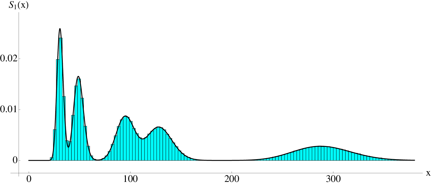
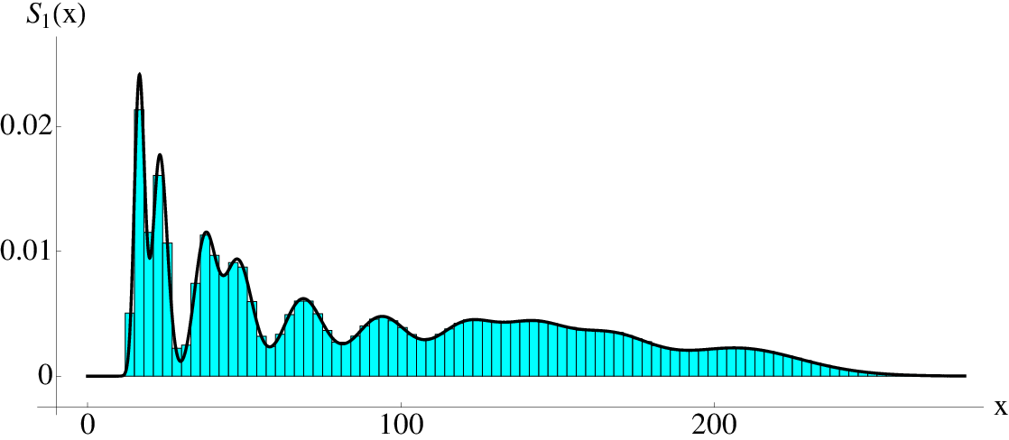
results for $p=5$ and $p=10$ and $n=200$ with the chosen empirical eigenvalues $\Lambda_{j}$, $j=1,\ldots,5$ of $\{1.44,0.64,0.49,0.25,0.16\}$ and $\Lambda_{j}$, $j=1,\ldots,10$ of $\{1,0.81,0.7225,0.64,0.45,0.36,0.25,0.2025,0.1225,0.03\}$, respectively. The agreement is perfect.

In conclusion, we introduced the supersymmetry method for the first time to Wishart correlation matrices. We thereby derived exact expressions for the eigenvalue density in terms of low–dimensional integrals. This is a drastic reduction, as the original order of integrals is $np$. Our approach solves a serious mathematical obstacle in the real case. A presentation for a mathematics audience will be given elsewhere [22]. Here, we derived and discussed the formulae needed for applications. In the real case ($\beta=1$), we obtained the previously unknown exact solution in terms of a finite sum of twofold integrals. We evaluated our formula numerically and confirmed it by comparing to Monte Carlo simulations.

We thank R. Sprik for fruitful discussions as well as A. Hucht, H. Kohler, and R. Schäfer for helpful comments. One of us (TG) greatly benefitted from the Program on High Dimensional Inference and Random Matrices in 2006 at SAMSI, Research Triangle Park, North Carolina (USA). We acknowledge support from Deutsche Forschungsgemeinschaft (Sonderforschungsbereich Transregio 12).

References

- [1] C. Chatfield, The Analysis of Time Series (Chapman and Hall/CRC, Boca Raton, 2004), 6th ed.
- [2] M. Müller, G. Baier, A. Galka, U. Stephani, and H. Muhle, Phys. Rev. E 71, 046116 (2005).
- [3] P. Šeba, Phys. Rev. Lett. 91, 198104 (2003).
- [4] R. Sprik, A. Tourin, J. de Rosny, and M. Fink, Phys. Rev. B 78, 012202 (2008).
- [5] L. Laurent, P. Cizeau, J. Bouchaud, and M. Potters, Phys. Rev. Lett. 83, 1467 (1999).
- [6] R. Muirhead, Aspects of Multivariate Statistical Theory (Wiley, New York, 1982), 1st ed.
- [7] T. Guhr, A. Müller-Groeling, and H. Weidenmüller, Phys. Rep. 299, 189 (1998).
- [8] J. Silverstein, Multivariate Anal. 55, 331 (1995).
- [9] Vinayak and A. Pandey, Phys. Rev. E 81, 036202 (2010).
- [10] G. Alfano, A. Tulino, A. Lozano, and S. Verdu, Proc. IEEE Int. Symp. on Spread Spectrum Tech. and Applications (ISSSTA ’04) (2004).
- [11] S. Simon and A. Moustakas, Phys. Rev. E 69, 065101 (2004).
- [12] K. Efetov, Adv. Phys. 32, 53 (1983).
- [13] J. Verbaarschot, H. Weidenmüller, and M. Zirnbauer, Phys. Rep. 129, 367 (1985).
- [14] K. Efetov, Supersymmetry in Disorder and Chaos (Cambridge University Press, Cambridge, 1997), 1st ed.
- [15] Harish-Chandra, Am. J. Math. 80, 241 (1958).
- [16] C. Itzykson and J. Zuber, J. Math. Phys. 21, 411 (1980).
- [17] I. Gelfand, Dokl. Akad. Nauk. SSSR 70, 5 (1950).
- [18] I. Macdonald, Symmetric Functions and Hall Polynomials (Clarendon Press, Oxford, 1998), 2nd ed.
- [19] M. Kieburg, J. Grönqvist, and T. Guhr, J.Phys. A 42, 275205 (2009).
- [20] F. Berezin, Introduction to Superanalysis (D. Reidel Publishing Company, Dordrecht, 1987), 1st ed.
- [21] Wolfram Research Inc., Mathematica Version 7.0, Champaign, Illinois (2008).
- [22] C. Recher, M. Kieburg, and T. Guhr, in preparation (2010).