Numerical methods for an optimal order execution problem Thanks: We would like to thank J.G. Grebet (EXQIM) for discussions and remarks during the preparation of this work.
Abstract
This paper deals with numerical solutions to an impulse control problem arising from optimal portfolio liquidation with bid-ask spread and market price impact penalizing speedy execution trades. The corresponding dynamic programming (DP) equation is a quasi-variational inequality (QVI) with solvency constraint satisfied by the value function in the sense of constrained viscosity solutions. By taking advantage of the lag variable tracking the time interval between trades, we can provide an explicit backward numerical scheme for the time discretization of the DPQVI. The convergence of this discrete-time scheme is shown by viscosity solutions arguments. An optimal quantization method is used for computing the (conditional) expectations arising in this scheme. Numerical results are presented by examining the behaviour of optimal liquidation strategies, and comparative performance analysis with respect to some benchmark execution strategies. We also illustrate our optimal liquidation algorithm on real data, and observe various interesting patterns of order execution strategies. Finally, we provide some numerical tests of sensitivity with respect to the bid/ask spread and market impact parameters.
Keywords: Optimal liquidation, Impulse control problem, Quasi-variational inequality, explicit backward scheme, quantization method, viscosity solutions.
JEL Classification : G11.
MSC Classification (2000) : 93E20, 65C05, 91B28, 60H30.
1 Introduction
Portfolios managers define “implementation shortfall” as the difference in performance between a theoretical trading strategy and the implemented portfolio. In a theoretical strategy, the investor observes price displayed by the market and assumes that trades will actually be executed at this price. Implementation shortfall measures the distance between the realized transaction price and the pre-trade decision price. Indeed, the investor has to face several adverse effects when executing a trading strategy, usually referred to as trading costs. Let us describe the three main components of these illiquidity effects: the bid/ask spread, the broker’s fees and the market impact. The best bid (resp. best ask) price is the best offer to buy (resp. to sell) the asset, and the bid/ask spread is the difference (always positive in the continuous trading session) between the best ask price and best bid price. The broker’s fees are the amount paid to the broker for executing the order. The market impact refers to the following phenomenon: any buy or sell market order passed by an investor induces an adverse market reaction that will penalize quoted price from the investor point of view.
Market impact is a key factor when executing large orders. A famous worst case example is Jérome Kerviel’s liquidation portfolio, operated by Société Générale in 2008. According to the report of Commission Bancaire, the liquidative value of Kerviel’s portfolio was -2,7G€ when the Société Générale decided to unwind it on January 20, 2008. The liquidation was operated during 3 days and led to a supplementary loss of 3,6G€. Even in regular operations, price impact may noticeably affect a trading strategy. On April 29, 2010, Reuters agency reports that Citadel Investment Group sold 170M shares of the E*Trade stock, and raised about 301M$: this operation led to a price fall of 7,1%. These examples explain why measurement and efficient management of market impact is a key issue for financial institutions, and the research of low-touch trading strategies has found a great interest among academics.
Most of market places and brokers offer several common tools to reduce market impact. We can cite as an example the simple time slicing (we will refer to this example later as the uniform strategy): a large order is split up in multiple children orders of the same size, and these children orders are sent to the market at regular time intervals. Brokers also propose more sophisticated tools as smart order routing (SOR) or volume weighted average price (VWAP) based algorithmic strategies. Indeed, one basic observation is that market impact can be reduced by splitting up a large order into several children orders. Then the investor has to face the following trade-off: if he chooses to trade immediately, he will penalize his performance due to market impact; if he trades gradually, he is exposed to price variation on the period of the operation. Our goal in this article is to provide a numerical method to find optimal schedule and associated quantities for the children orders.
Recently, there has been considerable interest for this problem in the academic literature. The seminal papers [5] and [2] first provided a framework for managing market impact in a discrete-time model. The optimality is determined according to a mean-variance criterion, and this leads to a static strategy, in the sense that it is independent of the stock price. Models of market impact based on stylized order book dynamics were proposed in [15], [19] and [9]. There also has been several optimal control approaches to the order execution problem, using a penalizing function to model price impact: the papers [18] and [8] assume continuous-time trading, and use an Hamilton-Jacobi-Bellman approach for the mean-variance criterion, while [10], [13], and [11] consider real trading taking place in discrete-time by using an impulse control approach. This last approach combines the advantages of realistic modelling of portfolio liquidation and the tractability of continuous-time stochastic calculus. In these papers, the optimal liquidation strategies are price-dependent in contrast with static strategies.
In this article, we adopt the model investigated in [11]. Let us describe the main features of this model. The stock price process is assumed to follow a geometrical Brownian motion. The price impact is modelled via a nonlinear transaction costs function, that depends both on the quantity traded, and on a lag variable tracking the time spent since the investor’s last trade. This lag variable will penalize rapid execution trades, and ensures in particular that trading times are strictly increasing, which is consistent with market practice in limit order books. In this context, we consider the problem of an investor seeking to unwind an initial position in stock shares over a finite horizon. Risk aversion of the investor is modelled through a utility function, and we use an impulse control approach for the optimal order execution problem, which consists in maximizing the expected utility from terminal liquidation wealth, under a natural economic solvency constraint involving the liquidation value of portfolio. The theoretical part of this impulse control problem is studied in [11], and the solution is characterized through dynamic programming by means of a quasi-variational inequality (QVI) satisfied by the value function in the (constrained) viscosity sense. The aim of this paper is to solve numerically this optimal order execution problem. There are actually few papers dealing with a complete numerical treatment of impulse control problems, see [6], [14], or [7]. In these papers, the domain has a simple shape, typically rectangular, and a finite-difference method is used. In contrast, our domain is rather complex due to the solvency constraint naturally imposed by the liquidation value under market impact, and we propose a suitable probabilistic numerical method for solving the associated impulse control problem. Our main contributions are the following:
- •
We provide a numerical scheme for the QVI associated to the impulse control problem and prove that this method is monotone, consistent and stable, hence converges to the viscosity solution of the QVI. For this purpose, we adapt a proof from [4].
- •
We take advantage of the lag variable to provide an explicit backward scheme and then simplify the computation of the solution. This contrasts with the classical approach by iterative sequence of optimal stopping problems, see e.g. [6].
- •
We provide the detailed computational probabilistic algorithm with an optimal quantization method for the approximation of conditional expectations arising in the backward scheme.
- •
We provide several numerical tests and statistics, both on simulated and real data, and compare the optimal strategy to a benchmark of two other strategies: the uniform strategy and the naive one consisting in the liquidation of all shares in one block at the terminal date. We also provide some sensitivity numerical analysis with respect to the bid/ask spread and market impact parameters.
This paper is organized as follows: Section 2 recalls the problem formulation and main properties of the model, in particular the PDE characterization of the impulse control problem by means of constrained viscosity solutions to the QVI, as stated in [11]. Section 3 is devoted to the time discretization and the proof of convergence of the numerical scheme. Section 4 provides the numerical algorithm and numerical methods to solve the DPQVI. Section 5 presents the results obtained with our implementation, both on simulated and historical data.
2 Problem formulation
2.1 The model of portfolio liquidation
We consider a financial market where an investor has to liquidate an initial position of shares of risky asset by time . He faces the following risk/cost tradeoff: if he trades rapidly, this results in higher costs due to market impact; if he splits the order into several smaller blocks, he is exposed to the risk of price depreciation during the trading horizon. We adopt the recent continuous-time framework of [11], who proposed a modeling where trading takes place at discrete random times through an impulse control formulation, and with a temporary price impact depending on the time interval between trades, and including a bid-ask spread.
Let us recall the details of the model. We set a probability space equipped with a filtration supporting a one-dimensional Brownian motion on a finite horizon , . We denote by the market price of the risky asset, by the cash holdings, by the number of stock shares held by the investor at time and by the time interval between and the last trade before .
Trading strategies. We assume that the investor can only trade at discrete time on . This is modelled through an impulse control strategy where are stopping times representing the trading times and , , are -measurable random variables valued in and giving the quantity of stocks purchased if or selled if at these times. A priori, the sequence may be finite or infinite. We introduce the lag variable tracking the time interval between trades, which evolves according to
| (2.1) |
The dynamics of the number of stock shares is then given by :
| (2.2) |
Cost of illiquidity. The market price of the risky asset process follows a geometric Brownian motion:
| (2.3) |
with constant and . We do not consider a permanent price impact, i.e. the lasting effect of large trade, but focus here on the temporary price impact that penalize the price at which an investor will trade the asset. Suppose now that the investor decides at time to trade the quantity . If the current market price is , and the time lag from the last order is , then the price he actually get for the order is:
| (2.4) |
where is a temporary price impact function from into . Actually, in the rest of the paper, we consider a function in the form
| (2.5) |
where is the price impact exponent, is the temporary price impact factor, , and are the bid and ask spread parameters. The impact of liquidity modelled in (2.4) is like a transaction cost combining nonlinearity and proportionality effects. The nonlinear costs come from the dependence of the function on , but also on . On the other hand, this transaction cost function can be determined implicitly from the impact of a market order placed by a large trader in a limit order book, as explained in [15], [19] or [18]. Moreover, the dependance of in in (2.5) means that rapid trading has a larger temporary price impact than slower trading. Such kind of assumption is also made in the seminal paper [2], and reflects stylized facts on limit order books. The form (2.5) was suggested in several empirical studies, see [12], [17], [3], and used also in [8], [11].
Cash holdings. We assume a zero risk-free return, so that the cash holdings are constant between two trading times:
| (2.6) |
When a discrete trading occurs at time , this results in a variation of the cash amount given by due to the illiquidity effects. In other words, we have
| (2.7) |
Remark 2.1
Notice that since if and if , an immediate sale does not increase the cash holdings, i.e. , while an immediate purchase leads to a bankruptcy i.e. .
Liquidation value and solvency constraint. The solvency constraint is a key issue in portfolio choice problem. The point is to define in an economically meaningful way what is the portfolio value of a position in cash and stocks. In our context, we first impose a no-short selling constraint on the trading strategies, i.e.
Next, we introduce the liquidation function representing the value that an investor would obtain by liquidating immediately his stock position by a single block trade, when the pre-trade price is and the time lag from the last order is . It is defined on by
and we constrain the portfolio’s liquidative value to satisfy the solvency criterion:
We then naturally introduce the solvency region:
and we denote its boundary and its closure by
| and |
where
In the sequel, we also introduce the corner lines in :
Admissible trading strategies. Given , we say that the impulse control strategy is admissible, denoted by , if , , , and the process solution to (2.1)-(2.2)-(2.3)-(2.6)-(2.7), with an initial state (and the convention that if ), satisfies for all . As usual, to alleviate notations, we omit the dependence of in , when there is no ambiguity.
Portfolio liquidation problem. We consider a utility function from into , strictly increasing, concave and w.l.o.g. , and s.t. there exists , :
The problem of optimal portfolio liquidation is formulated as
| (2.8) |
where . As observed in [11], one can shift the terminal liquidation constraint in to a terminal liquidation utility by considering the function defined on by:
Then, problem (2.8) is written equivalently in
| (2.9) |
2.2 PDE characterization
The dynamic programming Hamilton-Jacobi-Bellman (HJB) equation corresponding to the stochastic control problem (2.8) is a quasi-variational inequality written as
| (2.10) |
together with the relaxed terminal condition
| (2.11) |
Here, is the infinitesimal generator associated to the process in a no-trading period:
is the impulse operator defined by
is the impulse transaction function defined from into :
and the set of admissible transactions :
By standard arguments, we derive the constrained viscosity solution property of the value function to (2.10)-(2.11). However, in order to have a complete characterization of the value function via its HJB equation, we need a uniqueness result. Unfortunately, in our model, it seems not possible to get such result, at least by classical arguments since there is no strict supersolution to (2.10). In [11], the authors prove a weaker characterization of the value function in terms of minimal solution to its HJB equation. They also consider a small variation of the original model by adding a fixed transaction fee at each trading. This means that given a trading strategy , the controlled state process jumps now at time , by:
| (2.12) |
where is the function defined on into by:
for . The dynamics of between trading dates is given as before. We introduce a modified liquidation function defined by:
The interpretation of this modified liquidation function is the following. Due to the presence of the transaction fee at each trading, it may be advantageous for the investor not to liquidate his position in stock shares (which would give him ), and rather bin his stock shares, by keeping only his cash amount (which would give him ). Hence, the investor chooses the best of these two possibilities, which induces a liquidation value .
The corresponding solvency region with its closure , and boundary are given by:
The set of admissible trading strategies is defined as follows: given , we say that the impulse control is admissible, denoted by , if , , , and the controlled state process solution to (2.1)-(2.2)-(2.3)-(2.6)-(2.12), with an initial state (and the convention that if ), satisfies for all . Here, we stress the dependence of in appearing in the transaction function , and we notice that it affects only the cash component.
The liquidation utility function in this model with fixed transaction fee is defined on by , and the associated optimal portfolio liquidation problem is defined via its value function by:
| (2.13) |
The dynamic programming equation associated to the control problem (2.13) is
| (2.14) | |||||
| (2.15) |
where is the impulse operator defined by
for any locally bounded function on , with the convention that when , and the set of admissible transactions in the model with fixed transaction fee is:
We recall from [11] that is in the set of functions satisfying the growth condition:
Remark 2.2
The function is strictly increasing in the argument of cash holdings , for , and fixed . Indeed, for , and , , any strategy with corresponding state process , is also in , and leads to an associated state process . Using the fact that the utility function is strictly increasing, we deduce that . Moreover, the function is nondecreasing in the argument of number of shares . Indeed, fix , and with . Given any arbitrary , consider the strategy , starting from at time , which consists in trading again immediately at time by selling shares (which does not change the cash holdings, see Remark 2.1), and then follow the same strategy than . The corresponding state process satisfies a.s. for , and in particular , together with . Since is arbitrary in , this shows that .
In the sequel, we shall denote by the set of functions in such that is strictly increasing in and nondecreasing in .
Remark 2.3
Fix . For , and s.t. , the set of admissible transactions (and for ) if , and is empty otherwise. Thus, if , and is equal to otherwise. This implies in particular that
| (2.16) |
for any , which is the case of (see Remark 2.2). Therefore, due to the market impact function in (2.5) penalizing rapid trades, it is not optimal to trade again immediately right after some trade, i.e. the optimal trading times are strictly increasing.
A main result in [11] is to provide a unique PDE characterization of the value functions , , and to prove that the sequence converges to the original value function as goes to zero.
Theorem 2.1
(1) The sequence is nonincreasing, and converges pointwise on towards as goes to zero, with .
3 Time discretization and convergence analysis
In this section, we fix , and we study time discretization of the QVI (2.14)-(2.15) characterizing the value function . For a time discretization step on the interval , let us consider the following approximation scheme:
| (3.1) |
where is defined by
| (3.2) | |||||
Here, denotes the state process starting from at time , and without any impulse control strategy: it is given by
with the solution to (2.3) starting from at time . Notice that (3.1) is formulated as a backward scheme for the solution through:
| (3.4) | |||||
| (3.5) |
and for . This approximation scheme seems a priori implicit due to the nonlocal obstacle term . This is typically the case in impulse control problems, and the usual way (see e.g. [6], [14]) to circumvent this problem is to iterate the scheme by considering a sequence of optimal stopping problems:
starting from . Here, we shall make the numerical scheme (3.1) explicit, i.e. without iteration, by taking effect of the state variable in our model. Recall indeed from Remark 2.3 that it is not optimal to trade again immediately right after some trade. Thus, for , and any , we have from (2.16) and (3.4)-(3.5):
Therefore, by using again the definition of in the relations (3.4)-(3.5), we see that the scheme (3.1) is written equivalently as an explicit backward scheme:
| (3.6) | |||||
| (3.7) |
for , and for , where we denote in (3.7) to alleviate notations. Notice that at this stage, this approximation scheme is not yet fully implementable since it requires an approximation method for the expectations arising in (3.7). This is the concern of the next section.
We focus now on the convergence (when goes to zero) of the solution to (3.1) towards the value function solution to (2.14)-(2.15). Following [4], we have to show that the scheme in (3.2) satisfies monotonicity, stability and consistency properties. As usual, the monotonicity property follows directly from the definition (3.2) of the scheme.
Proposition 3.1
(Monotonicity)
For all , , , and , s.t. , we have
We next prove the stability property.
Proposition 3.2
(Stability)
For all , there exists a unique solution to (3.1), and the sequence is uniformly bounded in : there exists s.t. for all .
Proof. The uniqueness of a solution to (3.1) follows from the explicit backward scheme (3.6)-(3.7). For , denote by the integer part of , and the partition of the interval with time step . For , we denote by the subset of elements in such that the trading times are valued in . Let us then consider the impulse control problem
| (3.8) |
It is clear from the representation (3.8) that for all , , which shows that the sequence is uniformly bounded in . Moreover, similarly as for , and by the same arguments as in Remark 2.2, we see that is strictly increasing in and nondecreasing in for . Finally, we observe that the numerical scheme (3.1) is the dynamic programming equation satisfied by the value function . This proves the required stability result.
We now move on the consistency property.
Proposition 3.3
(Consistency)
(i) For all and , we have
| (3.9) | |||||
and
| (3.10) | |||||
(ii) For all and , we have
| (3.11) | |||||
and
| (3.12) | |||||
Proof. The arguments are standard, and can be adapted e.g. from [6] or [7]. We sketch the proof, and only show the inequality (3.9) since the other ones are derived similarly. Fix . Since the minimum of two upper-semicontinous (usc) functions is also usc and using the caracterization of usc functions, we have
| (3.13) | |||||
where the last inequality follows from the continuity of and the lower semicontinuity of . Moreover, by Itô’s formula applied to , and standard arguments of localization to remove in expectation the stochastic integral, we get
Substituting into (3.13), we obtain the desired inequality (3.9).
Since the numerical scheme (3.1) is monotone, stable and consistent, we can follow the viscosity solutions arguments as in [4] to prove the convergence of to , by relying on the PDE characterization of in Theorem 2.1 (2), and the strong comparison principle for (2.14)-(2.15) proven in [11].
Theorem 3.1
(Convergence) The solution of the numerical scheme (3.1) converges locally uniformly to on .
Proof. Let and be defined on by
We first see that and are respectively viscosity subsolution and supersolution of (2.14)-(2.15). These viscosity properties follow indeed, by standard arguments as in [4] (see also [6] or [7] for impulse control problems), from the monotonicity, stability and consistency properties. Details can be obtained upon request to the authors. Moreover, from (3.8), we have the inequality: , which implies by (2.17):
| (3.14) |
Thus, by using the strong comparison principle for (2.14)-(2.15) stated in Theorem 5.2 [11], we deduce that on and so on . This proves the required convergence result.
4 Numerical Algorithm
Let us consider a time step , , and denote by the regular grid over the interval . We recall from the previous section that the time discretization of step for the QVI (2.14)-(2.15) leads to the convergent explicit backward scheme:
for , . Recall that the variable represents the time lag between the current time and the last trade. Thus, it suffices to consider at each time step of , a discretization for valued in the time grid
On the other hand, the above scheme involves nonlocal terms in the variable for the solution in relation with the supremum over and the expectations in (4)-(4), and thus the practical implementation requires a discretization for the state variable , together with an interpolation. For any , let us denote by
For the discretization of the state variable , and since is unbounded, we first localize the domain by setting , where in , , are fixed constants, and then define the regular grid:
where is the uniform grid on of step , and similarly for , .
Optimal quantization method. Let us now describe the numerical procedure for computing the expectations arising in (4). Recalling that , this involves only the expectation with respect to the price process, assumed here to follow a Black-Scholes model (2.3). We shall then use an optimal quantization for the standard normal random variable , which consists in approximating the distribution of by the discrete law of a random variable of support , and defined as the projection of on the grid according to the closest neighbour. The grid is optimized in order to minimize the distorsion error, i.e. the quadratic norm between and . This optimal grid and the associated weights are downloaded from the website: http://87.106.220.249/n01. We refer to the survey article [16] for more details on the theoretical and computational aspects of optimal quantization methods. From (4), we have to compute at any time step , and for any , , expectations in the form:
that we approximate by
| (4.9) |
Interpolation procedure. Notice that for implementing recursively in (4) this quantization method, we need to compute on given the known values of on . This approximation is achieved as follows:
- •
if , then we use a linear interpolation of with respect to the closest neighbours in .
- •
if , we use the growth condition satisfied by the value function:
where is the projection of (according to the closest neighbour) on the grid .
Algorithm description. In summary, our numerical scheme provides an algorithm for computing approximations of the value function, and of the optimal trading strategy at each time step , and each point of the grid . The parameters in the algorithm are:
- the maturity
- and the Black and Scholes parameters of the stock price
- the impact parameter, the impact exponent in the market impact function (2.5)
- , the spread parameters in percent, the transactions costs fee
- We take by default a CRRA utility function:
- , , , the boundaries of the localized domain
- number of steps in time discretization, the number of steps in space discretization
- number of points for optimal quantization of the normal law, number of points used in the static supremum in
The algorithm is described explicitly in backward induction as follows:
Initialization step at time :
- •
(s:0) For , set , on , and interpolate on .
- •
(s:j) For ,
- –
for , compute and denote by the argument maximum:
- –
if , then set and ,
- –
else set , and .
- –
Interpolate on .
- –
5 Numerical Results
5.1 Procedure
For each of the numerical tests, we used the same procedure consisting in the following steps:
(1) Set the parameters according to the parameter table described in the first subsection of each test
(2) Compute and save the grids representing value function and optimal policy according to the optimal liquidation algorithm
(3) Generate paths for the stock price process following a geometrical Brownian motion: we choose parameters and that allows us to observe several empirical facts on the performance and the behavior of optimal liquidation strategy. These parameters can also be estimated from historical observations on real data by standard statistical methods.
(4) Consider the portfolio made of dollars and shares of risky asset
(5) For each price path realization, update the portfolio along time and price path accordingly to the policy computed in the second step
(6) Save each optimal liquidation realization
(7) Compute statistics
In the sequel, we shall use the following quantities as descriptive statistics:
- •
The performance of the -th realization of the optimal strategy is defined by
where is the state process, starting at date at , evolving under the -th price realization and the optimal control . This quantity can be interpreted as the ratio between the cash obtained from the optimal liquidation strategy and the ideal Merton liquidation. We define in the same way the quantities and respectively associated with the controls and of the naive and uniform strategy, refereed as benchmark strategies. Recall that the naive strategy consists in liquidating the whole portfolio in one block at the last date, and the uniform strategy consists in liquidating the same quantity of asset at each predefined date until the last date. Notice that the score corresponds to the strategy, which consists in liquidating the whole portfolio immediately in an ideal Merton market.
When denoting by the number of paths of our simulation, we define:
- •
The mean utility
- •
The mean performance
- •
The standard deviation of the strategy
Here the dot . stands for , or . We will also compute the third and fourth standardized moments for the series .
5.2 Test 1: A toy example
The goal of this test is to show the main characteristics of our results. We choose a set of parameters that is unrealistic but that has the advantage of emphasizing the typical behavior of the optimal liquidation strategy.
Parameters
We choose the set of parameters shown in table 1.
| Parameter | Value | Parameter | Value |
|---|---|---|---|
| Maturity | 1 year | 2000 | |
| 5.00E-07 | 2500 | ||
| 0.5 | 5.0 | ||
| 0.5 | -30000 | ||
| 1.01 | 80000 | ||
| 0.99 | 0 | ||
| 0.001 | 5000 | ||
| 0.1 | 0 | ||
| 0.5 | 20 | ||
| 40 | |||
| 20 | |||
| 100 | |||
Execution statistics
The results were computed using Intel® Core 2 Duo at 2.93Ghz CPU with 2.98 Go of RAM. Statistics are shown in table 2.
| Quantity | Evaluation |
|---|---|
| Time Elapsed for grid computation in seconds | 7520 |
| Number Of Available Processors | 2 |
| Estimated Memory Used (Upper bound) | 953MB |
| Time Elapsed for statistics Computation in seconds | 21 |
Shape of policy
In this paragraph we plotted the shape of the policy sliced in the plane , i.e. the (cash, shares) plane, for a fixed (figure 1). The color of the map at on the graph represents the action one has to take when reaching the state . We can see three zones: a buy zone (denoted BUY on the graph), a sell zone (denoted SELL on the graph) and a no trade zone (denoted NT on the graph). Note that the bottom left zone on the graph is outside the domain . These results have the intuitive financial interpretation: when is big and is small, the investor has enough cash to buy shares of the risky asset and tries to profit from an increased exposure. When is large and is small, the investor has to reduce exposure to match the terminal liquidation constraint.
We also plotted the shape of the policy sliced in the plane , i.e. the (shares,price) plane, for a fixed (figure 2). As before, the color of the map at on the graph represents the action one has to take when reaching the state . Again, we can distinguish the three zones: buy, sell and no trade.
Shape of value function
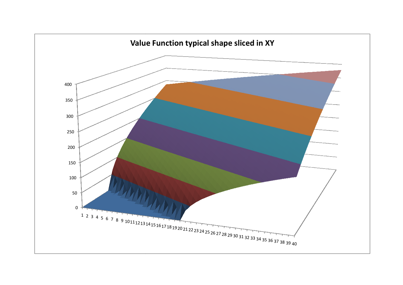
Figure 3 shows the value function sliced in the plane. This figure is a typical pattern of the value function. Recall from Proposition 3.1 in [11]) the following Merton theoretical bound for the value function:
In the figure 4 we plotted the difference between the value function and this theoretical bound. We observe that this difference is increasing with the number of shares, and decreasing with the cash. This result is interpreted as follows: the price impact increases with the number of shares, but this can be reduced by the liquidation strategy whose efficiency is greater if the investor can sustain bigger cash variations.
5.3 Test 2: Short term liquidation
The goal of this test is to show the behavior of the algorithm on a realistic set of parameters and real data. We used Reuters data fed by OneTick TimeSeries Database. We used the spot prices (Best Bid and Best Ask) for the week starting 04/19/2010 on BNP.PA. We computed mid-price that is the middle between best bid and best ask price. We choose the impact parameter in order to penalize by approximately 1% the immediate liquidation of the whole portfolio compared to Merton liquidation. In other words, we take so that: .
Parameters
We computed the strategy with parameters shown in table 3.
| Parameter | Value | Parameter | Value |
|---|---|---|---|
| Maturity | 1 Day | 20000 | |
| 5.00E-04 | 2500 | ||
| 0.2 | 52.0 | ||
| 0.5 | -30000 | ||
| 1.0001 | 200000 | ||
| 0.9999 | 0 | ||
| 0.001 | 5000 | ||
| 0.005 | 50.0 | ||
| 0.25 | 54.0 | ||
| 30 | |||
| 40 | |||
| 100 | |||
Execution statistics
We obtained the results using Intel® Core 2 Duo at 2.93Ghz CPU with 2.98 Go of RAM, the computations statistics are gathered in table 4.
| Quantity | Evaluation |
|---|---|
| Time Elapsed for grid computation in seconds | 8123 |
| Number Of Available Processors | 2 |
| Estimated Memory Used (Upper bound) | 573MB |
Performance Analysis
We computed the mean utility and the first four moments of the optimal strategy and the two benchmark strategies in table 5 and plotted the empirical distribution of performance in figure 5. It is remarkable that the optimal strategy gives an empirical performance that is above the immediate liquidation at date 0 in the Merton ideal market. This is due to the fact that the optimal strategy has an opportunistic behavior, as the decisions are based on the price level, and so profit from the ‘detection” of some favorable price conditions. Indeed, an optimal trading strategy is embedded with the optimal liquidation: in this example, this feature not only compensates the trading costs, but also provides an extra performance compared to an ideal immediate liquidation at date 0. Still, the Merton case is a theoretical upper bound in the following sense: the optimal value function with trading costs is below the optimal value function without trading costs, recall the figure 4. As expected, the empirical distribution is between the distributions of the two other benchmark strategies. We also notice that the optimal strategy outperforms the two others by approximatively 0.25% in utility and in performance.
| Strategy | Utility | Mean | Standard Dev. | Skewness | Kurtosis |
|---|---|---|---|---|---|
| Naive | 0.99993 | 0.99986 | 0.00429 | 0.94584 | 4.68592 |
| Uniform | 0.99994 | 0.99988 | 0.00240 | 0.42788 | 3.34397 |
| Optimal | 1.00116 | 1.00233 | 0.00436 | 1.03892 | 4.89161 |
We also computed other statistics in table 6.
| Quantity | Formula | Value |
|---|---|---|
| Winning percentage | 58.8% | |
| Relative Optimal Utility | 0.00238 | |
| Relative Optimal Performance | 0.00244 | |
| Utility Sharpe Ratio | 0.28017 | |
| Performance Sharpe Ratio | 0.56140 | |
| VaR 95% Naive Strategy | 0.994 | |
| VaR 95% Uniform Strategy | 0.996 | |
| VaR 95% Optimal Strategy | 0.997 | |
| VaR 90% Naive Strategy | 0.995 | |
| VaR 90% Uniform Strategy | 0.997 | |
| VaR 90% Optimal Strategy | 0.998 |
Behavior Analysis
In this paragraph, we analyze the behaviour of the strategy as follows: first, we plotted in figure 6 the empirical distribution of the number of trades for one trading session. Secondly, we plotted trades realizations for three days of the BNPP.PA stock for the week starting on 04/19/2010.
The three following graphs represent three days of market data for which we computed the mid-price (lines) with associated trades realizations for the optimal strategy (vertical bars). A positive quantity for the vertical bar means a buying operation, while a negative quantity means a selling operation.
Figure 7 shows the trade realizations of the optimal strategy for the day 04/19/2010 on the BNPP.PA stock. The interesting feature in this first graph is that we see two buying decisions when the price goes down through the 54.5 barrier, and which corresponds roughly to a daily minimum. The following selling decision can be viewed as a failure. On the contrary, the two last selling decisions correspond quite precisely to local maxima.
Figure 8 shows the trade realizations of the optimal strategy for the day 04/22/2010 on the BNPP.PA stock. The interesting feature in this realization is that it looks like a U-shaped pattern of liquidation that appears in [1] for an mean-variance optimal strategy with a power-law order book resilience. This pattern is very robust, so we expect that it appears frequently in the optimal strategy. Moreover, we can notice that the volume of each trade in the day is roughly increasing (in absolute value) with the current price.
Figure 9 shows the trade realizations of the optimal strategy for the day 04/23/2010 on the BNPP.PA stock. This realization is another illustration of the phenomenon of “maxima detection” that appears when executing the optimal strategy. Note that in this last realization, the naive strategy was overperforming the optimal strategy, due to an unexpected price increase. Despite this, it is satisfactory to see that there are only three trades, which is less than on April 19 and 22, 2010, and that the detection of favorable price is accurate.
5.4 Test 3: Sensitivity to Bid/Ask spread
In this last section, we are interested in the sensitivity of the results to the bid/ask spread, determined here by the two parameters and . More precisely, we look at the dominant effect between the spread and the multiplicative price impact through the parameter . We proceeded to two tests here: one without bid/ask spread, i.e. and with as before, and one with a spread of and a price impact parameter .
Parameters
The table 7 shows the parameters of the two tests. We only changed the impact and spread parameters and let the others be identical.
| Parameter | No spread test | No impact test | Parameter | No spread test | No impact test |
|---|---|---|---|---|---|
| Maturity | 1 Day | 1 Day | 20000 | 20000 | |
| 5.00E-04 | 0 | 2500 | 2500 | ||
| 0.2 | 0 | 51 | 51 | ||
| 0.5 | 0.5 | -20000 | -20000 | ||
| 1 | 1.001 | 200000 | 200000 | ||
| 1 | 0.999 | 0 | 0 | ||
| 0.001 | 0.001 | 5000 | 5000 | ||
| 0.01 | 0.01 | 49 | 49 | ||
| 0.25 | 0.25 | 53 | 53 | ||
| 30 | 30 | ||||
| 40 | 40 | ||||
| 100 | 100 | ||||
Performance Analysis
In table 8 we computed several statistics on the results. In figure 10 we plotted the empirical distribution of performance in the two tests, with the test 2 distribution (Cf. figure 5) serving as a reference. In figure 11 we plotted the empirical distribution of the number of trades in the two tests, which is particularly helpful for interpreting the results. Indeed, we see that a big spread reduces the number of trades of the optimal strategy. This can be interpreted as a phenomenon of clustering, which is consistent with the financial interpretation: if the spread is very large, the opportunity to buy at low price and sell at high price is significantly reduced, and more risky. Moreover, a large spread penalizes strategies that both buy or sell frequently. Then the optimal strategy tends to execute bigger quantity in a single trade, supported by the absence of price impact. This has the side effect of enlarging the distribution of the optimal strategy in this case, since the number of trades tends to decrease. Indeed, we observe that the smallest standard deviation is obtained with the uniform strategy, and the largest one is obtained with the naive strategy, then, qualitatively speaking, we expect the standard deviation of performance to decrease with the number of trades. On the other hand, setting the spread to zero does not change the shape of the empirical distribution, and comparing table 8 with tables 5 and 6, we see that there is almost no change between zero spread and a one-tick spread. This result may be interpreted as follows: first, we notice that there is an approximation in the state space, and particularly in the price grid, due to our discretization, which is bigger than the scale of one tick (one tick is the price discretization unit in the market’s limit order book, typically 0.01€). One finer study would be to set the prices grid precisely on the market’s prices grid. However, as mentioned before, the special feature of our strategy is the path-dependency. Let us consider the typical scale of quantities involved in our optimization: we expect the optimal strategy to profit from price variation at the scale of 1€ in our example; if the spread is about 0.1€, like in our last example, and if we usually do about 10 trades on the liquidation period, the effect of the spread ( €= 1€) is at the same scale as the price fluctuation. Then, the spread will have an important penalizing impact on the optimal trading strategy, and particularly on its schedule, i.e. the trading times (the quantities traded are more specifically constrained by market impact). On the contrary, if the spread remains small compared to the price fluctuations, the optimal trading schedule is not really modified, and the aspect of the performance distribution has a similar form.
| Quantity | No spread test | No impact test | No spread vs. T2 | No impact vs. T2 |
|---|---|---|---|---|
| Mean Utility | 1.00113 | 1.00025 | ||
| Mean Performance | 1.00227 | 1.00053 | ||
| Standard Deviation | 0.00432 | 0.00906 |
References
- [1] Alfonsi A., Schied A. and A. Slynko (2009): “Order book resilience, price manipulation, and the positive portfolio problem”, preprint
- [2] Almgren R. and N. Chriss (2001): “Optimal execution of portfolio transactions”, Journal of Risk, 3, 5-39.
- [3] Almgren R., Thum C., Hauptmann E. and H. Li (2005): “Equity market impact”, Risk, July 2005, 58-62.
- [4] Barles G. and P. Souganidis (1991): “Convergence of approximation schemes for fully nonlinear second order equations”, Asymptotic Analysis, 4, 271?283.
- [5] Bertsimas D. and A. Lo (1998): “Optimal control of execution costs”, Journal of Financial Markets, 1, 1-50.
- [6] Chancelier J.P., Oksendal B. and A. Sulem (2002): “Combined stochastic control and optimal stopping, and application to numerical approximation of combined stochastic and impulse control”, Tr. Mat. Inst. Steklova, 237(Stokhast. Finans. Mat.), 149?172.
- [7] Chen Z. and and P.A. Forsyth (2008): “A numerical scheme for the impulse control formulation for pricing variable annuities with a guaranteed minimum withdrawal benefit (gmwb)”, Numerische Mathematik, 109, 535-569.
- [8] Forsyth P. (2009): “A Hamilton-Jacobi-Bellman approach to trade execution”, preprint, University of Waterloo.
- [9] Gatherai J., Schied A. and A. Slynko (2010): “Transient linear price impact and Fredholm integral equations”, preprint
- [10] He H. and H. Mamaysky (2005): “Dynamic trading policies with price impact”, Journal of Economic Dynamics and Control, 29, 891-930.
- [11] Kharroubi I. and H. Pham (2009): “Optimal portfolio liquidation with execution cost and risk”, Preprint, University Paris 7, LPMA.
- [12] Lillo F., Farmer J. and R. Mantagna (2003): “Master curve for price impact function”, Nature, 421, 129-130.
- [13] Ly Vath V., Mnif M. and H. Pham (2007): “A model of optimal portfolio selection under liquidity risk and price impact”, Finance and Stochastics, 11, 51-90.
- [14] Maroso S. (2006): Analyse numérique de problèmes de contrôle stochastique, PhD thesis, University Paris 6.
- [15] Obizhaeva A. and J. Wang (2005): “Optimal trading strategy and supply/demand dynamics”, to appear in Journal of Financial Markets.
- [16] Pagès G., Pham H and J. Printems (2004): ”Optimal quantization methods and applications to numerical problems in finance”, Handbook of computational and numerical methods in finance, ed. Z. Rachev, Birkhauser.
- [17] Potters M. and J.P. Bouchaud (2003): “More statistical properties of order books and price impact”, Physica A, 324, 133-140.
- [18] Rogers L.C.G. and S. Singh (2008): “The cost of illiquidity and its effects on hedging”, to appear in Mathematical Finance.
- [19] Schied A. and T. Schöneborn (2009): “Risk aversion and the dynamics of optimal liquidation strategies in illiquid markets”, Finance and Stochastics, 13, 181-204.