Topological Transition of Graphene from Quantum Hall Metal to Quantum Hall Insulator at $\nu=0$

Introduction. —The intriguing quantum Hall effect (QHE) in graphene has attracted a lot of attentions in recent years [1, 2]. The quantum Hall (QH) plateaus was initially found to be [3] $\sigma_{xy}=(4e^{2}/h)(n+1/2)=\nu e^{2}/h,\ n=0,\pm 1,\pm 2,...$. The result can be understood in the same manner as the QHE in usual two-dimensional electron gases with graphene’s special properties [3, 4]: The factor of 4 comes from spin and valley (so-called $K$ and $K^{\prime}$ points) degeneracy, and 1/2, in the terminology of edge states, is from the interesting splitting of $n=0$ Landau level (LL) at sample edges due to the particle-hole symmetry [4]. This QHE rule was soon violated in stronger fields, and anomalous plateaus of $\nu=0,\pm 1$ [5] due to the breaking of spin and valley degeneracy were discovered although the detailed symmetry-breaking mechanisms are still under debate [6]. The recent surprise comes from the discovery of insulating phase at charge neutral point (CNP) in a high magnetic field $B$ by Checkelsky et. al [7] because it disagrees with the early appealing theory [4] that explained well all existing experiments then. This discovery was confirmed by the temperature-dependence study of magneto-transport near CNP (zero-energy) by Zhang et. al [8]. Experiments [7, 8] reveal following universal features. 1) Depending on the sample quality and applied field, graphene at CNP in QH regime can be either a QH-metal or a QH-insulator (see below). 2) A magnetic field can drive a graphene at CNP from the QH-metal state at relative low field into the QH-insulator state at high enough field. The critical field required for such a transition is lower for a higher quality sample. 3) The nature of the transition seem to be Kosterlitz-Thouless type (KT-type).

Two possible $n=0$ states have been proposed and examined. One is the QH-metal [4] that occurs when spin split is larger than the valley split as illustrated in Fig. 1(a). The $n=0$ LL splits first into spin-up (blue curves) LL and spin-down (red curves) LL. The further splits of valley degeneracy near the sample edges create two counter-propagating charge and spin carrying edge channels, which results in a residual conductance of $2e^{2}/h$. This is a topological state protected by the electron-hole symmetry [4]. The other possibility is the QH-insulator when the valley degeneracy lifts first with a smaller spin split primarily due to the Zeeman effect. As shown in Fig. 1(b), the $K-$LL and $K^{\prime}-$LL move symmetrically to the opposite direction of zero-energy (due to electron-hole symmetry). As a result, the topological edge channels are absent at zero energy, and a true insulator appears. The QH-insulator was previously excluded from a possible $n=0$ state mainly due to the early experimental observation of saturated longitudinal resistance at low temperature [4]. However, the recent observation of insulating phase near CNP suggests that QH-insulator is also a possible zero-energy phase of graphene [7, 8].

The mechanism of the breaking of fourfold degeneracy of $n=0$ LL has been discussed extensively in literature [6, 9, 10, 11, 12, 13, 14]. Whether graphene at zero-energy in the QH regime is described by QH-metal or QH-insulator has also been studied by Yang and Han [15]. They suggested that a graphene will be a QH-metal if spin splits first while the graphene is a QH-insulator if valley splits first. However, the study did not address why the same sample can change from a QH-metal to a QH-insulator. Assume that there is a field-induced metal-to-insulator transition, Nomura, Ryu, and Lee [16] tried to identify possible order-parameter and to argue the transition being the experimentally observed KT-type. In this letter, we would like to provide a plausible path that a graphene at CNP can change from a QH-metal state to a QH-insulator state as the magnetic field increases. The hope is not only to understand why both QH-metal and QH-insulator phases are possible in the same sample, but also to provide a guide for experimental manipulation of the transition between the two phases. We will show that bond fluctuations due to intrinsic ripples in a graphene can resist the $K$–$K^{\prime}$ split in low magnetic field, resulting in the QH-metal state at CNP. In the opposite scenario, one should expect a QH-insulator state.

Picture.— It shall be useful to first present our picture of why a transition from the QH-metal to the QH-insulator phases should be expected in graphene in a strong magnetic field. Firstly, LLs of graphene in a strong magnetic field are highly degenerated. According to Peierls instability for a solid or Jahn-Teller effect for a molecule [17], the graphene can lower its energy through a lattice distortion [18]. The degree of distortion should be proportional to the magnetic field because the LL degeneracy is proportional to the field [13, 18]. The distortion destroys $K$–$K^{\prime}$ (or sublattices A and B for $n=0$ LL) degeneracy. According to various estimation [13, 16, 18, 19], the $K$–$K^{\prime}$ split is linear in B-field for an ordered distortion, similar to the usual Zeeman effect but bigger. Although there may be other mechanism of breaking valley degeneracy such as electron-electron interaction [6, 9, 10], but the Peierls instability should be robust and universal for highly degenerated systems like graphene that can also be regarded as a large molecule. Secondly, it is inevitable to get ride of ripples in graphene. The ripples create the intrinsic bond disorders, and the intrinsic bond fluctuations tend to suppress the $K-K^{\prime}$ split in $n=0$ LL because the bond fluctuation shall restore the inversion symmetry of A- and B-sublattices [20, 21]. As a result, the lattice distortion and the intrinsic bond fluctuations compete with each other. At relative low field, the fluctuations overtake the distortion effect, and there is no $K$–$K^{\prime}$ valley splitting. The graphene at the Dirac point is a QH-metal. However, at high enough field, the Peierls-type lattice distortion dominates, and $K$–$K^{\prime}$ splitting occurs. The Dirac point becomes a QH-insulator.

Model and method. —Low energy excitations of graphene are from $\pi-$electrons that can be modeled by a tight-binding Hamiltonian on a honeycomb lattice, $H=\sum\limits_{i\sigma}\varepsilon_{i\sigma}|i\sigma><i\sigma|+\sum\limits_{<ij>,\sigma}{(t_{ij}+\delta t_{ij})e^{i\phi_{ij}}|i\sigma><j\sigma|+h.c.}$. $t_{ij}$ is the hopping energy between two nearest-neighbor sites whose value for a pure graphene is $t=-2.7eV$. $\sigma=\pm$ is spin label. $\varepsilon_{i\sigma}$ is the on-site energy that includes the Zeeman contribution $\pm g\mu_{B}B/2$ for spin-up ($+$) and spin-down ($-$), leading to a spin-gap $\Delta_{s}=g\mu_{B}B=1.3\times B[K/T]$. One can also add a random on-site energy to mimic the extrinsic disorders. $\delta t_{ij}$ is for the possible intrinsic random hopping energy described later. The magnetic field is introduced by Peierls’ substitution in hopping parameter $\phi_{ij}=2\pi e/h\int_{i}^{j}\vec{A}\cdot d\vec{l}$ [22]. The Peierls lattice distortion is either in-plane like Kekulé bond order wave[13, 16, 19], which alternates the short and long bonds like in the classical benzene molecule (see inset of Fig. 3(a)), or out-plane like charge density wave (CDW) [18], which breaks the inversion symmetry of sublattices (see inset of Fig. 3(d)). The distortion is chosen in such as way that valley gap is $\Delta_{v}=2.0\times B[K/T]$ [13, 16, 19] (for in-plane like Kekulé bond order wave) or $\Delta_{v}=4.2\times B[K/T]$ [18] (for out-plane CDW), both of which are bigger than $\Delta_{s}$.

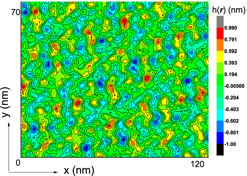
It is known that ripples (long-ranged corrugation) are the intrinsic fluctuations of graphene [23]. It is observed that the graphene ripples have a height variation of about $0.5\sim 1.0$nm, which occurs on a lateral scale of $8\sim 10$nm. The graphene with random ripples can be simulated by superposition of a series of plane waves[24]. The out-of-plane displacement is $h(\textbf{r})=C\sum\limits_{i}C_{\textbf{q}_{i}}\sin(\textbf{q}_{i}\cdot\textbf{r}+\delta_{i})$, where $\textbf{r}=(x,y)$ is the position of in-plane atoms and $C_{\textbf{q}_{i}}$, $\textbf{q}_{i}$ and $\delta_{i}$ are random numbers[25]. The lowest possible $\textbf{q}_{i}$ determines lateral scale of ripples, and the height fluctuation is controlled by $C$ value. Fig. 2 is the contour plot of one corrugated graphene used in our calculations. The random shapes and locations of ripples lead to a random change in bond length that in turn causes the hopping energy fluctuations [2]: $\delta t_{ij}=t\alpha\Delta a/a$, where $\Delta a=\sqrt{a^{2}+(h(\textbf{r})-h(\textbf{r}^{\prime}))^{2}}-a$ and $\alpha=\partial\log t/\partial\log a=2$[24].

As it was explained in our early discussions, whether a graphene is in QH-metal or QH-insulator states depends on how the valley and spin split in the bulk. Thus one needs only to study bulk states in order to determine two topologically different states. To see how $n=0$ LL split into spin bands and valley bands in the lattice distorted graphene with intrinsic random hopping, we need to obtain an accurate density of states (DOS) of the model numerically. The Lanczos recursive method [26, 27] on a large lattice (with about million lattice sites) is employed. The averaged DOS $\rho(E)=-\frac{1}{\pi}Im<\psi|\frac{1}{E-H+i\eta}|\psi>$ is computed. In the approach, a small artificial cut-off energy ($\eta=0.1meV$), which results in a small LL width in clean graphene, is introduced to simulate an infinitesimal imaginary energy [27]. A periodic boundary condition is used in order to minimize the boundary effects since our concern is the bulk $n=0$ LL splits.

Results and discussions. —Fig. 3(a-c) are the DOS of $n=0$ LL for in-plane distorted graphene of the Kekulé bond order wave (shown in the inset of Fig. 3(a)) in the presence of ripples shown in Fig. 2. At a relative low magnetic field $B=9.4T$ (Fig. 3(a)), the distortion-induced valley gap cannot compete with the hopping fluctuation so that bond order wave is statistically destroyed. As a result, $K$–$K^{\prime}$ degeneracy is statistically restored, and $n=0$ LL splits into spin-up (blue) and spin-down (red) bands due to the Zeeman energy as shown in Fig. 3(a). This is the QH-metal state discussed early because the spin splitting dominates the bulk gap of $n=0$ LL. As the magnetic field is above the critical field $B_{c}$ (between $9.4$T and $13.2$T in our case as indicated in Fig. 3(a-b)), the distortion-induced valley gap appears and $n=0$ LL splits into four bands. As shown in Fig. 3(b), two peaks on the left (right) sides of zero energy are for $K$ ($K^{\prime}$) valleys and the corresponding edge states do no cross each other. The graphene is in the QH-insulator state at CNP. Further increase of the field, the valley splits become even bigger as shown in Fig. 3(c) for $21.9$T. To shown that above result is very robust against different type of distortion, we made the same type of calculations for the CDW lattice distortion (shown in the inset of Fig. 3(d)) [18]. The similar results as those for the Kekulé bond wave have been found. As shown in Fig. 3(d-f). The valley degeneracy is preserved at $6.6$T (d) and the zero-energy state is a QH-metal. The valley degeneracy is broken at $11.0$T (e), resulting in a QH-insulator at CNP. Further increase of field to $21.9$T (f) in this case, the two $K$ ($K^{\prime}$) bands are clearly located in the same side of the zero-energy point.

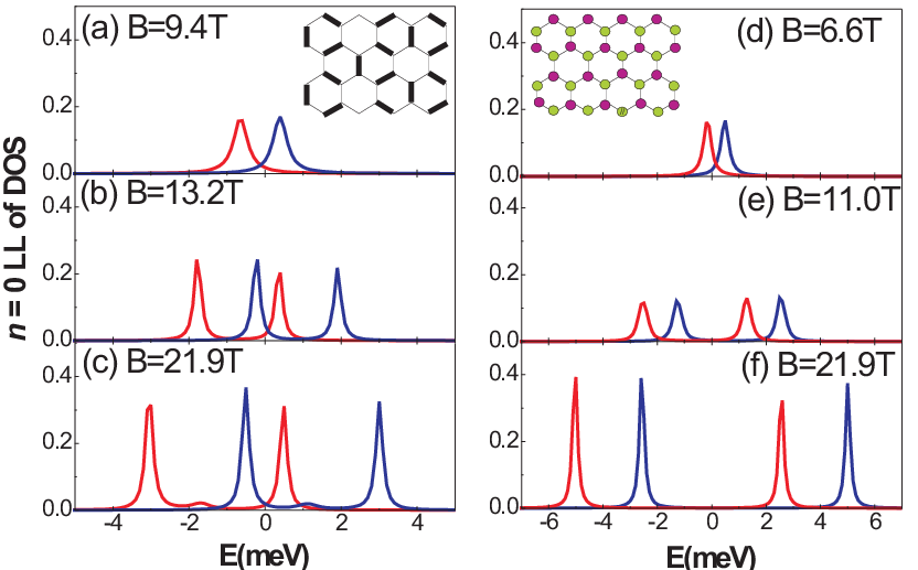
Fig. 3 shows clearly that the intrinsic bond randomness due to ripples can suppress lattice distortion-induced valley splitting no matter whether the distortion is in-plane (Kekulé bond wave) or out-plane (CDW), demonstrating the robustness and universality of the picture for grapheme. As shown from our calculations, the valley degeneracy is destroyed and valley gap appear when the bond disorder is not strong enough to restore inversion symmetry of $A$–$B$ sublattices statistically. A cleaner sample should have a weak bond disorder, and the corresponding valley degeneracy can be broken by a smaller lattice distortion. In another word, the critical field $B_{c}$ that induces the transition from the QH-metal state to the QH-insulator state depends on the degree of bond randomness. The cleaner a sample is, the smaller the critical field required to drive the graphene from the QH-metal into the QH-insulator is needed. In our model the bond randomness is measured by the height-fluctuation $h_{max}$ of ripples. Fig. 4 is $h_{max}$-dependence of the critical field $B_{c}$ for both Kekulé type and CDW-type lattice distortion. It is found that the value of $B_{c}$ of CDW type is lower than that of Kekulé type because the valley gap in CDW distortion is bigger. The inset of Fig. 4 is the phase diagram for the QH-insulator and the QH-metal. This is exactly what was observed in experiments [7, 8]. This also explains that failure of the discovery of the zero-energy insulating phase at high field in experiments before Checkelsky et. al [7] is probably due to the quality of the samples.

We would like to make a few remarks before ending this paper. 1) Fixed the applied magnetic field, the random fluctuation drives a graphene from a zero-energy insulator to a zero-energy metal. This is opposite to the role of randomness usually played in a metal-to-insulator transition. 2) There are two types of disorders in graphene, the intrinsic bond disorder due to the spontaneous ripple formation and extrinsic disorder from the impurity states in substrate [28] and/or ad-atoms [2]. The extrinsic disorder can cause the on-site-energy randomness in the tight-binding model. Our numerical studies show that the on-site disorders will not suppress the $K$–$K^{\prime}$ split, but merely broaden $K-$ and $K^{\prime}-$ subbands [12, 29]. The Landau subband broadening can cause inter-Landau-subband mixing that may change the localization property [30] of a disordered system. 3) Our QH-metal is in fact a topological insulator because it is a bulk insulator with conducting edge channels[4] while the QH-insulator is a conventional insulator. The present work is on why the magnetic field can drive such a topological transition rather than the nature of the transition [16]. 4) The Coulomb interaction is neglected here because we do not expect the change of physics by the interaction.

We present a theory of graphene for the field-driven topological transition from the QH-metal state to the QH-insulator state at $\nu=0$. The transition results from the competition between Peierls-type lattice distortion and random bond fluctuation. Our theory provides not only a clear explanation about the existence of both QH-metal state at low field and QH-insulator state at high field near the CNP, but also why the critical field for a cleaner sample is lower.

This work is supported by Hong Kong RGC grants (# 604109, HKU10/CRF/08- HKUST17/CRF/08 and SBI07/08.SC09); the NNSF of China (No. 10974187); NKBRP of China (No. 2006CB922005); and KIP of the Chinese Academy of Sciences (No. KJCX2-YW-W22).

References

- [1] K. S. Novoselov, et. al, Science 306, 666(2004).
- [2] A. K. Geim, et. al, Nat. Mater. 6, 183(2007); A. H. Castro Neto, et. al, Rev. Mod. Phys. 81, 109(2009); S. Das Sarma, et. al, arxiv-1003.4731.
- [3] K. S. Novoselov, et. al, Nature 438, 197(2005); Y. Zhang, et. al, Nature, 438, 201(2005).
- [4] D. A. Abanin, et. al, Phys. Rev. Lett. 96, 176803(2006); D. A. Abanin, et. al, ibid. 98, 196806(2007).
- [5] Y. Zhang, et. al, Phys. Rev. Lett. 96, 136806(2006); Z. Jiang, et. al, ibid. 99, 106802(2007).
- [6] K. Yang, Solid State Communications 143, 27(2007); S. Das Sarma and K. Yang, ibid. 149, 1502(2009).
- [7] J. G. Checkelsky, et. al, Phys. Rev. Lett. 100, 206801(2008);J. G. Checkelsky, et. al, Phys. Rev. B 79, 115434(2009).
- [8] Liyuan Zhang, et. al, arxiv-1003.2738.
- [9] Jason Alicea, et. al, Phys. Rev. B 74, 075422(2006).
- [10] V. P. Gusynin, et. al, Phys. Rev. B 74, 195429(2006); E. V. Gorbar, et. al, ibid. 66, 045108(2002).
- [11] Igor A. Luk’yanchuk, et. al, Phys. Rev. Lett. 100, 176404(2008).
- [12] M. Koshino and T. Ando, Phys. Rev. B 75, 033412(2007); N. H. Shon, et. al J. Phys. Soc. Jpn. 67, 2421(1998).
- [13] N. A. Viet, et. al, J. Phys. Soc. Jpn. 63, 3036(1994);H. Ajiki and T. Ando, ibid. 64, 260(1995).
- [14] Shinsei Ryu, et. al, Phys. Rev. B 80, 205319(2009).
- [15] Z. Yang, et. al, Phys. Rev. B 81, 115404(2010).
- [16] K. Nomura, et. al, Phys. Rev. Lett. 103, 216801(2009).
- [17] L. Curtiss, et. al, Phys. Rev. Lett. 69, 2435(1992).
- [18] Jean Noël Fuchs, et. al, Phys. Rev. Lett. 98, 016803(2007); J. N. Fuchs, et. al, Eur. Phys. J. Special Topics 148, 151(2007).
- [19] C. Y. Hou, et. al, Phys. Rev. B 81, 075427(2010).
- [20] Tohru Kawarabayashi, et. al, Phys. Rev. Lett. 103, 156804(2009); Tohru Kawarabayashi, et. al, Physica E, 42, 759(2010).
- [21] F. Guinea, et. al, Phys. Rev. B 77, 205421(2008).
- [22] X. R. Wang, Phys. Rev. B 51, 9310(1995); ibid. 53, 12035(1996); R. Saito, G. Dresselhaus and M. S. Dresselhaus, Physical Properties of Carbon Nanotubes, Imperial College Press, London(1998).
- [23] Elena Stolyarova, et. al, Proc. Nat. Aca. Sci. 104, 9209(2007); Jannik C. Meyer, et. al, Nature, 446, 60(2007);A. Fasolino, et. al, Nat. Mater. 6, 858(2007).
- [24] J. W. Klos, et. al, Phys. Rev. B 80, 245432(2009); S. Costamagna, et. al, Phys. Rev. B 81, 115421(2010).
- [25] The wave vectors randomly distributed in the range , where is the typical length of the system and is the lattice constant. The phase is randomly distributed in the range . for and otherwise , where , represents the averaged distance of the adjacent peaks of spatial ripples. In our calculations, there are random waves to construct the spatial ripples.
- [26] Shangduan Wu, et al., Phys. Rev. B 77, 195411(2008); and the references there in.
- [27] W. Zhu, et. al, Phys. Rev. Lett. 102, 056803(2009).
- [28] Y. -W. Tan, et. al, Phys. Rev. Lett. 99, 246803(2007).
- [29] We also calculate effects of on-site disorder on the DOS of LL for in-plane Kekulé bond order and out-plane CDW order, respectively. Our results show that on-site disorder can broaden both spin- and valley-resolved Landau subband [27], but it cannot prevent valley split.
- [30] G. Xiong, et. al, Phys. Rev. Lett. 87, 216802(2001).