Correlations in impact-parameter space in saturation models

Phenomenological models for the very high-energy regime of QCD where saturation effects become important (see Ref. [1] for a recent review) are usually built on some parametrization of the elastic dipole-hadron scattering amplitude $T(y,r,b)$ which is a function of the rapidity $y$ of the scattering,¹¹ 1 Throughout our discussion, $y$ is actually the rapidity multiplied by the factor $\bar{\alpha}=\alpha_{s}N_{c}/\pi$. of the size $r$ of the dipole, and of the impact parameter $b$. This amplitude is then related to the observables through appropriate convolutions with the wave functions that describe the incoming objects. In the simplest of these models, due to Golec-Biernat and Wüsthoff [2], the dipole amplitude is assumed to have the form

where the momentum scale $Q_{s}$, called the saturation momentum, is parametrized as

The constants $R$, $\lambda$ and $y_{0}$ are determined from a fit to the inclusive deep-inelastic scattering data. The spatial distribution of matter in the plane transverse to the collision axis is encoded in the $b$-dependence of the saturation momentum. The $\theta$-function used by Golec-Biernat and Wüsthoff is sometimes changed to a smoother distribution in such a way that the model be also able to describe semi-inclusive diffractive data. In any case, the fluctuations between different points in transverse space are completely neglected in all these models. Note that this may not be a problem for standard phenomenology since most of the observables in deep-inelastic scattering probe one single point in impact-parameter space in each event. But clearly, independently of phenomenology, we would like to understand better how the matter is distributed in a fast hadron.

We shall first explain why fluctuations of the parton densities are expected between different impact parameters, then we shall provide a heuristical discussion of the form of these fluctuations, for which we have been able to write a parameter-free formula valid in some asymptotic limit.

Let us consider a fast hadron or nucleus probed by a color dipole of size $r$ (which may be seen as a component of a virtual photon of virtuality $Q\sim 1/r$) at very high rapidity $y$. We go to a frame in which the probing dipole is almost at rest and we require that the impact parameter be some fixed $b$ (see Fig. 1). The scattering probability $T$ is roughly proportional to the local density $n$ of partons in the corresponding phase-space cell: $T(r,y,b)\simeq\alpha_{s}^{2}n(r,y,b)$. It proves useful to see $T$ as a probability of interaction between the dipole and a fixed configuration of partons: The physical amplitude measured in experiments is then $T$ averaged over events (i.e. over the partonic configurations; see Ref. [3] for a review). If the rapidity is high enough, we know that at each $b$, $T$ has the shape of a front connecting 1 (black or saturated regime) for $r\gg 1/Q_{s}(y,b)$ to 0 (color transparent or dilute regime) for $r\ll 1/Q_{s}(y,b)$. The saturation momentum $Q_{s}(y,b)$ determines the transition. It grows exponentially with $y$, which means that the position of the wave front moves linearly along the axis $\log(1/r^{2})$ when the rapidity increases. It was first conjectured [3] and then checked numerically [4] that to a good approximation, at each point in impact-parameter space, the only variable relevant to the evolution of the amplitude $T$ with the rapidity $y$ is $\log(1/r^{2})$.

In the regions in which $T\sim\alpha_{s}^{2}$, few partons are probed, hence the further evolution of $T$ with the rapidity $y$ is stochastic. If $T\gg\alpha_{s}^{2}$ instead, many partons populate that phase-space region, and the evolution of $T$ is of deterministic nature: A mean-field approximation of the QCD evolution can be taken. Thus for values of $r$ of the order of the inverse saturation momentum, $T$ has the shape of a smooth (deterministic) curve traveling towards smaller values of $r$. However, because of the fluctuations in the tail of the front, $Q_{s}$ is a stochastic variable for the rapidity evolution. Fluctuations in the dilute region of phase space propagate towards the dense region and affect the saturation momentum typically after an additional evolution over $\Delta y\sim\log^{2}(1/\alpha_{s}^{2})$ units of rapidity. They result in a random diffusion of $\rho_{s}\equiv\log Q_{s}$ of variance $\langle\rho_{s}^{2}\rangle_{c}\sim Dy$, where $D$ can be computed from QCD [3].

These fluctuations determine a dispersion of $\rho_{s}$ from event to event. But stochasticity is also expected to manifest itself by differentiating the points say $b_{1}$ and $b_{2}$ in impact-parameter space, creating a dispersion of $\rho_{s}$ in the transverse plane. In order to characterize these fluctuations, we shall now compute the correlator $\sigma_{12}^{2}\equiv\langle(\rho_{s}(b_{1})-\rho_{s}(b_{2}))^{2}\rangle$ at fixed $y$.

Let us examine how correlations between two points in transverse space $b_{1}$ and $b_{2}$ may build up. We define $\Delta b=|b_{2}-b_{1}|$. If $\Delta b<1/Q_{s}$ ($Q_{s}$ is the saturation momentum at either $b_{1}$ or $b_{2}$), then obviously $Q_{s}(b_{1})=Q_{s}(b_{2})$ and $\sigma_{12}^{2}=0$. If $\Delta b>1/Q_{s}$ instead, then the evolution around the impact parameter $b_{1}$ can influence the evolution around $b_{2}$ only if a parton at $b_{1}$ splits into a parton of size of the order of $\Delta b$. But the saturation of the density of partons of sizes larger than $1/Q_{s}$ disfavors such splittings. Hence we may think that the evolutions decouple as soon as the saturation radius $1/Q_{s}$ becomes smaller than $\Delta b$. Assume that this happens at rapidity $y_{0}$: Then for $y<y_{0}$, $\sigma_{12}^{2}=0$, and for $y>y_{0}$, $\sigma_{12}^{2}\simeq\langle\rho_{1}^{2}\rangle_{c}+\langle\rho_{2}^{2}\rangle_{c}\sim 2D(y-y_{0})$. One may fix the rapidity $y$ and vary the distance $\Delta b$ instead: Then $\sigma_{12}^{2}\sim 2D\log(\Delta bQ_{s})/\chi^{\prime}(\gamma_{0})$ for $\log(\Delta bQ_{s})>0$ (see the dotted line in Fig. 2), which suggests that the characteristic distance scale for the correlations in the transverse plane is $1/Q_{s}$. $\chi(\gamma_{0})$ is a particular eigenvalue of the BFKL kernel $\chi$, and $\chi^{\prime}(\gamma_{0})$ the asymptotic rate of change of $\langle\rho_{s}\rangle$ with the rapidity [3].

However, this is not yet the correct answer. Indeed, as recalled before, for fluctuations to be able to differentiate $b_{1}$ and $b_{2}$, $\Delta y\sim\log^{2}(1/\alpha_{s}^{2})$ extra units of rapidity are needed after the rapidity $y_{0}$ at which $\Delta bQ_{s}(y_{0})=1$. Hence the effective decoupling of the saturation momenta is expected later in rapidity, or for larger distances $\Delta b$. The correlations would persist over distances $\Delta b\sim e^{c\log^{2}(1/\alpha_{s}^{2})}/Q_{s}$ (see the full line in the sketch of Fig. 2).

Extending the phenomenological theory for stochastic fronts developed in Ref. [5], we are able to fully compute the correlator $\sigma_{12}^{2}\equiv\langle(\rho_{s}(b)-\rho_{s}(b+\Delta b))^{2}\rangle$. One way of writing the result is [6]

where $\vartheta_{4}$ is a particular Jacobi theta function. The interesting limiting behaviors read

Comparing the expression of $\sigma_{12}^{2}$ in the large $\Delta b$ limit to the variance $Dy$ of $\rho_{s}$, we find that $\sigma_{12}^{2}$ is actually equal to $2D\log(\Delta bQ_{s})/\chi^{\prime}(\gamma_{0})$ for large $\log(\Delta bQ_{s})$. From the second limiting expression, it is obvious that $\sigma_{12}^{2}$ is close to zero for $\log(\Delta bQ_{s})\ll\log^{2}(1/\alpha_{s}^{2})$.

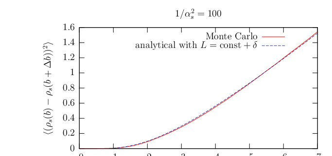
In order to check these expressions, we performed numerical simulations of models which possess the main characteristics of the QCD evolution while being simple enough to allow for robust Monte Carlo simulations (see Ref. [6] for details). We found a perfect matching with the parameter-free analytical result (3) in the limit $\log(1/\alpha_{s}^{2})\gg 1$. For larger and more realistic values of $\alpha_{s}$, the persistence of the correlations is still seen in the numerical simulations, but some parameters should be modified in the analytical expressions and tuned to account for our lack of understanding of subleading corrections important for finite $\log(1/\alpha_{s}^{2})$. We show such a calculation for $\alpha_{s}=0.1$ in Fig. 3, compared to a variant of Eq. (3).

The main result of our work is that the characteristic distance of the correlations in the transverse plane is not $1/Q_{s}$ as one would naively expect, but rather $\exp\left[c\log^{2}(1/\alpha_{s}^{2})\right]/Q_{s}$ ($c$ being a known constant), which is parametrically much larger than $1/Q_{s}$. Our results are valid for large $\log(1/\alpha_{s}^{2})$, and for distances $\Delta b$ much smaller than the typical confinement scale $1/\Lambda_{\mbox{\small QCD}}$.

The goal of our work was to understand the fundamentals of the QCD dynamics in transverse space, without thinking a priori of any application to phenomenology. Let us however note that recently, a diffractive deep-inelastic scattering observable was proposed that would directly probe the correlations which we have computed [7]. (A calculation of these correlations in the framework of the B-JIMWLK formalism [1] which a priori neglects the fluctuations discussed in this paper was also performed.) Also, these correlations may play an important role in heavy-ion collisions.

References

- [1] F. Gelis, E. Iancu, J. Jalilian-Marian and R. Venugopalan, arXiv:1002.0333 [hep-ph].
- [2] K. J. Golec-Biernat, M. Wüsthoff, Phys. Rev. D59 (1999) 014017.
- [3] S. Munier, Phys. Rept. 473 (2009) 1.
- [4] S. Munier, G. P. Salam, G. Soyez, Phys. Rev. D78 (2008) 054009.
- [5] E. Brunet, B. Derrida, A. H. Mueller and S. Munier, Phys. Rev. E73 (2006) 056126.
- [6] A. H. Mueller and S. Munier, Phys. Rev. D81 (2010) 105014.
- [7] C. Marquet and H. Weigert, arXiv:1003.0813 [hep-ph].