Step-scaling with off-shell renormalisation

In the original RI/MOM kinematic choice a single gluon can carry all the hard momentum through the vertex leading to infra-red effects which fall only as $\frac{1}{p^{2}}$. Depending on the operator these effects have a non-trivial dependence on the valence quark mass that can complicate mass extrapolations, and in some cases require pion pole subtraction [1, 5, 6, 7].

RBC and UKQCD have developed the non-exceptional momentum, SMOM, kinematic point as a preferred matching condition [8]. A significant gain comes from the extra suppression of non-perturbative effects. The perturbative expansion must be calculated for non-exceptional momenta; this has been performed to one loop for bilinear operators [9] and for $B_{K}$ [10]. Two recent publications have extended this to two loops for two different schemes for the quark mass [12, 11]. The non-exceptional kinematic point for bilinears has

$$p_{1}^{2}=p_{2}^{2}=(p_{1}-p_{2})^{2}.$$

(4)

RBC and UKQCD have found [8] that both momentum and mass dependence are simplified with non-exceptional kinematics. With this momentum flow, multiple hard gluons are required to create a soft sub-graph and non-perturbative infra-red effects, such as spontaneous chiral symmetry breaking, fall as a higher power of the external momentum, $\frac{1}{p^{6}}$ [13]. As our aim is to carefully study vertex functions while reducing the volume, we require a momentum scheme that is not sensitive to condensate physics.

The original method used a single point source to calculate momentum space Green’s functions. The volume source technique was developed by QCDSF [2]. The attraction here is to evaluate the amputated vertex function with the operator insertion averaged over all $L^{4}$ lattice sites. We shall see it is easily possible to obtain 0.1% statistical errors with volume source techniques, and even smaller if hundreds of configurations or larger volumes were used. With this statistical precision systematic effects like ${\cal{O}}(4)$ breaking lattice artefacts are visible and are in fact the dominant systematic error. These must either be included in the error analysis or better yet addressed using the techniques of this paper to escape the Fourier constraints.

We use $i$, $j$ to represent colour indices, and $\alpha$, $\beta$ to represent spin indices. We define the four momentum source, used on a Landau gauge fixed configuration, as

$$\eta_{p}(x)=e^{ip_{\mu}x^{\mu}}\delta_{ij}\delta_{\alpha\beta},$$

(5)

where the (dimensionless) momenta are $ap_{\mu}=n_{\mu}\frac{2\pi}{L_{\mu}}$. On a given gauge field $U_{\mu}(x)$ we solve

$$\sum_{x}D_{\rm dwf}(y,x)G(x,p)=\eta_{p}(y),$$

(6)

and $D_{\rm dwf}$ is the Domain Wall fermion matrix [3]. One propagator inversion for each leg momentum is necessary, but this cost is more than offset by the gain in statistical accuracy from the volume average.

To compute the external legs required for amputating the vertex functions we require the momentum space propagator

$$G(p_{1},p_{1})=\sum\limits_{x}e^{-ip_{1}^{\mu}x_{\mu}}G(x,p_{1}).$$

(7)

We form phased propagators for each momentum:

$$G^{\prime}(x,p)=G(x,p)e^{-ip\cdot x}=\sum_{y}D_{\rm dwf}^{-1}(x,y)e^{ip\cdot(y-x)}.$$

(8)

We select two independent momenta $p_{1}$, and $p_{2}$, and form unamputated bilinear vertex functions $V_{\Gamma}$ for Dirac structure $\Gamma$:

$$V_{\Gamma}^{\text{bilinear}}(p_{1},p_{2})=\left[\sum_{x}\gamma_{5}(G^{\prime}(x,p_{1}))^{\dagger}\gamma_{5}\Gamma G^{\prime}(x,p_{2})\right]_{ij,\alpha\beta},$$

(9)

and also for four quark operators:

$$V_{\Gamma\Gamma}^{\text{4q}}(p_{1},p_{2})=\sum_{x}\left(\gamma_{5}(G^{\prime}(x,p_{1}))^{\dagger}\gamma_{5}\Gamma G^{\prime}(x,p_{2})\right)_{ij,\alpha\beta}\left(\gamma_{5}(G^{\prime}(x,p_{1}))^{\dagger}\gamma_{5}\Gamma G^{\prime}(x,p_{2})\right)_{kl,\gamma\delta}.$$

(10)

Here, external colour and spin indices are left free for off line amputation and projection. This allows us to define the amputated Green’s function as, for example,

$$\Pi_{\Gamma}(p)=\left(G^{-1}(p_{1},p_{1})V_{\Gamma}(p_{1},p_{2})\gamma_{5}[G^{-1}(p_{2},p_{2})]^{\dagger}\gamma_{5}\right)$$

(11)

where $p^{2}=p_{1}^{2}=p_{2}^{2}=(p_{1}-p_{2})^{2}$, and we take $q=p_{1}-p_{2}$. The bare vertex amplitudes are then obtained by projecting the amputated Green’s functions onto their tree level values, for example

$$\Lambda_{\Gamma}=\frac{1}{12}Tr\left(\Pi_{\Gamma}\Gamma\right).$$

(12)

In continuum Euclidean space simultaneously rotating all momenta in a scattering amplitude by any $O(4)$ matrix must give equivalent results. However, in our discrete system there is only $H(4)$ symmetry and, even in the infinite volume, only momenta related by $\pi/2$ rotations and reflections are equivalent. Vertex functions will receive different $O(a^{2})$ errors depending on the direction of the momentum relative to the lattice axes. The original studies did not resolve ${\cal O}(4)$ breaking lattice artefacts due to statistical imprecision. Different ${\cal O}(4)$ equivalent but ${\cal H}(4)$ distinct momentum configurations, given by different Fourier modes, were treated interchangeably and simply averaged together. This is backed to some extent by the Rome-Southampton window argument for a region of safe operation with respect to lattice artefacts.

When the method outlined above is combined with a continuum extrapolation, the naive use of ${\cal H}(4)$ inequivalent momenta as interchangeable is theoretically unsound because $O(4)$ breaking is a component of the lattice artefacts that should be removed by the extrapolation. If the orientation of momenta relative to lattice axes does not remain fixed as $a$ is changed, an extrapolation in $a$ is not formally valid as one uses a different observable for each lattice spacing (differing due to ${\cal H}(4)$ inequivalent momentum choices). The Fourier constraints make it difficult to select the same physical momentum simultaneously on more than one lattice spacing, and these differing $O(4)$ breaking lattice artefacts necessarily enter each data point in a continuum extrapolation of data renormalised using the Rome-Southampton method. This introduces an intrinsic systematic uncertainty at a level set by the size of $O(4)$ breaking artefacts.

$O(4)$ breaking effects were argued to be ignorable as they were not statistically resolved. This justifies smooth interpolation in $p^{2}$ to obtain matched physical momenta.

It also somewhat justifies an (otherwise dubious) continuum extrapolation. We measure the vertex function observable on different lattice spacings at the same physical momentum magnitude, but must pick ${\cal H}(4)$ inequivalent momenta to satisfy Fourier constraints. This results in incorrectly parametrised lattice artefacts, however ${\cal O}(4)$ breaking effects can be safely ignored when they are substantially smaller than statistical errors.

With the volume source technique, however, $O(4)$ breaking effects are well resolved and are a dominant systematic error. This compromises our ability to perform a continuum extrapolation, and these considerations represent a serious problem that we address in this paper with the use of twisted boundary conditions.

From the discussion of the previous subsection III.1 we see that it would be rather better to crisply remove lattice artefacts by continuum extrapolation, and only apply perturbative matching in the continuum limit. This is difficult when constrained to use Fourier modes. Applying twisted boundary conditions to propagator inversions enables arbitrary momenta to be used. The twisted boundary approach differs by only finite volume effects from a simulation on a much larger lattice with an exact Fourier mode of the same momentum.

In order to simultaneously satisfy the constraint (4) and only use one momentum direction we propose choosing one kinematic satisfying (4) and use twisted boundary conditions [25, 26, 27, 29, 30], to vary the magnitude of the momentum. The twisting technique has been used to insert arbitrary three-momenta in form factor calculations with the success demonstrated, for example, by the direct comparison of refs [31, 32] to refs [30, 33, 34]. which make use of the same configurations and action.

In this paper the technique is used to allow arbitrary four-momenta to be used [25], and hence allow to rigorously disentangle discretisation and perturbative truncation effects for the first time. Of course, the lattice artefacts are still present at finite lattice spacing but, up to finite volume effects, these become the same lattice artefact at each lattice spacing. This is not the case if different Fourier modes are used. The goal is to enable us to determine the non-perturbative anomalous running in the RI scheme in the continuum limit prior to the use of continuum perturbation theory.

We now formulate the momentum space propagator calculation with twisted boundary conditions for use in off-shell renormalisation. Let the quark fields satisfy twisted boundary conditions $q(x+L)=e^{i\theta}q(x)$ and define [28]

$$\tilde{q}(x)=e^{-iBx}q(x)$$

(13)

with $aB_{\mu}=\frac{\theta}{L_{\mu}}$ so that $\tilde{q}(x)$ satisfies periodic boundary conditions. This transformation changes the continuum Dirac operator:

$$D=(\cancel{\partial}+m)\rightarrow\tilde{D}=(\cancel{\partial}+i\cancel{B}+m)$$

(14)

$\tilde{D}$ has inverse $\tilde{G}$ and $D$ has inverse $G$; they are related by

$$G(x,y)=e^{iB(x-y)}\tilde{G}(x,y)$$

(15)

using translational invariance which we should recover after gauge averaging. Let

$$\tilde{G}(z,p)=\sum_{x}\tilde{G}(z,x)e^{ipx}$$

(16)

then

$$\sum_{z}\tilde{D}(y,z)\tilde{G}(z,p)=e^{ipy}$$

(17)

So inverting the twisted Dirac operator (14) with a momentum source gives $\tilde{G}(z,p)$. Note that $\tilde{G}(z,x)$ satisfies periodic boundary conditions so that in the source term, $e^{ipy}$, $ap_{\mu}=\frac{2\pi n_{\mu}}{L_{\mu}}$ is a Fourier mode. $\tilde{G}(z,p)$ is related to $G(z,p)$ via,

$$\tilde{G}(z,p)=\sum_{x}e^{-iB(z-x)}G(z,x)e^{ipx}=e^{-iBz}G(z,p+B).$$

(18)

The propagator can be obtained from,

$$\tilde{G}(p,p)=\sum_{z}e^{-ipz}\tilde{G}(z,p)=\sum_{z,x}e^{-i(p+B)(z-x)}G(z,x)=G(p+B,p+B)$$

(19)

Thus the net effect of twisted boundary conditions is to shift the momentum $p$ to $p+B$ where B is arbitrary. In order to compute the non-exceptional Green’s functions observe,

$$\tilde{V}_{\Gamma}(p_{1},p_{2})=\sum_{x,y,z}e^{-ip_{1}(x-z)}\tilde{G}(x,z)\Gamma e^{-ip_{2}(z-y)}\tilde{G}(z,y)=\sum_{z}\gamma_{5}e^{ip_{1}z}\tilde{G}(z,p_{1})^{\dagger}\gamma_{5}\Gamma e^{-ip_{2}z}\tilde{G}(z,p_{2})$$

(20)

Using the inverse of (18) $\tilde{G}_{\Gamma}(p_{1},p_{2})$ the vertex function is seen to be,

$$\tilde{V}_{\Gamma}(p_{1},p_{2})=\sum_{x,y}\gamma_{5}e^{i(p_{1}+B_{1})x}G(x,p_{1}+B_{1})^{\dagger}\gamma_{5}\Gamma e^{-i(p_{2}+B_{2})y}G(y,p_{2}+B_{2})=V_{\Gamma}(p_{1}+B_{1},p_{2}+B_{2})$$

(21)

We consider the values for $p_{1}$, $p_{2}$, $B_{1}$ and $B_{2}$ in the following subsection.

We select Euclidean momenta in the direction of $p_{1}=(-1,0,1,0)$ and $p_{2}=(0,1,1,0)$ up to $H(4)$ symmetry operations. This choice minimises $S^{4}=\sum_{i}p_{i}^{4}$ which we take as measure of discretization errors, subject to the constraint that $p_{1}$/$p_{2}$/$(p_{1}-p_{2})$ be $H(4)$ equivalent momenta. It is certainly possible to rotate some combination of $p_{x},p_{y},p_{z}$ into the temporal direction breaking this $H(4)$ equivalence, and this would form an interesting possibility to demonstrate universality of the continuum limit in a later work.

The non-exceptional $p_{1}$/$p_{2}$/$(p_{1}-p_{2})$ kinematics can be represented by an equilateral triangle in momentum space with vertices lying on the $p_{x},p_{y},p_{z}$ coordinate axes (figure 1). Continuous dilation of this triangle can be performed by using twisted boundary conditions with a fixed orientation of the $p_{1}$ , $p_{2}$, $p_{1}-p_{2}$ triangle. This continuity allows one to pick a fixed MOM observable as the lattice spacing is varied. In particular, we choose parallel twisting vectors in the directions $B_{1}=(-\theta,0,\theta,0)$ corresponding to $p_{1}$ and $B_{2}=(0,\theta,\theta,0)$ corresponding to $p_{2}$. We continuously vary $\theta$ to move the vertices of the triangle along the axes.

The non-exceptional momenta are chosen to have small discretisation errors by spreading the power across multiple coordinate axes. In general for any non-exceptional configuration there will be $O(a^{2})$ errors. For exceptional momentum amplitudes we take vertex functions with $p_{1}$ on both legs. As the direction is kept fixed the vertex function is a smooth function of $(ap)^{2}$ and interpolation in momentum is possible. Extrapolation to the continuum limit at fixed physical momentum is now theoretically justified.

Between different lattice spacings we compare only renormalised quantities and their ratios. This is quite natural as we desire to take the continuum limit of the product of a bare operator matrix element and its RI scheme renormalisation constant at some accessible scale $p$. The scaling factors for each operator to match between different $\beta$’s introduced in [23] are then not required. The aim of the latter part of this paper will be to raise, in the continuum limit, this scale $p$ to one ($s^{n}p$ where $s$ is a scale factor) where there is better perturbative convergence.

We eliminate $Z_{q}$ via the vertex function of the (conserved) vector or axial currents:

$$R_{\cal O}(p,a,m)=\frac{\Lambda_{A}(p,a,m)}{\Lambda_{\cal O}(p,a,m)}=\frac{Z_{\cal O}(p,a,m)}{Z_{A}}$$

(22)

and this ratio will be extrapolated to the chiral limit to produce a renormalization constant

$$Z_{\cal O}(a,p)=Z_{A}\lim_{m\to 0}R_{\cal O}(p,a,m)$$

(23)

where, for convenience, we use the vertex function of the local rather than conserved axial current and eliminate this with a previously computed $Z_{A}$. We then continuum extrapolate the product of $Z_{\cal O}$ with $\langle{\cal O}\rangle$:

$$\langle{\cal O}\rangle^{\rm ren}=\lim_{a\to 0}\langle{\cal O}\rangle Z_{{\cal O}}.$$

(24)

This gives $\langle\cal O\rangle$ in the RI/MOM scheme at a scale determined by the physical momentum chosen which must be the same scale on all the lattices used to take the continuum limit.

We also consider the factor required to convert $\langle{\cal O}\rangle$ at scale $p$ to scale $sp$ where $s>1$ is a scale factor. This is

$$\Sigma_{\cal O}(p,sp,a)=\lim_{m\to 0}\frac{R_{\cal O}(sp,a,m)}{R_{\cal O}(p,a,m)},$$

(25)

and its continuum limit is

$$\sigma_{\cal O}(p,sp)=\lim_{a\to 0}\Sigma_{\cal O}(p,sp,a).$$

(26)

$\sigma_{\cal O}(p,sp)$ encodes the scale dependence of the RI scheme in the continuum limit expanded around the scale $p$. We can then assess the degree to which the running around our match scale is perturbative without risk of confusion by possible lattice artefacts. By picking a well defined momentum orientation for the amplitude as a function of $a$, we remove the ambiguity in taking the continuum limit that arises when selecting different Fourier modes for each value of $\beta$.

We have demonstrated how to obtain a controlled expansion in powers of the lattice spacing for amputated vertex functions and gain better control of lattice artefacts via continuum extrapolation.

Step scaling has been well developed in the Schrödinger functional approach [15, 14, 16, 17, 18, 19, 20, 16]. A finite volume scheme based on Creutz ratios has also been recently developed [21]. In this paper we seek to develop a related approach based on the Landau gauge fixed RI/MOM method. Our approach does not tie the renormalisation scale to the volume, and therefore also avoids the need to fine tune bare couplings to precisely match a volume sensitive renormalised coupling between simulations.

After reviewing existing step scaling methods we will attempt to address perturbative errors associated with the low-end of the Rome-Southampton scaling window by raising the scale at which we match to perturbation theory by introducing a new step scaling scheme. In order to use the same notational conventions as the literature on step scaling in the Schrödinger functional scheme, for the rest of this section let $L$ represent the length of the lattice in physical units rather than units of lattice spacing. This departs from our convention elsewhere in the paper, which takes $L$ as an integer lattice size and is consistent with notation typically used for RI/MOM renormalization.

In order to develop a practical step scaling scheme we require several pieces. Firstly, we have defined continuum limit non-perturbative evolution ratios that can be used to access higher momentum scales. Step scaling will combine a sequence of these objects, each determined inexpensively compared with a brute force method.

We believe that three technical advantages we have over the earlier attempt at RI/MOM step scaling make the task more tractable. The first, volume sources, reduces statistical errors greatly giving precision to the approach. The second, non-exceptional momenta, renders mass dependence and infra-red behaviour in $p^{2}$ benign; this greatly assists with both chiral extrapolation and matching between ensembles, in addition to finite volume sensitivity. These were described above.

In this paper we have introduced a third advantage: using twisted boundary conditions to select arbitrary four momenta. The direction of the scattering momenta can be kept fixed relative to lattice axes and arbitrary values of $p^{2}$ can be chosen. This is a Good Thing because it allows the same physical momenta according to the lattice symmetries $H(4)$ to be chosen on each ensemble. The vertex function observable will only then have a valid expansion in powers of the lattice spacing $a$. This approach enables precise matching of momenta between ensembles, and precise continuum extrapolation.

We will keep the off-shell momentum scales hard enough that the physical volume should not be resolved. In this way the the calculation will be finite volume effect safe, and the perturbative matching will use the standard infinite volume perturbation theory already available to high order for off-shell renormalisation. These are significant advantages over the Schrödinger functional.

For the scheme to be affordable it is therefore necessary that it be able to operate in a small physical volume. For offshell amplitudes this is the case whenever the virtuality is too hard to resolve the finite volume

$$p^{2}\gg(\frac{\pi}{L})^{2}.$$

(27)

Thus, for the purposes of step scaling, the window condition Eq (1) becomes

$$(\frac{\pi}{L})^{2}\ll p^{2}\ll\left(\frac{\pi}{a}\right)^{2}.$$

(28)

This latter condition is likely possible to meet using modest lattice volumes $\frac{L}{a}\leq 16$ at all stages of the calculation. We will compute vertex functions on lattices at different values of $\beta$ with overlapping scaling windows. This will then enable the determination of a continuum step scaling function for some operator ${\cal O}$ at a physical scale $p^{2}$ chosen in the window Eq (28) to that at a scale larger by a scale factor $s$. This is precisely $\sigma_{\cal O}(p,sp)$ from the previous section.

These can be combined in a series of non-perturbative steps to a high scale, with perturbative conversion to $\overline{MS}$ is then applied only where it is well convergent. For example,

$$\begin{array}[]{ccc}\langle{\cal O}^{\overline{MS}}(\mu)\rangle&=&\langle{\cal O}^{\rm SMOM}(p)\rangle\\ &\times&\sigma^{1}_{\cal O}(p,sp)\\ &\times&\sigma^{2}_{\cal O}(sp,s^{2}p)\\ &\ldots&\\ &\times&\sigma^{n}_{\cal O}(s^{n-1}p,s^{n}p)\\ &\times&\left[1+c^{\rm SMOM\to\overline{MS}}\alpha_{s}(\mu=s^{n}p)\right].\end{array}$$

(29)

It appears clear that Eq (28) can be satisfied at reasonable expense. For example $16^{3}$ domain wall fermion simulations will be inexpensive with the next generation of supercomputers; multiple such ensembles dedicated solely to the renormalisation of lattice operators are quite affordable. This is particularly helped by the relatively benign mass dependence of non-exceptional momentum vertex functions. It is also clear that on these proposed small ensembles all hadronic quantities must be avoided to ensure finite volume safety of the analysis. For the determination of $m_{\rm res}$, the PCAC is an operator relation and so it is immaterial whether a finite volume or a physical pionic state is used to determine the ratio. Determining the lattice spacing (or more specifically the ratio of the lattice spacing to that of an earlier larger volume simulation) in a finite volume safe manner is discussed below.

In this section we focus on the data obtained using the $\beta=2.13$ ensembles and display the quality of data obtained on a single lattice spacing.

Figure 2 contains a comparison of the traditional volume averaged Fourier mode NPR to our new twisted boundary condition technique. We show the vector and axial vertex functions at fixed quark mass, $m_{q}=0.03$, and with exceptional momentum kinematics on the $\beta=2.13$ lattice, using 10 configurations. $O(4)$ breaking lattice artefacts produce a large scatter in the data using the traditional approach and this is scatter completely removed by the twisted boundary conditions technique. Of course, lattice artefacts are still present and of the same size, but the key point is that we can now vary $\beta$ while looking at the same off-shell momentum in order to extrapolate these away in the continuum limit.

For the exceptional kinematic configuration we use the projectors of [8] and the perturbative running and matching calculated in [42] for mass and [43] for the tensor current. For ${\cal O}_{VV+AA}$ we use the results of [44, 45]. We denote these exceptional momentum schemes RIMOM.

For non-exceptional kinematics we compare the two schemes introduced in [9]. The first is the scheme of [9] which corresponds to choosing projectors $\cancel{q}q_{\mu}$ for the vector vertex function and $\cancel{q}q_{\mu}\gamma_{5}$ for the axial vertex function. We denote this scheme SMOM-$\cancel{q}$. The second uses $\gamma_{\mu}$ and $\gamma_{\mu}\gamma_{5}$ for vector and axial vertex functions, we refer to this scheme as SMOM-$\gamma_{\mu}$. The one-loop matching and two-loop anomalous dimensions for tensor current and mass are given in [9]. These results have recently been extended to two loop matching and three loop anomalous dimensions [11, 12]. For ${\cal O}_{VV+AA}$ we use several unpublished new schemes and perturbative results by Sachrajda and Sturm [10], and we thank them for their private communications.

Figure 3 displays the vertex functions of all the operators analysed in this paper (bilinear Vector, Axial Vector, Scalar, Pseudoscalar, Tensor and four quark operator ${\cal O}_{VV+AA}$) for the $\beta=2.13$ ensemble, for both non-exceptional and exceptional momenta. We will return study each of these structures in turn and in more detail below.

We wish to eliminate the wavefunction renormalisation by taking ratios $\frac{\Lambda_{A}}{\Lambda_{O}}$ and where $\Lambda_{A}$ is the vertex function of the local axial current, and its renormalisation is eliminated using $Z_{A}$ previously determined from the ratio of matrix elements the local axial current and the conserved axial current From the Ward identities in the limit of small mass and large momentum we should find that $Z_{V}\simeq Z_{A}$ and $Z_{S}=Z_{P}$. These are well supported by our data for non-exceptional momentum but, over our momentum range, not held for exceptional momentum. In order to compare with previous results we adopt, for exceptional momentum, the the strategy of [8] eliminating the quark field renormalisation using

$$\frac{Z_{q}}{Z_{A}}=\frac{1}{2}(\Lambda_{A}+\Lambda_{V}),$$

(34)

where factors of $Z_{A}$ are then multiplied out using a previously calculated value. For exceptional data this matches central value conventions with [8]. The 2% difference between $\frac{1}{2}(\Lambda_{A}+\Lambda_{V})$ and $\Lambda_{A}$ is a chiral symmetry breaking uncertainty that propagates globally in operator renormalisation analysis as a systematic uncertainty (and is doubled for four quark operators). This uncertainty is eliminated for the non-exceptional momentum kinematic 4.

For the non-exceptional case we use simply $\frac{Z_{q}}{Z_{A}}=\Lambda_{A}$. In this case, we have

	$\displaystyle{Z_{m}Z_{A}}$	$\displaystyle=$	$\displaystyle\frac{\Lambda_{S}}{\Lambda_{A}},$		(35)
	$\displaystyle\frac{Z_{T}}{Z_{A}}$	$\displaystyle=$	$\displaystyle\frac{\Lambda_{A}}{\Lambda_{T}},$		(36)
	$\displaystyle Z_{B_{K}}=\frac{Z_{{\cal O}_{VV+AA}}}{Z_{A}^{2}}$	$\displaystyle=$	$\displaystyle\frac{\Lambda_{A}^{2}}{\Lambda_{{\cal O}_{VV+AA}}}.$		(37)

Our results for RIMOM, SMOM-$\cancel{q}$, and SMOM-$\gamma_{\mu}$ schemes for the wave function renormalisation determined from the axial current vertex function (non-exceptional) and average of axial and vector vertex functions (exceptional) are displayed in figure 5. Here, the running at this lattice spacing is poorly described by continuum perturbation theory, and is associated with the momentum dependence of the exponent for binding of light modes in the fifth dimension in the domain wall formulation [46]. We note that this $Z_{q}$ is cancelled in the ratios above when treating other operators. Naturally, one expects that such discretisation effects will be removed if a controlled continuum limit is taken, and this will be revisited in later sections.

Figures 6, 7, and 8 display the corresponding data for the mass, tensor current and four quark operator ${\cal O}_{VV+AA}$ relevant for $B_{K}$. As promised, the data is extremely precise and ${\cal O}(4)$ breaking discretisation effects do not introduce scatter in the data as the momentum is changed because we are always selecting the same lattice momentum with our twisted boundary conditions. Errors are at the 0.1% level even on this relatively small volume and with only twenty configurations.

In contrast to $Z_{q}$, the running of $Z_{m}$, $Z_{T}$, and $Z_{VV+AA}$ is reasonably well described by continuum perturbation theory for larger values of $p^{2}$, even on this non-zero lattice spacing. This is indicated by reduction of the slope of the data after perturbative conversion to $\overline{MS}$ (blue) especially at higher momenta. Residual $p^{2}$ dependence remains after this conversion at the few percent scale. This reflects an admixture of lattice artefacts, and perturbative truncation error. The methods introduced in this paper enable the continuum limit of the scale evolution to be determined and disentangle these sources of error.

Table 4 shows our results compared with the results of Ref [8] after following the same procedure of converting to the $\overline{MS}$ scheme at 2 GeV and then extrapolating to $p^{2}=0$. In all cases the extrapolation was performed using a linear fit of $\Lambda_{O}$ as a function of $(ap)^{2}$ in the range $2<(ap)^{2}<3.2$. This procedure is flawed. We note that this is in danger of extrapolating perturbative errors into the infrared. In the next section we show instead how to take the continuum limit at non-zero momentum to eliminate discretisation errors. These numbers are thus for comparison only, and constitute a check and a demonstration of the precision that is possible using the techniques of this paper. The numbers do not represent an attempt to improve on previous estimates of renormalization constants for the RBC-UKQCD domain wall programme. The physical RBC-UKQCD predictions will be updated using the methods of this paper techniques in later works, where we will also use step scaling to raise the momentum scale to minimise perturbative error.

Determining the lattice spacing for our $\beta=2.23$ ensemble is a useful test case for the methods of section IV.2.1. As a preliminary we have calculated $r_{C}$ for our $16^{3}$ lattices. We compute timelike Wilson loops with four hits of APE smearing, smearing parameter 2.5, in the spatial direction. The tree level improvement of [35] is here required for the Iwasaki gluon action. We compute the tree level Wilson loop using code developed in [47] to obtain Table 6 where the potential includes the self energy part.

$$aV(\vec{R}a)=-\lim_{T\to\infty}\frac{1}{W(\vec{R},T)}\frac{dW(\vec{R},T)}{dT}=C_{F}V(\vec{R})g^{2}+O(g^{4})$$

(38)

By demanding

$$F(r_{I})=(V(r)-V(r-a))/a=F_{tree}=\frac{1}{4\pi r_{I}^{2}}$$

(39)

we solve for $r_{I}$ using Table 6. This approach leads to much reduced lattice $O(a^{2})$ errors [35] [48]. Further, using the force instead of the potential removes the self energy part and reduces the linear term, $\sigma r$, to a constant. Fitting the Cornell potential to find $r_{C}$ requires $\sigma$. However, $\sigma$ is dependant on the long distance behaviour of $V(r)$, and to constrain it one has to sample large $r$. When fitting to the force, $r_{C}$ can be obtained without including large distance data in the procedure, and $r_{C}$ computed this way is a finite volume safe observable with which to determine the lattice spacing.

In order to extract $V(r)$ from the average Wilson loops $\langle W(r,t)\rangle$ we first plot the effective potential

$$\log(\frac{\langle W(r,t+1)\rangle}{\langle W(r,t)\rangle})$$

(40)

as a function of $t$. The largest value of $r$ used in this analysis is $4a$. Excited state contamination and statistical noise are problematic, and we use the ’black box’ method [49] to define an improved effective mass that takes account of the first excited state. This allows us to extend $t_{min}$ to $t=3$ which gives a significant error reduction compared to the usual effective mass. On the $\beta=2.13$ lattice we use $600$ configurations for each mass, each configuration rotated to use 4 different time directions. For $\beta=2.23$ we use $750$ configurations per mass and again rotate the time direction.

The equation $r^{2}F(r)=C$ has solutions in the range of our data for $C\in(0.6,2.0)$. Lower values give more accurate $r_{C}$ but these are likely to have large discretisation errors. For any $C$ however $\frac{r_{C}/a_{2.13}}{r_{C}/a_{2.23}}$ should be constant, we plot this ratio as a function of $C$ in figure 10 and determine $C>1.4$ is appropriate and gives the value for the ratio of lattice scales,

$$R_{a}^{2}=\frac{(a_{2.23})^{2}}{(a_{2.13})^{2}}=0.652(21)$$

(41)

This implies a lattice spacing of $a^{-1}\simeq 2.14$ GeV for the $\beta=2.23$ ensembles.

We propose below a scale factor $s=1.5$, and believe that at least two iterations of step scaling should be possible based only on the static potential. However, the static potential displays percent scale errors even with many configurations and finding a more precise alternative would certainly be good in any case.

Following equation 26 we can compute $\sigma_{O}(p,sp)$ using two lattice spacings. We consider the evolution of renormalisation constants $Z_{q}$, $Z_{m}$, $Z_{T}$, and $Z_{B_{K}}$ in both the exceptional and the non-exceptional kinematic schemes. We choose $p\simeq 2(GeV)$ and compute $\sigma_{O}(p,sp)$ as a function of s.

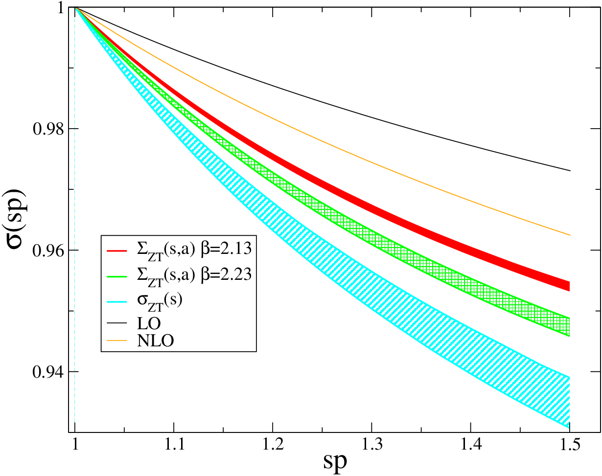
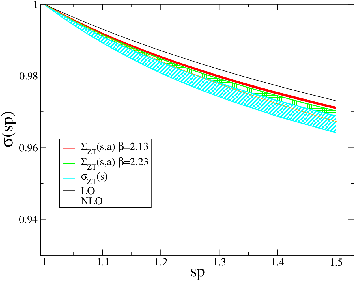
Because of the very smooth $p^{2}$ dependence of the vertex functions computed with twisted boundary conditions we can perform a simple interpolation to match values of $p^{2}$ on each lattice. One could in principle simulate at the same physical momentum on each lattice by choosing the twisting angles appropriately, however since the interpolation introduced only a very small uncertainty this was not necessary.

For each operator we can now evaluate $\Sigma_{O}(p=2{\rm GeV},sp,a^{-1}=1.729{\rm GeV})$ and $\Sigma_{O}(p=2{\rm GeV},sp,a^{-1}=2.14{\rm GeV})$. Linear extrapolation in $a^{2}$ with only two datapoints is not as robust as one might like, but certainly suffices to demonstrate the method. Using this, we can obtain the continuum limit step scaling function $\sigma_{O}(p=2{\rm GeV},sp)$ for the quark field (figure 11), mass (figure 12), tensor current (figure 13), and the four quark operator ${\cal O}_{VV+AA}$ (figure 14). With an appropriate third and smaller lattice spacing using a correspondingly smaller volume we could similarly determine the next step, evolving from 3 GeV to 4.5 GeV and so on.

Figure 11 is especially important, because $Z_{q}$ suffers from the greatest lattice artefacts for Domain Wall Fermions, and is carefully eliminated in the NPR analysis of other operators.

In the $\gamma_{\mu}$ scheme, with both exceptional and non-exceptional momenta, the finite lattice spacing running of $Z_{q}$ is in the opposite direction to the perturbative prediction, however the running behaviour recovered in the continuum limit is close to perturbative. The determination of $Z_{q}$ with domain wall fermions displays the momentum dependence of the exponent, $\alpha(p)$, of localisation in the fifth dimension [46]. As shown here, in a number of schemes, as long as an unambiguous continuum limit can be defined, the Domain-Wall action will then produce the continuum scaling behaviour of $Z_{q}$ and the other renormalization constants.

References

- [1] G. Martinelli, C. Pittori, C. T. Sachrajda, M. Testa and A. Vladikas, Nucl. Phys. B 445 (1995) 81 [arXiv:hep-lat/9411010].
- [2] M. Gockeler et al., Nucl. Phys. B 544 (1999) 699 [arXiv:hep-lat/9807044].
- [3] V. Furman and Y. Shamir, Nucl. Phys. B 439 (1995) 54 [arXiv:hep-lat/9405004].
- [4] Y. Iwasaki, Nucl. Phys. B 258 (1985) 141.
- [5] T. Blum et al., Phys. Rev. D 66 (2002) 014504 [arXiv:hep-lat/0102005].
- [6] H. D. Politzer, Nucl. Phys. B 117 (1976) 397.
- [7] P. Pascual and E. de Rafael, Z. Phys. C 12 (1982) 127.
- [8] Y. Aoki et al., Phys. Rev. D 78 (2008) 054510 [arXiv:0712.1061 [hep-lat]].
- [9] C. Sturm, Y. Aoki, N. H. Christ, T. Izubuchi, C. T. C. Sachrajda and A. Soni, Phys. Rev. D 80 (2009) 014501 [arXiv:0901.2599 [hep-ph]].
- [10] RBC and UKQCD collaboration “Continuum limit of from 2+1 Flavor Domain Wall QCD”, in preparation.
- [11] L. G. Almeida and C. Sturm, arXiv:1004.4613 [Unknown].
- [12] M. Gorbahn and S. Jager, arXiv:1004.3997 [Unknown].
- [13] Y. Aoki, “Non-perturbative renormalization in Lattice QCD”, PoS(Lattice 2009)012.
- [14] M. Luscher, R. Sommer, P. Weisz and U. Wolff, Nucl. Phys. B 413 (1994) 481 [arXiv:hep-lat/9309005].
- [15] M. Luscher, P. Weisz and U. Wolff, Nucl. Phys. B 359, 221 (1991).
- [16] A. Bode et al. [ALPHA Collaboration], Phys. Lett. B 515 (2001) 49 [arXiv:hep-lat/0105003].
- [17] S. Sint, Nucl. Phys. B 451 (1995) 416 [arXiv:hep-lat/9504005].
- [18] S. Sint, Nucl. Phys. Proc. Suppl. 42 (1995) 835 [arXiv:hep-lat/9411063].
- [19] M. Luscher, R. Sommer, U. Wolff and P. Weisz, Nucl. Phys. B 389 (1993) 247 [arXiv:hep-lat/9207010].
- [20] M. Luscher, R. Narayanan, P. Weisz and U. Wolff, Nucl. Phys. B 384 (1992) 168 [arXiv:hep-lat/9207009].
- [21] E. Bilgici et al., Phys. Rev. D 80 (2009) 034507 [arXiv:0902.3768 [hep-lat]].
- [22] Y. G. Zhestkov, PhD Thesis
- [23] Y. Zhestkov, arXiv:hep-lat/0101008.
- [24] K. Jansen et al., Phys. Lett. B 372 (1996) 275 [arXiv:hep-lat/9512009].
- [25] P. A. Boyle, Nucl. Phys. Proc. Suppl. 129 (2004) 358 [arXiv:hep-lat/0309100].
- [26] P. F. Bedaque, Phys. Lett. B 593 (2004) 82 [arXiv:nucl-th/0402051].
- [27] G. M. de Divitiis, R. Petronzio and N. Tantalo, Phys. Lett. B 595 (2004) 408 [arXiv:hep-lat/0405002].
- [28] C. T. Sachrajda and G. Villadoro, Phys. Lett. B 609 (2005) 73 [arXiv:hep-lat/0411033].
- [29] J. M. Flynn, A. Juttner and C. T. Sachrajda [UKQCD Collaboration], Phys. Lett. B 632 (2006) 313 [arXiv:hep-lat/0506016].
- [30] P. A. Boyle, J. M. Flynn, A. Juttner, C. T. Sachrajda and J. M. Zanotti, JHEP 0705 (2007) 016 [arXiv:hep-lat/0703005].
- [31] P. A. Boyle et al., Phys. Rev. Lett. 100 (2008) 141601 [arXiv:0710.5136 [hep-lat]].
- [32] D. J. Antonio et al., arXiv:hep-lat/0702026.
- [33] P. A. Boyle et al., JHEP 0807 (2008) 112 [arXiv:0804.3971 [hep-lat]].
- [34] P. A. Boyle et al., arXiv:1004.0886 [Unknown].
- [35] S. Necco and R. Sommer, Nucl. Phys. B 622 (2002) 328 [arXiv:hep-lat/0108008].
- [36] R. Sommer, Nucl. Phys. B 411 (1994) 839 [arXiv:hep-lat/9310022].
- [37] C. Allton et al. [RBC and UKQCD Collaborations], Phys. Rev. D 76 (2007) 014504 [arXiv:hep-lat/0701013].
- [38] D. J. Antonio et al. [RBC and UKQCD Collaborations], Phys. Rev. D 75 (2007) 114501 [arXiv:hep-lat/0612005].
- [39] D. J. Antonio et al. [RBC Collaboration and UKQCD Collaboration], Phys. Rev. D 77 (2008) 014509 [arXiv:0705.2340 [hep-lat]].
- [40] RBC-UKQCD Collaboration, “Continuum Limit Physics from 2+1 Flavor Domain Wall QCD” In preparation
- [41] C. Allton et al. [RBC-UKQCD Collaboration], Phys. Rev. D 78 (2008) 114509 [arXiv:0804.0473 [hep-lat]].
- [42] K. G. Chetyrkin and A. Retey, Nucl. Phys. B 583, 3 (2000) [arXiv:hep-ph/9910332].
- [43] J. A. Gracey, Nucl. Phys. B 662 (2003) 247 [arXiv:hep-ph/0304113].
- [44] A. J. Buras, M. Misiak and J. Urban, Nucl. Phys. B 586 (2000) 397 [arXiv:hep-ph/0005183].
- [45] M. Ciuchini, E. Franco, V. Lubicz, G. Martinelli, I. Scimemi and L. Silvestrini, Nucl. Phys. B 523 (1998) 501 [arXiv:hep-ph/9711402].
- [46] Y. Shamir, Nucl. Phys. B 406 (1993) 90 [arXiv:hep-lat/9303005].
- [47] G. S. Bali and P. Boyle, arXiv:hep-lat/0210033.
- [48] A. Hasenfratz, R. Hoffmann and F. Knechtli, Nucl. Phys. Proc. Suppl. 106 (2002) 418 [arXiv:hep-lat/0110168].
- [49] G. T. Fleming, arXiv:hep-lat/0403023.
- [50] P. A. Boyle, “The BAGEL assembler generator”, Computer Physics Communications 180/12:2739 (2009) [doi:10.1016/j.cpc.2009.08.010]