Magnetar Oscillations I: strongly coupled dynamics of the crust and the core

In this subsection we explore the behavior of this system by direct numerical simulations. We found this to be helpful in the building of our intuition. We defer a semi-analytical normal-mode analysis to the next subsection.

We follow L07 and for concreteness concentrate on a specific example; it will be clear that the conclusions we reach are general. We choose $\omega_{0}=1$rad/second and mass $M=1$. We choose a total number of 1000 small pendulae with frequencies $\omega_{n}=(0.5+n/1000)$rad/second and masses $m_{n}=m=10^{-4}$, to mimic the continuum frequency range between $0.5$rad/second and $1.5$rad/second. The simulation is initiated by displacing the large oscillator while keeping the small pendulae relaxed (this mimics the stresses in the crust), and then releasing. The subsequent motion of the system is then followed numerically by using a second order leapfrog integration scheme which conserves the energy with high precision. The resulting motion of the large pendulum can be decomposed into three stages (see Fig. 2 and Fig. 3):

(1) During the first 50-60 seconds, there is a rapid exponential decay of the large oscillator’s motion, during which most of the energy is transferred to the multitude (i.e., the ’continuum’) of small oscillators. This is the so-called phenomenon of “resonant absorption”, which has been studied for decades in the MHD and plasma physics community (e.g., Ionson 1978, Hollweg 1987, Goedbloed & Poedts 2004, L07, Gruzinov 2008b). In this first stage, the amplitude of the big pendulum motions drops by a factor of $\sim 100$.

(2) After $\sim 60$ seconds, the exponential decay stops abruptly as the large oscillator now reacts to the collective pull of the small ones. This second stage is characterized by a slow algebraic decay of the amplitude of the big pendulum displacement. Gruzinov (2008b) explains this as being due to the branch cut in the oscillator’s response function.

(3) The motion of the large oscillator stabilizes at a constant level (L07 missed this stage in his simulations, which he stopped too early). Fourier transform reveals 2 QPOs at the frequencies close to the continuum edges, $\omega=0.5$ and $\omega=1.5$; the same QPO frequencies can be observed in the previous stage (2) as well.

What is the origin of the QPOs, and how is this eventual stability established? In Fig. 4 and 5, we show how the amplitude of the small oscillators evolves with time.

After the initial resonant absorption phase, the amplitude is distributed as a Lorentzian centered on the frequency around $\omega=1$; this is because the small oscillators in resonance with the large one are the ones which gain the most energy. However, in subsequent times we see that the energy exchange occurs between the small oscillators³³ 3 This is much akin to the well-known phenomenon of resonant energy exchange between 2 equal-frequency pendulae hanging on the same supporting wall., and that the net result of this exchange is the energy flow towards the oscillators whose frequencies are near the edges. By the time the third stage begins, the amplitudes of the oscillators near the edge stabilize and their phases become locked. They are pulling and pushing the large oscillator in unison. In the next subsection, we show that this behavior is due to the presence of the edge normal modes, and we shall derive their frequencies and amplitudes.

In this section we deal with the system of coupled harmonic oscillators, and one should be able to find its normal modes using the standard techniques (Landau and Lifshitz mechanics, §23). However, the fact that all small oscillators are attached to the large one, and there is no direct coupling between the small oscillators, allows us a significant shortcut (in Appendix A, we treat a more general problem of several large oscillators coupled to a multitude of the core modes). We proceed as follows:

Suppose that we impose on the large oscillator a periodic motion with angular frequency $\Omega$, by driving it externally with the force $F_{\rm ext}=F_{0}(\Omega)\exp(i\Omega t)$. This motion in turn drives the small oscillators according to Eq. (1):

$$\ddot{x}_{n}+\omega_{n}^{2}x_{n}=\Omega^{2}x_{0},$$

(3)

which has the steady state solution:

$$x_{n}=\frac{\Omega^{2}}{\omega_{n}^{2}-\Omega^{2}}x_{0}$$

(4)

where we have omitted the time dependent factor $\exp(i\Omega t)$ on both sides. The combined force $f_{\rm cont}$ of the small oscillators acting back on the large one (see Eq. (2)) is given by

$$f_{\rm cont}\left(\Omega\right)=\sum_{n}m_{n}\omega_{n}^{2}\frac{\Omega^{2}}{\omega_{n}^{2}-\Omega^{2}}x_{0}.$$

(5)

According to Newton’s second law,

$$F_{0}\left(\Omega\right)+f_{\rm cont}\left(\Omega\right)=-M(\Omega^{2}-\omega_{0}^{2})x_{0}.$$

(6)

If $\Omega$ corresponds to the normal-mode frequency, then $F_{0}(\Omega)=0$. Hence by substituting Eq. (5) into Eq. (6) we get the following eigenvalue equation for $\Omega$:

$$G(\Omega)=M\left(\omega_{0}^{2}-\Omega^{2}\right)-\sum_{n}m_{n}\omega_{n}^{2}\frac{\Omega^{2}}{\omega_{n}^{2}-\Omega^{2}}=0.$$

(7)

In the continuum limit $N\rightarrow\infty$, the above equation becomes

$$G(\Omega)=M\left(\omega_{0}^{2}-\Omega^{2}\right)-\int_{\omega_{\rm min}}^{\omega_{\rm max}}d\omega\rho(\omega)\omega^{2}\frac{\Omega^{2}}{\omega^{2}-\Omega^{2}}=0,$$

(8)

where $\rho(\omega)=dm/d\omega$ is the mass per unit frequency of the continuum modes.

In the discrete case, the solutions of Eq. (7) are $N-1$ frequencies $\Omega_{i}$ that are within the quasi-continuum ($\omega_{i}<\Omega_{i+1}<\omega_{i+1}$, for $i=1,2,...N-1$; ’quasi-continuum modes’), and $2$ modes with frequencies $\Omega_{\rm low}$ and $\Omega_{\rm high}$ (the ’edge-modes’) that are near the edges, but outside, of the continuum (i.e. $\Omega_{\rm low}<\omega_{1}$ and $\Omega_{\rm high}>\omega_{N}$). It can be shown from Eq. (7) that in the limit $N\gg 1$ and $m_{n}\ll M$, the contribution of the small oscillator to the $i$-th quasi-continuum mode is completely dominated by the pendulae that are in close resonance with the mode. More precisely, one can show that as the number of oscillators $N$ increases and $m_{n}$ decreases, the number of small oscillators contributing to the mode energy remains constant. However, for the two edge modes there is no such singular behavior in the limit of large $N$, and consequently they play a special role in the dynamics of the system.

This last point is clearly seen in the continuum case represented by Eq. (8). The eigenvalue equation has no real solutions in the range of small-oscillator continuum $\omega_{\rm min}<\Omega<\omega_{\rm max}$, since the response function $G(\Omega)$ is ill-defined in this interval⁴⁴ 4 There is a complex solution if the integration in the expression for $G(\Omega)$ is performed along the contour chosen according to the Landau rule. One then obtains a “resonantly absorbed” or “Landau-damped” mode (Gruzinov 2008b, L07), which exactly represents the exponential decay of stage (1) in our numerical experiment of the previous subsection.. However, the edge modes on both sides of the continuum interval remain, and their frequencies can be found by numerically evaluating the zero points of $G(\Omega)$ in Eq. (8). For the numerical of the previous subsection, one finds $\Omega_{\rm low}=0.5-8.2\cdotp 10^{-6}$ and $\Omega_{\rm high}=1.5+8.6\cdotp 10^{-4}$. Analytically, one can find the following scaling for the distance $\delta\omega_{\rm edge}$ between the mode frequency and the nearest edge $\omega_{\rm edge}$ of the continuum range:

$${\delta\omega_{\rm edge}\over\omega_{\rm edge}}=C\exp\left\{-{M|\Omega_{0}^{2}-\omega_{\rm edge}^{2}|\over\rho(\omega_{\rm edge})\omega_{\rm edge}^{3}}\right\},$$

(9)

where $C$ is a constant of order unity. The larger is the density of continuum modes at the edge $\rho(\omega_{\rm edge})$, the further is the edge mode pushed away from the continuum range. It is particularly interesting to consider the case when the continuum interval is limited by a turning point (L07) with the divergent density of states near the edge, $\rho(\omega)=A/\sqrt{|\omega-\omega_{\rm edge}|}$, where $A$ is a constant. In this case the distance from the edge-mode frequency to the nearest continuum edge is given by

$${\delta\omega_{\rm edge}\over\omega_{\rm edge}}=C\left\{{A\omega_{\rm edge}^{7/2}\over M|\Omega_{0}^{2}-\omega_{\rm edge}^{2}|}\right\}^{2}.$$

(10)

The quadratic dependence in Eq. (10) vs. the exponential dependence in Eq. (9) implies that the continua with turning points typically feature much more pronounced edge modes and stronger QPOs than the ones with linear edges. In the next section, we show how to calculate the edge-mode amplitudes and QPO strengths from the initial data.

In the continuum limit, the only modes with real oscillatory frequency are the edge modes. Thus, as we demonstrate explicitly below, they dominate the late-time dynamics of the system when the number $N$ of small oscillators becomes large. Our analysis proceeds as follows:
Lets define a new set of variables, expressed as a vector $\vec{X}$ with components $X_{0}=\sqrt{M}x_{0}$ and $X_{n}=\sqrt{m_{n}}\left(x_{0}+x_{n}\right)$ for $n=1,...,N$. With these new variables, the kinetic energy of the system is a trivial quadratic expression

$$K={1\over 2}\dot{\vec{X}}\cdot\dot{\vec{X}},$$

(11)

where the inner product of two vectors $\vec{A}$ and $\vec{B}$ is defined as $\vec{A}\cdot\vec{B}=\Sigma_{j=0}^{N}A_{j}B_{j}$. The potential energy is a positive-definite quadratic form, whose exact form is unimportant here. The mutually orthogonal eigenmodes $\vec{X}^{i}$ can be found via a procedure outlined in the previous section⁵⁵ 5 Alternatively, they can be found by diagonalizing the potential-energy quadratic form.. Their eigenfreguencies $\Omega_{i}$ are identified by finding zeros of $G(\Omega)$ in Eq. (7), and the corresponding eigenvector components are given by

	$\displaystyle X^{i}_{0}$	$\displaystyle=$	$\displaystyle 1$		(12)
	$\displaystyle X^{i}_{n}$	$\displaystyle=$	$\displaystyle{\omega_{n}^{2}\over\Omega_{i}^{2}-\omega_{n}^{2}}$

,

Lets assume that we initiate our simulation by displacing the large oscillator by an amount $x_{0}\left(0\right)$ while keeping the small oscillators relaxed $x_{n}\left(0\right)=0$ and all initial velocities at zero. In the new variables, the initial state of the system is given by the vector $\vec{X}(0)$, where $\vec{X}_{0}=\sqrt{M}x_{0}(0)$ and $\vec{X}_{n}=\sqrt{m_{n}}x_{0}(0)$. The time evolution of the system is given by:

$$\vec{X}(t)=\Sigma_{\Omega_{i}}\cos(\Omega_{i}t)\left(\vec{X}^{i}\cdot\vec{X}^{i}\right)^{-1}\left(\vec{X}(0)\cdot\vec{X}^{i}\right)\vec{X}^{i}.$$

(13)

Substituting the initial conditions, and the expression in Eq. (12) for the eigenvector components, we get

$$\vec{X}(t)=\sum_{\Omega_{i}}{\cos(\Omega_{i}t){M+\sum_{n}{m_{n}\omega_{n}^{2}\over\omega_{n}^{2}-\Omega_{i}^{2}}\over M+\sum_{n}{m_{n}\omega_{n}^{4}\over(\omega_{n}^{2}-\Omega_{i}^{2})^{2}}}}\vec{X}^{i}.$$

(14)

The coordinate of the large oscillator is simply given by $x_{0}(t)=\vec{X}_{0}(t)/\sqrt{M}$.

For the continuum of small modes, the above expansion breaks down, since the eigenvalue equation has no real solutions inside the continuum range. However, the edge modes are well defined, and they determine the dynamics at late times. Therefore, for the continuum case we can still write down the analogous expression which is valid only at late times:

$\displaystyle\vec{X}(t)=\Sigma_{\Omega_{\rm edge}}\cos(\Omega_{\rm edge}t)\frac{\vec{X}(0)\cdot\vec{X}_{\rm edge}}{\vec{X}_{\rm edge}\cdot\vec{X}_{\rm edge}}\vec{X}_{\rm edge}$

(15)

The sums of Eq. (14) are replaced with the corresponding integrals, and we have the following expression for the displacement of the large oscillator at late times:

$$x_{0}(t)=x_{0}(0)\sum_{\Omega_{\rm edge}}\cos(\Omega_{\rm edge}t){M+\int{d\omega\rho(\omega){\omega_{n}^{2}\over\omega_{n}^{2}-\Omega_{\rm edge}^{2}}}\over M+\int{d\omega\rho(\omega){\omega_{n}^{4}\over(\omega_{n}^{2}-\Omega_{\rm edge}^{2})^{2}}}}$$

(16)

This expression is in excellent agreement with the numerical simulations. In the numerical example of subsection $2.1$, the upper edge mode dominates the late-time behavior of the system, and its calculated contribution is plotted in Fig. 3, together with the numerically simulated motion.

We now add an extra degree of realism by introducing viscous friction into the system. In MHD, continuum modes are spatially localized, and the effect of viscosity is to frictionally couple the neighboring modes (see, e.g., Hollweg 1987). In our simple model we introduce viscosity by adding frictional forces between the neighboring oscillators,

$$f_{n,n+1}=-f_{n+1,n}=\gamma(\dot{x}_{n}-\dot{x}_{n+1}),$$

(17)

where $f_{n,n+1}$ is the force from the $n$’th oscillator acting on the $(n+1)$’th.

We now calculate how the system dissipates energy as a function of time. We will show that it occurs in two stages (see Fig. 6): (1) Initially, the small oscillators are strongly and simultaneously excited by the ”Landau-damped” large oscillator, then they become dephased, with the average relative motion between the neighboring oscillators growing linearly in time. This leads to a very rapid dissipation of the bulk of the initial energy. (2) The edge modes persist, since the participating small oscillators move in phase and the energy dissipation is small. The energy of the modes is damped exponentially on a timescale much longer than that of the first stage.

The dissipated energy is given by

$$W_{\rm diss}=\Sigma_{n=1}^{N-1}\gamma(\dot{x}_{n+1}-\dot{x}_{n})^{2}.$$

(18)

In the continuum limit, the small oscillators are labeled not by a discrete index $n$, but by a continuous variable $\lambda$. The expression for the dissipated energy is then

$$W_{\rm diss}=\int d\lambda\tilde{\gamma}\left({\partial^{2}x_{\lambda}(t)/\over\partial\lambda\partial t}\right)^{2},$$

(19)

where $\tilde{\gamma}$ is the viscous coefficient. After the initial exponential damping of the large oscillator and the excitation of the small oscillators, the latter initially move independently, with

$$x_{\lambda}(t)\simeq\tilde{x}(\lambda)\cos[\omega_{\lambda}t],$$

(20)

where $\tilde{x}(\lambda)$ is the amplitude of the $\lambda$’th oscillator. From the above equation, we then obtain

$$\left\langle\left({\partial^{2}x_{\lambda}(t)/\over\partial\lambda\partial t}\right)^{2}\right\rangle={1\over 2}\left\{[d(\tilde{x}_{\lambda}\omega_{\lambda})/d\lambda]^{2}+\omega_{\lambda}^{2}\tilde{x}_{\lambda}^{2}(d\omega_{\lambda}/d\lambda)^{2}t^{2}\right],$$

(21)

where the $\langle...\rangle$ stands for time-averaging over many oscillation periods. For times $t\gg d\log x_{\lambda}/d\omega_{\lambda}$ the second term on the right-hand side of Eq. (21) dominates. For a simple model with $d\omega_{\lambda}/d\lambda=const$ and $\rho(\omega)=const$,

$$dE/dt\propto-At^{2}E,$$

(22)

where $E$ is the total energy of the system and $A=(\tilde{\gamma}/\rho)(d\omega_{\lambda}/d\lambda)$. The analytical solution for the energy and dissipated power,

	$\displaystyle E$	$\displaystyle=$	$\displaystyle E_{0}\exp\left(-{1\over 3}At^{3}\right),$		(23)
	$\displaystyle W_{\rm diss}$	$\displaystyle=$	$\displaystyle-{dE\over dt}=At^{2}E_{0}\exp\left(-{1\over 3}At^{3}\right)$

agrees very well with numerical simulations, see Fig. 6. While the equations above were derived for restrictive assumptions ($d\omega_{\lambda}/d\lambda=const$ and $\rho(\omega)=const$), we found that the analytical formulae in Eq. (23) provide a good fit for a large variety of simulations. This is because it is the small oscillators with the frequencies near that of the large oscillator which carry most of the energy, and in that narrow band our approximations hold.

After the energy dissipation due to dephasing is over, only the edge modes remain. This is illustrated in Fig. 7, where we show how the energies of the small oscillators evolve with time. At late times, only the oscillators taking part in the edge modes move substantially; this is because they remain in phase and do not dissipate much. At this stage the energy is drained by slow exponential decay of the edge modes.

We assume our star is non-rotating and neglect its deformation due to the magnetic pressure, which is expected to be small. Therefore, we consider a spherically symmetric background model that is a solution of the Tolman-Oppenheimer-Volkoff equation (TOV equation). The hydrostatic equilibrium is calculated using a SLy equation of state (Douchin & Haensel 2001; Haensel & Potekhin, 2004; Haensel, Potekhin & Yakovlev 2007), which can be found in tabulated form on the website http://www.ioffe.ru/astro/NSG/NSEOS/. The integration of the TOV equation is performed using a 4th order Runge-Kutta scheme, integrating from the center of the star outward until we reach a mass density $\rho=1.3\cdotp 10^{14}$ $\rm g/cm^{3}$, which is consistent with the crust-core interface in the equation of state from Douchin & Haensel (2001). The resulting model has a central mass density $\rho_{c}=10^{15}$ $\rm g/cm^{3}$, a total mass of $1.40$ $\rm M_{\odot}$ and a radius of $R_{\rm core}=1.07\cdotp 10^{6}$ $\rm cm$. To this spherical model we add a poloidal magnetic field, which we generate by placing a circular current loop of radius $a$ and current $I$ around the center of the star. The field is singular near the current loop, however all the field lines which connect to the crust (and thus are physically related to observable oscillations) carry finite field values. This particular field configuration is chosen as an example; there is an infinite number of ways to generate poloidal field configurations. In the appendix B we will add to this field a toroidal component and calculate the corresponding Alfven continuum of the core.

In order to find the equations of motion for the magnetized material in the neutron star core, we would need to add self-gravity to the ideal magnetohydrodynamic equations. This problem has been solved by P85 in a tour the force mathematical approach. In that paper the authors assume a self-gravitating axisymmetric equilibrium with a field geometry consisting of mixed poloidal and toroidal field components, and they derive linearized equations of motion. For this field geometry it is convenient to work with so-called flux-coordinates $(\psi,\chi,\phi)$. The basic concept behind this curvilinear coordinate system is the magnetic flux-surface, which is defined as the surface perpendicular to the Lorentz force $\vec{F}_{L}\propto\vec{j}\times\vec{B}$. From this definition it is clear that the magnetic field lines lie in flux surfaces. If one considers a closed loop on a flux surface which makes one revolution around the axis of symmetry, then the magnetic flux $\psi$ through the loop depends on the flux surface only and is the same for all of the loops. Therefore $\psi$ is chosen as the coordinate labeling the flux surfaces. In each flux-surface we can denote a position by its azimuthal angle $\phi$ and its ’poloidal’ coordinate $\chi$, which is defined as the length along $\phi=const$ line. In P85, it is shown that the equations of motion allow for a class of oscillatory solutions that are located on singular flux surfaces, constituting a continuum of eigenmodes and eigenfrequencies. In the case of a purely poloidal field ($B=B_{\chi}$), the continuum solutions are degenerate and polarized either parallel ($\xi_{\chi}$) or perpendicular ($\xi_{\phi}$) to the magnetic field lines. In the latter case the displacement is $\phi$-independent. It is clear that in contrast to the $\chi$-polarized modes, the $\phi$-polarized modes are purely horizontal and are therefore unaffected by gravity. This latter case is considered here.

The equation of motion is in this case simply the Alfven wave equation:

$$\frac{\partial^{2}\xi_{\phi}(\psi,\chi)}{\partial t^{2}}=F\left[\xi_{\phi}(\psi,\chi)\right],$$

(26)

where the operator $F$ is given by

$$F\left[\xi_{\phi}(\psi,\chi)\right]=\frac{B}{4\pi x\rho}\frac{\partial}{\partial\chi}\left[x^{2}B\frac{\partial}{\partial\chi}\left(\frac{\xi_{\phi}(\psi,\chi)}{x}\right)\right].$$

(27)

Here $x$ is the distance to the magnetic axis of symmetry. Although in the presence of a mixed poloidal and toroidal field the equations still give rise to a continuous set of solutions, the calculations are significantly complicated as the continuum modes are affected by the toroidal component of the field, by gravity, and by compressibility. For the sake of simplicity we will ignore toroidal fields in our dynamic simulations. We will however, calculate the continuum frequencies for a mixed poloidal and toroidal field in the Appendix B.

For determining the spectrum of the core continuum, the appropriate boundary conditions are $\xi_{\phi}(\chi=\chi_{c})=0$, where $\chi_{c}(\phi)$ marks the location of the crust-core interface. With this boundary condition, Equation (26) constitutes a Sturm-Liouville problem on each separate flux surface $\psi$. Using the stellar structure model and magnetic field configuration from section 4.1, we can calculate the eigenfunctions and eigenfrequencies for each flux surface $\psi$. The reflection symmetry of the stellar model and the magnetic field with respect to the equatorial plane assures that the eigenfunctions of Eq. (26) are either symmetric or anti-symmetric with respect to the equatorial plane. We can therefore determine the eigenfunctions by integrating Eq. (26) along the magnetic field lines from the equatorial plane $\chi=0$ to the crust-core interface $\chi=\chi_{c}\left(\psi\right)$. Let us consider the odd modes here for which $\xi_{\phi}\left(0\right)=0$, and solve Eq. (26) with the boundary condition $\xi_{\phi}\left(\chi_{c}\right)=0$ at the crust-core interface; for even modes, the boundary condition is $d\xi_{\phi}\left(0\right)/d\chi=0$. We find the eigenfunctions by means of a shooting method; using fourth order Runge-Kutta integration we integrate from $\chi=0$ to $\chi=\chi_{c}$. The correct eigenvalues $\sigma_{n}$ and eigenfunctions $\xi_{n}\left(\chi\right)$ are found by changing the value of $\sigma$ until the boundary condition at $\xi_{n}$ is satisfied. In this way we gradually increase the value of $\sigma$ until the desired number of harmonics is obtained. In figure 12 we show a typical resulting core-continuum.

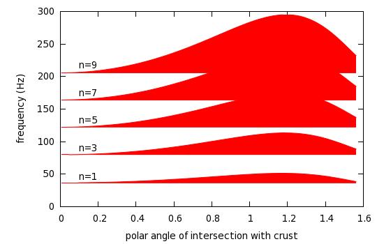
According to Sturm-Liouville theory the normalized eigenfunctions $\xi_{n}$ of Eq. (26) form an orthonormal basis with respect to the following inner product:

$\displaystyle\langle\xi_{m},\xi_{n}\rangle=\int_{0}^{\chi_{c}}r\left(\chi\right)\xi_{m}\left(\chi\right)\xi_{n}\left(\chi\right)d\chi=\delta_{m,n}$

(28)

Where $\delta_{m,n}$ is the Kronecker delta and $r=4\pi\rho/B_{\chi}$ is the weight function. We have checked that the solutions we find satisfy the orthogonality relations.

We are now ready to compute the coupled crust-core motion. Here we follow L07 and assume that the crust is an infinitely thin elastic shell⁶⁶ 6 It is straightforward to relax this assumption, and carry out the analysis of this section for the finite crustal thickness. However, from Section 2 it is clear that the interesting dynamics is dominated by the spectral structure of the core Alfven waves; therefore in order to flesh out the physics we choose the simplified model of the crust.. We label the lattitudinal location by the flux surface $\psi$ intersecting the crust, and consider the crustal axisymmetric displacements $\bar{\xi}_{\phi}(\psi)$. In the MHD approximation, the magnetic stresses enforce a no-slip boundary condition at the crust-core interface, such that $\xi_{\phi}\left(\psi,\chi_{c}\right)=\bar{\xi}_{\phi}\left(\psi,\chi_{c}\right)$ instead of $\xi_{\phi}\left(\psi,\chi_{c}\right)=0$. It is useful to make the following substitution

$\displaystyle\zeta\left(\psi,\chi\right)\equiv\xi_{\phi}\left(\psi,\chi\right)-\bar{\xi}_{\phi}\left(\psi\right)w\left(\psi,\chi\right)$

(29)

where we choose the function $w\left(\psi,\chi\right)$ so that (a) it corresponds to the static displacement in the core and hence satisfies $F\left(w\left(\psi,\chi\right)\right)=0$, and (2) $w\left(\psi,\chi_{c}\right)=1$. Therefore the new quantity satisfies the boundary condition $\zeta\left(\psi,\chi_{c}\right)=0$ and can be expanded into the Alfven normal modes $\xi_{n}$ which satisfy the same boundary conditions.

We now proceed by substituting Eq. (29) into Eq. (26) thus obtaining a simple equation of motion for $\zeta$

$\displaystyle\frac{\partial^{2}\zeta\left(\psi,\chi\right)}{\partial t^{2}}-F\left(\zeta\left(\psi,\chi\right)\right)=-w\left(\psi,\chi\right)\frac{\partial^{2}\bar{\xi}_{\phi}\left(\psi\right)}{\partial t^{2}}$

(30)

From the definition of the operator $F$ it follows that for the odd modes

$\displaystyle w\left(\psi,\chi\right)=x\left(\psi,\chi\right)\int_{0}^{\chi}\frac{K\left(\psi\right)}{x^{2}\left(\psi,\chi^{\prime}\right)B_{\chi}\left(\psi,\chi^{\prime}\right)}d\chi^{\prime}.$

(31)

Here the constant $K\left(\psi\right)$ is chosen such that $w\left(\psi,\chi_{c}\right)=1$, in order that $\zeta=0$ on both boundaries. We expand $\zeta$ and $w$ into a series of $\xi_{n}$’s:

	$\displaystyle\zeta\left(\psi,\chi,t\right)=\sum_{n}a_{n}\left(\psi,t\right)\xi_{n}\left(\psi,\chi\right)$		(32)
	$\displaystyle w\left(\psi,\chi\right)=\sum_{n}b_{n}\left(\psi\right)\xi_{n}\left(\psi,\chi\right)$		(33)

Eq. (30) reduces to the following equations of motion for the eigenmode amplitudes $a_{n}$

$\displaystyle\frac{\partial^{2}a_{n}\left(\psi\right)}{\partial t^{2}}+\sigma_{n}^{2}\left(\psi\right)a_{n}\left(\psi\right)=-b_{n}\left(\psi\right)\frac{\partial^{2}\bar{\xi}_{\phi}}{\partial t^{2}}$

(34)

These equations show how the core Alfven modes are driven by the motion of the crust. To close the system, we must address the motion of the crust driven by the hydromagnetic pull from the core.

The equation of motion for the crust is given by

$\displaystyle\frac{\partial^{2}\bar{\xi}_{\phi}}{\partial t^{2}}=L_{\rm el}\left(\bar{\xi}_{\phi}\right)+L_{B}$

(35)

Where the acceleration due to elastic stresses $L_{\rm el}$ is

$\displaystyle L_{\rm el}\left(\bar{\xi}_{\phi}\right)=\omega_{\rm el}^{2}\left[\frac{\partial^{2}\bar{\xi}_{\phi}}{\partial\theta^{2}}+\cot{\left(\theta\right)}\frac{\partial\bar{\xi}_{\phi}}{\partial\theta}-\left(\cot{\left(\theta\right)}^{2}-1\right)\bar{\xi}_{\phi}\right]$

(36)

where $\theta$ is the polar angle (cf. L07). The acceleration $L_{B}$ due to the magnetic stresses between the crust and the core can be expressed as

$\displaystyle L_{B}=-\frac{xB^{2}}{4\pi\Sigma}\cos{\alpha}\frac{\partial}{\partial\chi}\left(\frac{\xi_{\phi}}{x}\right)_{\chi=\chi_{\rm crust}}$

(37)

where $x$ is the distance to the axis of the star, $\Sigma$ is column mass-density of the crust and $\alpha$ is the angle between the magnetic field line and the normal vector of the crust.

It is convenient to express the crustal displacement $\bar{\xi}_{\phi}$ as a Fourier series, being a sum normal modes of the free-crust problem. Using Eq. (36) is straightforward to show analytically that the eigenfunctions $f_{l}$ of the free-crust problem (Eq. (35) with $L_{B}=0$) are

$\displaystyle f_{l}\left(\theta\right)\propto\frac{dY_{l0}\left(\theta\right)}{d\theta}$

(38)

with eigenfrequencies

$\displaystyle\omega_{l}=\omega_{\rm el}\sqrt{\left(l-1\right)\left(l+2\right)}$

(39)

Here $Y_{l0}$ is the $m=0$ spherical harmonic of degree $l$. The normalized functions $f_{l}$ form an orthonormal basis, so that

$\displaystyle\int_{0}^{\infty}f_{l}\left(\theta\right)f_{m}\left(\theta\right)\sin{\left(\theta\right)}d\theta=\delta_{l,m}$

(40)

where $\delta_{l,m}$ is again the Kronecker delta. The crustal displacement can then be expressed in terms of $f_{l}$

$\displaystyle\bar{\xi}_{\phi}\left(\theta,t\right)=\sum_{l}c_{l}\left(t\right)f_{l}\left(\theta\right)$

(41)

Substituting Eq. (41) into Eq. (35) we obtain the equations of motion for the crustal mode amplitudes $c_{l}$

$\displaystyle\frac{\partial^{2}c_{l}}{\partial t^{2}}+\omega_{l}^{2}c_{l}=\int_{0}^{\pi}L_{B}\left(\theta,t\right)f_{l}\left(\theta\right)\sin\theta d\theta$

(42)

We can express $L_{B}$ as

	$\displaystyle L_{B}\left(\psi,t\right)=-\frac{B_{\chi}^{2}\left(\psi\right)}{4\pi\Sigma}\cos{\left(\alpha\left(\psi\right)\right)}\left[\sum_{n}a_{n}\left(t\right)\frac{\partial\xi_{n}\left(\psi\right)}{\partial\chi}\right.$		(43)
	$\displaystyle\left.+\frac{K\left(\psi\right)}{x\left(\psi\right)B\left(\psi\right)}\sum_{k}c_{k}\left(t\right)f_{k}\left(\theta\left(\psi\right)\right)\right]_{\chi=\chi_{c}}$

Up to this point the derived equations of motion for the crust and the fluid core are exact. We are now ready to discretize the continuum by converting the integral of Eq. (42) into a sum over $N$ points $\theta_{i}$. In order to avoid the effect of phase coherence (see section 3) which caused drifts in the results from L07, we sample the continuum randomly over the $\theta$-interval $\left[0,\pi/2\right]$. In the following, functional dependence of the coordinate $\psi$ or $\theta\left(\psi\right)$ is substituted by the discrete index $i$ which denotes the $i$-th flux surface.

	$\displaystyle\frac{\partial^{2}c_{l}}{\partial t^{2}}+\omega_{l}^{2}c_{l}=2\sum_{i}L_{B}\left(\theta_{i},t\right)f_{il}\sin\theta_{i}\Delta\theta_{i}$		(44)
	$\displaystyle=-\sum_{i}\sin{\left(\theta_{i}\right)}\Delta\theta_{i}f_{il}\left[\frac{B_{\chi,i}^{2}}{2\pi\Sigma}\cos{\left(\alpha_{i}\right)}\left(\sum_{n}a_{in}\frac{\partial\xi_{in}}{\partial\chi}\right.\right.$
	$\displaystyle\left.\left.+\frac{K_{i}}{x_{i}B_{\chi,i}}\sum_{k}c_{k}f_{ik}\right)\right]_{\chi=\chi_{c}}$

$\displaystyle\frac{\partial^{2}a_{in}}{\partial t^{2}}+\sigma_{in}^{2}a_{in}=-b_{in}\sum_{l}\frac{\partial^{2}c_{l}}{\partial t^{2}}f_{il}$

(45)

These are the equations that fully describe dynamics of our magnetar model. As with the toy model from section 2 we integrate them using a second order leap-frog scheme which conserves the total energy to high precision. As a test we keep track of the total energy of the system during the simulations. Further we have checked our results by integrating equations (44) and (45) with the fourth-order Runge-Kutta scheme and found good agreement with leap-frog integration.

Based on our section-2 results, we have a good idea of what type of dynamical behavior should occur in our more realistic magnetar model. First, we expect that crustal modes with frequencies inside the Alfven continuum will be damped quickly by resonant absorption (”Landau-damping” in the terminology of Gruzinov 2008b). Second, as with our previous model we expect the late time behavior of the system to show QPO’s near the edges of the continuum, or edge modes. The third important feature of our model is that the continuum may possibly contain gaps, as is shown in Fig. 13. In this case there is the possibility that crustal frequencies fall inside the gaps and remain undamped. In all of our simulations these expectations have come true. We will now show the results from a simulation which illustrate the above mentioned effects.

The basic freedom of choice that we have for our model is the strength and geometry of the equilibrium magnetic field. We choose here a purely poloidal magnetic field with an average strength at the surface of $B_{\rm surf}=10^{15}~\rm G$, induced by a circular current loop of radius $a=0.5R_{*}$. This field gives us a gap in the continuum at frequencies $53<\omega<78~\rm Hz$.

We consider the lowest degree odd crustal modes with frequencies $\omega_{2}=40~\rm Hz$ and $\omega_{4}=84.5~\rm Hz$, which we couple to 5000 continuum oscillators (the Alfven continuum). We sample the continuum at 1000 randomly chosen flux surfaces, and at each flux surface we consider 5 Alfven overtones.

Like with our toy model from section 2, we initiate the simulation by displacing the crust ($c_{2}=c_{4}=1$) while keeping the continuum oscillators (the Alfven modes) relaxed ($a_{in}=0$).

In Figures 14 and 15 we show the resulting power spectrum for 2 different models. In the first one, the crustal frequencies are located inside the core continuum range, and the peaks due to the edge modes appear. By contrast, in the second case one of the crustal frequencies belongs to the gap, and a peak representing the global gap mode strongly stands our above the background. We note that the gap-mode’s frequency lies close to but does not coincide with the crustal-mode frequency; we found this to be a generic feature of our models, with the difference of $~10$% for the typical model parameters. The gap modes are particularly interesting because they have relatively large amplitudes, and are not as strongly damped by viscosity as the edge modes.

It must be emphasized that for all persistent modes in the system, the position in the frequency space of the core Alfven continuum plays the key role in setting the global-mode frequency and in determining its longevity.

We note that Lee (2008) has used a different method to identify discrete modes in a magnetar with similar magnetic configuration to ours. These modes were not associated with crustal frequencies, and we strongly suspect that they were located in the gaps of the continuum spectrum and could be identified with the edge or gap modes presented in this work.

To study this idea further, we specify a very simple model of a neutron star, motivated by the one considered in Levin (2006, hereafter L06) see Fig. 17 that never-the-less captures the essential physics.

Consider a perfectly conducting homogeneous fluid of density $\rho$ contained in a box with width $L_{x}$, length $L_{y}$ and depth $L_{z}$. The magnetic field in this box is everywhere aligned with the $y$-axis and its strength is a function of $x$ only. We assume that gravity is zero and consider a Lagrangian displacement $\xi\left(x,y,t\right)$ of the fluid along the $z$-direction; we specify periodic boundary conditions in this direction (one should think of the $z$ direction as azimuthal). We now add to this model a small effective shear modulus $\mu_{\rm eff}$ due to the field tangling. The fluid equation of motion is:

$$\frac{\partial^{2}\xi}{\partial t^{2}}=c_{A}^{2}\left(x\right)\frac{\partial^{2}\xi}{\partial y^{2}}+c_{s}^{2}\nabla^{2}\xi$$

(47)

Here $c_{A}\left(x\right)$ is the Alfven velocity and $c_{s}=\sqrt{\mu_{\rm eff}/\rho}$ is the $\mu_{\rm eff}$-generated shear velocity. If we assume a small shear speed, i.e. $c_{s}<<c_{A}$, Eq. (47) reduces to

$$\frac{\partial^{2}\xi}{\partial t^{2}}=c_{A}^{2}\left(x\right)\frac{\partial^{2}\xi}{\partial y^{2}}+c_{s}^{2}\frac{\partial^{2}\xi}{\partial x^{2}}.$$

(48)

We now find the core Alfven eigenmodes. After adapting the no-slip boundary conditions

	$\displaystyle\xi\left(-\frac{L_{x}}{2},y,t\right)=\xi\left(\frac{L_{x}}{2},y,t\right)=0,$
	$\displaystyle\xi\left(x,-\frac{L_{y}}{2},t\right)=\xi\left(x,\frac{L_{y}}{2},t\right)=0,$		(49)

the problem can be easily solved by separation of variables $\xi\left(x,y,t\right)\propto e^{i\omega t}\sin\left\{\pi m[(y/L_{y})+1/2]\right\}X\left(x\right)$, where $m=1,2,...$. Plugging this in Eq. (48) we find for the the $x-$dependent part of the solution:

$\displaystyle c_{s}^{2}\frac{\partial^{2}X}{\partial x^{2}}=\left[\omega^{2}-\omega_{A,m}^{2}\left(x\right)\right]X.$

(50)

Here $\omega_{A,m}\left(x\right)=\pi mc_{A}\left(x\right)/L_{y}$ can be interpreted as the frequency of the $m$-th Alfven overtone at $x$. From the above expression it is clear that in the limit of very small $c_{s}$, the solution for $X$ must be close to zero everywhere except in a very small neighborhood of $\omega_{A,m}(x)=\omega$. It is in this limit that the solutions are located on singular flux surfaces. However, in the presence of the non-vanishing shear velocity $c_{s}$, the eigenmodes spread out on neighboring field lines, effectively coupling the motion on different flux surfaces. The continuum of Alfven frequencies $\omega_{A,m}\left(x\right)$ will in this case be no longer solutions of the system. Instead, the coupling term gives rise to a discrete set of solutions rather than a continuum. Eq. (50) is the mathematical equivalent of Schrödingers equation, which can in general cases be solved numerically. However, for many special case exact solutions exist. Let us consider, for the sake of simplicity, a field configuration in our box such that:

$\displaystyle c_{A}^{2}\left(x\right)=a_{c_{A}}x^{2}+c_{A,0}^{2}$

(51)

We can rewrite Eq. (50) as follows:

$\displaystyle c_{s}^{2}\frac{\partial^{2}X}{\partial x^{2}}=-\frac{\pi^{2}m^{2}a_{c_{A}}}{L_{y}}x^{2}X+\left(\omega_{m}^{2}-\frac{\pi^{2}m^{2}c_{A,0}^{2}}{L_{y}}\right)X$

(52)

This differential equation is the mathematical equivalent of the quantum harmonic oscillator problem for which the exact solution is well known. The eigenfrequencies are given by

$\displaystyle\omega_{mn}^{2}=\pi\left(1+2n\right)mc_{s}\sqrt{a_{c_{A}}}/L_{y}+c_{A,0}^{2}\pi^{2}m^{2}/L_{y}.$

(53)

Here $n$ $(=0,1,...)$ is the ’quantum’ number labeling the harmonic-oscillator wavefunctions. We see that instead of a continuum, we obtain a densely packed discrete set of frequencies with the frequency spacing $\omega_{m,n}-\omega_{m,n-1}\sim\pi mc_{s}\sqrt{a_{c_{A}}}/L_{y}\omega_{m,n}$.

With the no-slip boundary conditions on the left and right sides $x=\pm L_{x}/2$, the eigenvalue equation must be solved numerically. An example of such calculation is shown in Fig. 18. There, the spacing between the discrete Alfven modes is shown to increase as one increases the effect of the field tangling characterized by the $\mu_{\rm eff}$.

We now introduce the crustal modes into the problem by making the top and bottom of the box elastic and mobile. We allow their displacement $\bar{\xi}_{t,b}(x,t)$ in the z-direction, and impose the boundary conditions on the sides:

$$\bar{\xi}_{t,b}(-L_{x}/2,t)=\bar{\xi}_{t,b}(L_{x}/2,t)=0.$$

(54)

Here the subscripts ”$t$” and ”$b$” stand for the top and bottom of the box, respectively. The top and bottom are assumed to be thin and have mass $M_{\rm cr}$ and surface density $\sigma=M_{\rm cr}/(L_{x}L_{z})$ . The crustal equation of motion is given by

	$\displaystyle{\partial^{2}\bar{\xi}_{t}\over\partial t^{2}}$	$\displaystyle=$	$\displaystyle v_{s}^{2}{\partial^{2}\bar{\xi}_{t}\over\partial x^{2}}-{\{B_{z}B_{x}\}_{t}\over 4\pi\sigma}$
	$\displaystyle{\partial^{2}\bar{\xi}_{b}\over\partial t^{2}}$	$\displaystyle=$	$\displaystyle v_{s}^{2}{\partial^{2}\bar{\xi}_{b}\over\partial x^{2}}+{\{B_{z}B_{x}\}_{b}\over 4\pi\sigma},$		(55)

where $v_{s}$ is the shear velocity in the crust. The crustal angular frequencies are given by $\omega^{\rm cr}_{j}=j\pi v_{s}/L_{y}$ with the corresponding crustal mode eigenfunctions $\bar{\xi}_{j}=\sin\{j\pi[(x/L_{x})+1/2]\}$ , where $j=1,2,...$ is roughly equivalent to $l$ in the spherical case. The symmetry of the problem allows one to consider either symmetric $\bar{\xi}_{t}=\bar{\xi}_{b}$ or antisymmetric $\bar{\xi}_{t}=-\bar{\xi}_{b}$ crustal modes. This will couple to the symmetric ($m=1,3,5,...$) or antisymmetric ($m=2,4,6,...$) Alfven modes of the core.

Just as in section 4, it is now convenient to define a new variable $\zeta(x,y,t)$ for the core displacement:

$$\zeta(x,y,t)=\xi(x,y,t)-\xi_{0}(x,y,t),$$

(56)

where

	$\displaystyle\xi_{0}(x,y,t)$	$\displaystyle=$	$\displaystyle{1\over 2}\left(\bar{\xi}_{t}(x,t)+\bar{\xi}_{b}(x,t)\right)$		(57)
		$\displaystyle+$	$\displaystyle\left(\bar{\xi}_{t}(x,t)-\bar{\xi}_{b}(x,t)\right){y\over L_{y}}.$

The new variable observes the regular boundary condition $\zeta=0$ on all the box edge, and satisfies the following inhomogeneous partial differential equation:

$$\left({\partial^{2}\over\partial t^{2}}-c_{A}^{2}(x){\partial^{2}\over\partial y^{2}}-c_{s}^{2}{\partial^{2}\over\partial x^{2}}\right)\zeta(x,y,t)=g(x,y,t),$$

(58)

where

$$g(x,y,t)=-\left({\partial^{2}\over\partial t^{2}}-c_{s}^{2}{\partial^{2}\over\partial x^{2}}\right)\xi_{0}(x,y,t).$$

(59)

The advantage of the new variable is that it satisfies the regular boundary condition $\zeta=0$ on all the boundaries of the box. It can therefore be expanded as a series consisting of eigenfunctions $\xi_{mn}$ of the right-hand side of Equation (48):

$$\zeta(x,y,t)=\Sigma_{mn}a_{mn}(t)\xi_{mn}(x,y).$$

(60)

The rest of the procedure is very similar to that in section 4. We expand the crustal displacement into a series consisting of the eigenmode wavefunctions $\bar{\xi}_{j}$:

	$\displaystyle\bar{\xi}_{t}(x,t)$	$\displaystyle=$	$\displaystyle\Sigma_{j}p_{j}(t)\bar{\xi}_{j}(x)$
	$\displaystyle\bar{\xi}_{b}(x,t)$	$\displaystyle=$	$\displaystyle\Sigma_{j}q_{j}(t)\bar{\xi}_{j}(x),$		(61)

where $p_{j}(t)$ and $q_{j}(t)$ are real numbers. The magnetar deformation is now fully represented by a set of generalized coordinates $[p_{j}(t),q_{j}(t),a_{mn}(t)]$. The coupled equations of motion are derived by following the procedure specified in section 4. We obtain the following system of equations:

	$\displaystyle\ddot{a}_{mn}+\omega_{mn}^{2}a_{mn}$	$\displaystyle=$	$\displaystyle-\Sigma_{j}\left[\ddot{p}_{j}+c_{s}^{2}\left({j\pi\over L_{x}}\right)^{2}p_{j}\right]\alpha^{(p)}_{(mn)j}$		(62)
			$\displaystyle-\Sigma_{j}\left[\ddot{q}_{j}+c_{s}^{2}\left({j\pi\over L_{x}}\right)^{2}q_{j}\right]\alpha^{(q)}_{(mn)j},$

and

	$\displaystyle\ddot{p}_{j}+{\omega^{\rm cr}_{j}}^{2}p_{j}$	$\displaystyle=$	$\displaystyle-{\rho c_{A}^{2}\over\sigma}\Sigma_{mn}\beta_{j(mn)}a_{mn}$		(63)
	$\displaystyle\ddot{q}_{j}+{\omega^{\rm cr}_{j}}^{2}q_{j}$	$\displaystyle=$	$\displaystyle-{\rho c_{A}^{2}\over\sigma}\Sigma_{mn}(-1)^{m+1}\beta_{j(mn)}a_{mn}$

where

	$\displaystyle\alpha^{(p)}_{(mn)j}$	$\displaystyle=$	$\displaystyle{\int\left({1\over 2}+{y\over L_{y}}\right)\xi_{mn}(x,y)\bar{\xi}_{j}(x)dxdy\over\int[\xi_{mn}(x,y)]^{2}dxdy}$
	$\displaystyle\alpha^{(q)}_{(mn)j}$	$\displaystyle=$	$\displaystyle{\int\left({1\over 2}-{y\over L_{y}}\right)\xi_{mn}(x,y)\bar{\xi}_{j}(x)dxdy\over\int[\xi_{mn}(x,y)]^{2}dxdy}$		(64)

and

$$\beta_{j(mn)}={\int\left({\partial\xi_{mn}(x,y)\over\partial y}\right)_{y=L_{y}/2}\bar{\xi}_{j}(x)dx\over\int[\bar{\xi}_{j}(x)]^{2}dx}.$$

(65)

Thus we have obtained a system of linear second-order differential equations, which describes the time evolution of the square-box magnetar. These equations are solved by trancating all the series [i.e., rescricting the range of indices $(m,n,j)$] and then by either solving the eigenvalue problem in order to find the normal modes, or by integrating the equations numerically⁸⁸ 8 Our favored method here is again the energy-conserving second-order leapfrog. It is both fast and stable over long integration times.. One then checks that the series trancation does not introduce errors in the magnetar’s motion within the frequency range of our interest.

References

Alpar, M. A., Langer, S. A., & Sauls, J. A. 1984, ApJ, 282, 533
Andersson, N., Glampedakis, K., & Samuelsson, L. 2009, MNRAS, 396, 894
Barat C. et al., 1983, A& A, 126, 400
Braithwaite, J. 2008, MNRAS, 386, 1947
Braithwaite, J., & Spruit, H. C. 2004, Nature, 431, 819
Braithwaite, J., & Nordlund, A. 2006, A&A, 450, 1077
Cerda-Duran, P., Stergioulas, N., & Font, J. 2009, MNRAS, 397, 1607
Colaiuda, A., Beyer, H., & Kokkotas, K.D. 2009, MNRAS, 396, 1441
Duncan, R. C. 1998, ApJ, 498, L45
Easson, I., & Pethick, C. J. 1979, 227, 995
Glampedakis K., Samuelsson L., & Andersson N., 2006, MNRAS, 371, L74
Goedbloed, J. P. H., & Poedts, S. 2004, Principles of Megnetohydrodynamics
(GP in the text; Cambridge University Press)
Gruzinov, A., 2008a, arXiv: 0801.4032 [astro-ph]
Gruzinov, A., 2008b, arXiv: 0812.1570 [astro-ph]
Gruzinov, A., 2009, arXiv: 0905.0911 [astro-ph]
Haensel P., & Potekhin A. Y., 2004, A&A, 428, 191
http://www.ioffe.ru/astro/NSG/NSEOS/
Haensel P., Potekhin A. Y., & Yakovlev D. G., 2007. Neutron Stars 1: Equation of State
and Structure (New York: Springer)
Hollweg, J. V. 1987, ApJ, 312, 880
Israel G. L. et al., 2005, ApJ, 628, L53
Ionson, J. A. 1978, ApJ, 226, 650
Landau, L. D., & Lifshits, E. M. 1976, Mechanics, chapter V
(Pergamon press)
Lee, U. 2008, MNRAS, 385, 2069
Levin Y., 2006, MNRAS Letters, 368, 35 (L06 in the text)
Levin Y., 2007, MNRAS, 377, 159 (L07 in the text)
Piro, A. 2005, ApJ, 634, L153
Poedts, S., Hermans, D., & Goossens, M. 1985, A&A, 151, 16 (P85 in the text)
Samuelsson, L., & Andersson, N. 2007, 374, 256
Sotani, H., Kokkotas, K. D., & Stergioulas, N. 2008, MNRAS Letters, 385, 5
Steiner W., & Watts A. L., 2009, Phys. Rev. Letters, 103r1101S
Strohmayer, T. E. & Watts, A. L., 2005, ApJ, 632, L111
van Hoven, M., & Levin, Y. 2008, MNRAS, 391, 283
Watts, A. L. & Strohmayer T. E., 2006, ApJ, 637, L117
Watts, A. L., & Reddy, S. 2007, MNRAS Letters, 379, 63
Appendix A Multimodal crust-core system
In this Appendix we generalize the normal-mode treatment of Section 2.2, and write down the general prescription of how to find the eigenmodes when several “large” crustal shear modes are coupled to a multitude of small core Alfven modes, provided the coupling coefficients are known. In this paper, the coupling coefficients are worked out in simple models of sections 4 and 5; we shall postpone the discussion of how the coefficients are computed in more general case to the future paper.
Let us denote the displacement of the crustal and core modes by and respectively. Since both the crustal and the core modes are not directly coupled to themselves (i.e., ’s are only coupled to ’s), most general equations of motion take the form