Multibreather and vortex breather stability in Klein–Gordon lattices: Equivalence between two different approaches
Abstract
In this work, we revisit the question of stability of multibreather configurations, i.e., discrete breathers with multiple excited sites at the anti-continuum limit of uncoupled oscillators. We present two methods that yield quantitative predictions about the Floquet multipliers of the linear stability analysis around such exponentially localized in space, time-periodic orbits, based on the Aubry band method and the MacKay effective Hamiltonian method and prove that their conclusions are equivalent. Subsequently, we showcase the usefulness of the methods by a series of case examples including one-dimensional multi-breathers, and two-dimensional vortex breathers in the case of a lattice of linearly coupled oscillators with the Morse potential and in that of the discrete model.
1 Introduction
Over the past two decades, there has been an explosion of interest towards the study of Intrinsic Localized Modes (ILMs), otherwise termed discrete breathers [1]. This activity has been, to a considerable extent, fueled by the ever-expanding applicability of these exponentially localized in space and periodic in time modes. A partial list of the relevant applications includes their emergence in halide-bridged transition metal complexes as e.g. in [2], their potential role in the formation of denaturation bubbles in the DNA double strand dynamics summarized e.g. in [3], their observation in driven micromechanical cantilever arrays as shown in [4], their investigation in coupled torsion pendula [5], electrical transmission lines [6], layered antiferromagnetic samples such as those of a (C2H5NH3)2CuCl4 [7], as well in nonlinear optics [8] and possibly in atomic physics of Bose-Einstein condensates [9, 10] and most recently even in granular crystals [11].
In parallel to the above experimental developments in this diverse set of areas, there has been a considerable progress towards the theoretical understanding of the existence and stability properties of such localized modes summarized in a number of reviews and books; see e.g. [1, 8, 12, 13]. Arguably, one of the most important developments in establishing the fundamental relevance of this area in coupled nonlinear oscillator chains has been the work of MacKay and Aubry [14], which established the fact that if a single oscillator has a periodic orbit (and relevant non-resonance conditions are satisfied), then upon inclusion of a non-vanishing coupling between adjacent such oscillators, an ILM type waveform will generically persist.
Given the confirmation of persistence of such modes, naturally, the next question concerns their robustness under the dynamical evolution of the relevant systems, which is critical towards their experimental observability. This proved to be a substantially more difficult question to answer in a quantitative fashion, especially so for ILMs featuring multiple localized peaks, i.e., multi-site breathers (since single-site breathers are typically stable in chains of linearly coupled anharmonic oscillators). Two principal theories were proposed for addressing the stability of such periodic orbit, discrete breather states (and identifying their corresponding Floquet multipliers). Interestingly, these originated independently from the same pioneers which established (jointly) the existence of such modes in [14]. In particular, the first theory was pioneered by Aubry in his seminal work of [12] and will go under the name Aubry Band (AB) theory, hereafter. The second one is an effective Hamiltonian method which was introduced in a series of papers by MacKay and collaborators [15] (and will be termed accordingly MacKay Effective Hamiltonian method (MEH)). The AB approach was adapted to the stability of discrete breathers and multibreathers in the setting of Klein-Gordon lattices in the work of [17]; see also [18]. The MEH approach was applied to the same setting in the recent work of [19]; see also [20].
Our aim in the present work is to unify the two methods by firmly establishing the equivalence of the stability conclusions of the Aubry band and MacKay effective Hamiltonian methods. Subsequently, we illustrate the usefulness and versatility of the methods, we apply them to a range of physically interesting chains of oscillator model examples, such as the Morse potential which arises in the study of DNA bubbles [3], as well as the potential which arises in applications in dusty plasmas [21], as well as in field theory, particle physics and elsewhere; see e.g. the recent discussion of [22] and the earlier review [23] and references therein. Our presentation is structured as follows. In section 2, we compare the two approaches and showcase the equivalence of their conclusions. In section 3, we study multibreathers and vortices in the case of the Morse potential. In section 4, we present the corresponding results for the Klein-Gordon lattice. Finally, in section 5, we summarize our findings and present our conclusions.
2 Comparison between the two approaches
2.1 Preliminaries - Terminology
The relevant system under consideration will be a Klein-Gordon chain of oscillators with nearest-neighbor interaction and Hamiltonian
| (1) |
As indicated previously, we will examine the two approaches (AB and MEH) for the linear stability of multi-site breathers of this general class of systems. Both approaches are based on the notion of the anti-continuum limit. In this limit () we consider “central” oscillators moving in periodic orbits with the same frequency (this will be our “multibreather” for ), while the rest lie at the equilibrium . For some of these configurations, depending on the phase differences between the oscillators, are continued in order to provide multibreather solutions. It is interesting/relevant to note here that while the MEH approach provides explicit conditions about which configurations can be continued to finite (the critical points of the relevant effective Hamiltonian), the AB theory provides only stability information for a given configuration (for which we already know otherwise that it should exist at finite ).
The linear stability of these solutions is determined by the corresponding Floquet multipliers. For a stable multibreather we require that all the multipliers lie on the unit circle. In the anti-continuum limit these multipliers lie in three bundles. The two conjugate ones, that correspond to the non-central oscillators, lie at , while the third one lie at and consists of multiplier pairs, corresponding to the central oscillators. Each pair of ’s correspond to the phase mode and growth mode of each isolated excited oscillator, meaning that a small change in the initial phase or a small change in frequency leads to an extremely close periodic solution, for the growth mode with slightly larger or smaller amplitude.
For , the non-central corresponding bundles split and their multipliers move along the unit circle to form the phonon band, while the multipliers at unity can move along, either the unit circle (stability), or along the real axis (instability). However, a pair of multipliers always continues at corresponding to the phase mode and growth mode of the whole system. Hence, the stability of the multibreather, at least for small values of the coupling, is determined by the multipliers of the central oscillators. For larger values of , a Hamiltonian-Hopf bifurcation can occur and destabilize an initially stable multibreather.
At this point, it is relevant to make a note in passing about the striking similarities between the discussion above (at and near the anti-continuum limit) with that of the linear stability of standing waves in the discrete nonlinear Schrödinger (DNLS) equation. In that case, due to the monochromatic nature of the solutions and the U invariance of the latter model, it is possible to directly consider the eigenvalues associated with the standing wave solutions. However, there is a direct analogy with the spectrum of the excited sites being associated with the eigenvalues at the origin at the anti-continuum limit and the continuous spectrum lying at a finite distance from the spectral plane origin, and how at finite coupling these zero eigenvalue pairs of the excited oscillators are the ones that may give rise to instability. In fact, it turns out that even the conditions under which instability will ensue for multibreathers of the KG directly parallel the ones for multi-breathers (or multi-site standing waves) of the DNLS. The latter are analyzed in considerable detail for , and dimensional settings in [13].
Returning to our KG setting, the MEH approach considers the Floquet multipliers given as , with , whereas in the AB approach, . Then,
| (2) |
Due to the symplectic character of the Floquet matrix if is a multiplier, so is , and due to its real character if a is non real multiplier, so is , where the asterisk denotes the complex conjugate. Therefore, the corresponding multipliers come in complex quadruplets if and is not real, or in duplets if is real, or if and not real. In addition, due to the time translation invariance of the system there is always a pair of eigenvalues at . This has as a result that both ’s and ’s, come also in quadruplets or duplets if is real, ( if is imaginary) or if is imaginary ( if is real). In principle, the duplets could collapse at a single value , but there is always a pair of ’s for the systems under study, as explained above.
2.2 The MEH approach
The MEH approach consists of constructing an effective Hamiltonian, whose critical points are in correspondence with periodic orbits (in our case multibreathers) of the original system. This method has been originally proposed in [15] and used in the present form in [16]. The effective Hamiltonian can be constructed as follows.
After considering the central oscillators we apply the action-angle canonical transformation to them. Note that, in the anticontinuous limit, the motion of the central oscillators, in the action-angle variables, is described by , for . Where is the angle, is the initial phase and the action of the -th central oscillator. For this kind of systems, the action of an oscillator can be calculated as
| (3) |
Since we are interested in a first order approach, the effective Hamiltonian can be written as , by neglecting terms which do not contribute to the results in this order of approximation. In this formula, is the average value of the coupling term of the Hamiltonian, over an angle in the anticontinuous limit, which is equivalent to the average value of over a period
This averaging procedure is performed in order to lift the phase degeneracy of the system. For the same reason we introduce a second canonical transformation
| (4) |
In these variables, the effective Hamiltonian reads
| (5) |
Note that, since the calculations are performed in the anticontinuous limit, the contribution of the non-central oscillators has disappeared.
As we seldom know the explicit form of the transformation , we use the fact that since the motion of the central oscillators for is periodic, and possesses the symmetry, it can be described by a cosine Fourier series
Note that at the anti-continuous limit, the orbits differ only in phase (i.e. ), therefore and the coefficients ’s do not depend on the index .
So, excluding the constant terms, becomes for the KG problem [19]
| (6) |
One of the main features of the MEH approach is that the critical points of this effective Hamiltonian correspond to the multibreather solutions of the system. This fact provides the corresponding persistence conditions, as the simple roots of . Remarkably, in this setting, similarly to what is known also for the DNLS [13], it can be proved that the only available multibreather solutions in the one-dimensional case are the ones with relative phase among the excited sites of or .
The second important fact the MEH approach yields is that the linear stability of these critical points (i.e., the Hessian of the effective Hamiltonian) determines the stability of the corresponding multibreather. In particular, the nonzero characteristic exponents of the central oscillators (see the discussion in the previous subsection) are given as eigenvalues of the stability matrix where is the matrix of the symplectic structure. By using the form in (5) for the we get:
Since the only permitted values of the relative phases are , or , the matrix simplifies considerably acquiring the form:
which, subsequently, if we consider only the dominant eigenvalue contributions, we get that , where are the eigenvalues of the matrix which reads
In this expression denotes the frequency, while
| (26) |
This leads to the characteristic exponents (i.e., effective eigenvalues) of the DB in the form:
| (27) |
with being the eigenvalues of the matrix
| (28) |
2.3 The AB approach
We demonstrate hereby that (27) can be reobtained based on the AB approach, by using the exposition of [17]. To this end, we recall that the aim of the AB approach is to look for the displacement that Aubry’s bands [12] experience when the coupling is switched on. What we plan to do below is to calculate the Floquet eigenvalues assuming that the bands are parabolic and their shape does not change when the coupling is introduced.
First, we recall the basics of Aubry’s band theory with the notation used in [17] adapted to the notation in the present paper, where convenient, for ease of comparison. The Hamilton equations applied to the Hamiltonian of Eq. (1) can be written as:
| (29) |
for a generic coupling potential , or, if it is harmonic:
| (30) |
where is a coupling constant matrix. Let us define († meaning the transpose matrix). Defining , and so on, Eq. (29) can be written as:
| (31) |
Suppose that is a time–periodic solution, with period and frequency , its (linear) stability depends on the characteristic equation for the Newton operator given by
| (32) |
where product is the list product, i.e., is the column matrix with elements , and is the matrix of functions , which depends on through .
If , this equation describes the evolution of small perturbations of , which determines the stability or instability of . It is however, extremely useful to consider the characteristic equation for any eigenvalue as it is the cornerstone for Aubry’s band theory.
Any solution of Eq. (32) is determined by the column matrix of the initial conditions for positions and momenta , with . A basis of solutions is given by the functions with initial conditions , , with .
The Newton operator depends on the –periodic solution , and therefore, it is also -periodic and its eigenfunctions can be chosen also as eigenfunctions of the operator of translation in time (a period ). They are the Bloch functions , being a column matrix of –periodic functions. The sets are also the eigenvectors of the Floquet operator or monodromy, that maps into , that is, . Their corresponding eigenvalues are the multipliers , with being the Floquet arguments.
The set of points , with being a real Floquet argument of , has a band structure. As the Newton and Floquet operators are real, the Floquet multipliers come in complex conjugate pairs. Therefore, if belongs to a band (i.e. is real), does it too, i.e., the bands are symmetric with respect to , which implies that . There are always two -periodic solutions, with Floquet multiplier () for . One is , which represents a change in phase of the solution and it is called the phase mode; the other is called the growth mode, given by , and represents a change in frequency and consequently in amplitude. The consequence is that there is always a symmetric band tangent to the axis at .
There are at most points for a given value of and, therefore, there are at most bands crossing the horizontal axes in the space of coordinates . The condition for linear stability of is equivalent to the existence of bands crossing the axis (including tangent points with their multiplicity). If a parameter like the coupling changes, the bands evolve continuously, and they can lose crossing points with , leading to an instability of the system.
The first item to find out are the bands at the anticontinuous limit, where Eq. (30) reduces to identical equations:
| (33) |
If we consider solutions around a minimum of , the oscillators can be at rest , or oscillating with period ; the latter are identical except for a change in the initial phase, so they can be written as with being the only -periodic, time-symmetric solution of Eq. (33) with . Therefore, the excited oscillators can be written as:
| (34) |
with if , and .
Let be the number of excited oscillators at the anticontinuous limit, labeled . Then, there are identical bands tangent to the axis at for each excited oscillator, and bands, corresponding to the oscillators at rest, with points intersecting the axis.
Thus, the excited bands can be approximated around by
| (35) |
with and being the eigenvalues of the -matrix defined below. Additionally,
| (36) |
where we have made use of [17, Eq. (B14)]. The factor is positive if the on-site potential is hard and negative if is soft (a potential is hard if the oscillation amplitude increases with the frequency and soft otherwise). When the coupling is switched on, the bands will move and change shape; the eigenvalue is degenerate with multiplicity at , but this degeneracy is generically lifted for and only one band will continue being tangent at due to the phase mode. Applying degenerate perturbation theory to Eq. (32), with being the perturbation, a perturbation matrix can be constructed [17], whose eigenvalues are those of the perturbed Newton operator. The non-diagonal elements of are given by
| (37) |
with . The diagonal elements are
| (38) |
If the on-site potential is homogeneous and the coupling is given as in Eq. (1), as is the case in the present paper, . Let us calculate the derivatives of , . Because of the way the diagonal elements of are constructed, we only need the derivatives with . It is easy to see that they are zero except for (defined below) for . The derivatives and are also zero as the oscillators at the extremes of the multibreather are not coupled between them. Then, the matrix becomes:
| (39) |
or, explicitly:
with
| (46) |
Then, by using [26, Lemma 5.4] we see that the matrices and have the same nonzero eigenvalues i.e.
| (47) |
In addition, has also a zero eigenvalue.
Some important values of are the following ones:
| (48) | |||||
| (49) |
For a Morse potential, ; for an even potential, .
According to the AB theory [12], the Floquet multipliers are given by the cuts of the bands with the axis; thus
| (50) |
and, applying the last results
| (51) |
where we have taken into account that 11 1 The expression comes from the Hamilton’s equations for the action-angle variables, since all the calculations are performed in the uncoupled, and therefore integrable, limit.
| (52) |
3 The Case Example of the Morse potential
3.1 Characteristic exponents
We now consider some special case examples, starting with a linearly coupled lattice of oscillators subject to the Morse potential. As indicated previously, the only configurations that may exist in the one-dimensional setting are ones which involve excited oscillators either in-phase (i.e., with ) or out-of-phase (i.e., with ); see [18], [19] and also [24] for a detailed discussion. Here, we proceed to perform some explicit calculations for the Floquet multipliers in the case of n-site breathers. In what follows we consider only the positive . To this end we express (27) making use of (47):22 2 In what follows, and in order to fix ideas, given the equivalence of the two methods, we will use the formulation with the -matrix.
| (53) |
where denotes the Q-matrix eigenvalues for a given . It is straightforward to show that33 3 We are neglecting the 0 eigenvalue, associated with .
| (54) |
and that
| (55) |
For instance, in the case of a 2-site breather, and .
We now focus on the particular case of the Morse potential, since it is a potential for which closed form analytical expressions can be found. [For other types of potentials, some approximations can be made for small and high frequencies; alternatively, the required single-oscillator parameters, such as and can be calculated numerically].
In the Morse case and in order to evaluate and , we express as a function of the Fourier coefficients:
| (56) |
For this potential,
| (57) |
Substituting into the action
| (58) |
Thus,
| (59) |
In the case of a general phase, we can express with given by (46). In the special case of the Morse potential, we have
| (60) |
To obtain the relevant sum, we use a simple geometric series formula that can be found e.g. in [25], according to which:
| (61) |
Consequently,
| (62) |
For the relevant values of for time-reversible multibreathers, we get:
| (63) |
| (64) |
Figures 1 and 2 show, respectively, the analytical eigenvalue predictions (dashed lines) for stable and unstable two-site and three-site breathers with the Morse potential and how they favorably compare to the corresponding numerical results (solid lines), obtained via a fully numerical linear stability analysis (and corresponding computation of the Floquet multipliers). It is clear that the predictions are very accurate close to the anti-continuum limit, and their validity becomes progressively limited for larger values of the coupling parameter , yet they yield a powerful qualitative and even quantitative (in the appropriate parametric regime) tool for tracking the stability of these localized modes. The figures also illustrate typical profiles of the corresponding two- and three-site ILMs.
 |
 |
 |
 |
 |
 |
 |
 |
3.2 Vortices in square lattices
The methodology can also be extended to lattices of higher dimensionality. We consider below some basic properties of discrete vortex breathers of different integer topological charges, in a square 2D lattice. Firstly, we consider square vortices over a single “plaquette” of the 2D lattice with , i.e., at the anti-continuum limit, the excited sites are , , and with a phase difference between nearest neighbors. This implies a perturbation matrix given by:
| (65) |
with given from (61) which is evaluated as:
| (66) |
This, in turn, upon use of Eq. (53) implies that
| (67) |
where are the eigenvalues of the matrix. This corresponds to the matrix of the normal modes of a 1D chain of 4 linearly coupled oscillators with periodic boundary conditions. Let us recall that for a system of coupled oscillators, the eigenvalues are given by:
| (68) |
in addition to the eigenvalue. In the present case of 4 oscillators with periodic boundary conditions, the nonzero eigenvalues are given by and , with the former being doubly degenerate. Thus, we have for vortices the following spectrum:
| (69) |
which implies stability for .
This type of analysis can be generalized for arbitrary values of the vorticity , leading to the conclusion that is the matrix of coupled oscillators, which implies that vortices with any integer topological charge will be stable for in the case of a lattice with an on-site Morse potential. For instance, in the case of the vortex, we obtain the explicit expressions for the eigenvalues:
| (70) |
It is important to highlight here some interesting differences between the above results and the case of the DNLS (and more generally that of even potentials in KG chains, including the case of the hard lattice considered below). In the latter class of problems, the vanishing of the odd coefficients in the Fourier expansion of the periodic orbit leads to the conclusion that and hence there is no contribution to the eigenvalues to leading order. This is the situation which has been characterized as “super-symmetric” in [13] and one in which the higher order contributions would be critical in determining the stability. Nevertheless, in the case considered herein, the asymmetry of the Morse potential produces a nonvanishing of and offers a corresponding nonzero leading order correction to the eigenvalues at O.
Figure 3 shows the dependence of stability eigenvalues for the and vortices and their comparison with the obtained fully numerical linear stability results as a function of the coupling . As can be observed in the figures, the approximation is less accurate in this case, although it is qualitatively correct. The reason for the partial disparity is that higher order contributions to the relevant eigenvalues (whose calculation is considerably more technically involved) lead to the observed splitting of all the doubly degenerate eigenvalue pairs. In the relevant cases, the analytical (dashed line) predictions can be seen to straddle the two observed numerical pairs.
 |
 |
4 The Case Example of the Hard Potential
The time evolution of a single oscillator in the hard potential, is given by:
| (71) |
where is a Jacobi elliptic function of modulus and is the complete elliptic integral of the first kind defined as .
The breather frequency is related to the modulus through:
| (72) |
The elliptic function can be expanded into a Fourier series leading to [28]:
| (73) |
where is the elliptic Nome which is defined as
| (74) |
In order to get and , we cannot use (26) and (46) because it is not possible to find a closed form expression. Instead, we use the integral expression:
| (75) |
After some manipulations (where it is crucial to apply [27, identity 171]), we obtain:
| (76) | |||||
where is the complete elliptic integral of the second kind defined as , is the Jacobi zeta function and .
For the action , a similar manipulation leads to
| (77) |
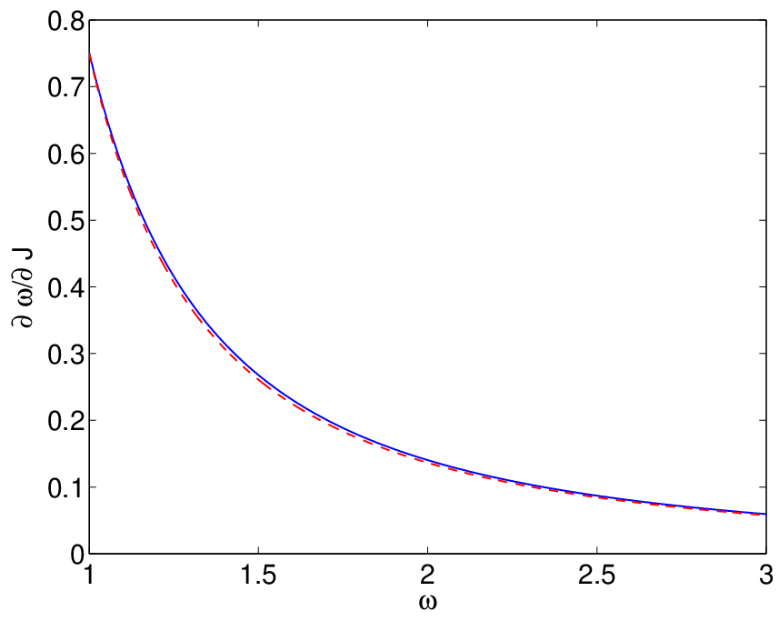
The derivative of this expression is cumbersome to handle. So, in what follows, we will work instead with numerically obtained values of and which are relevant for time-reversible multibreathers and vortex breathers, as for these cases we need , and . As indicated previously, for every even potential, , and, consequently, , and . This leads to:
| (78) |
| (79) |
Figure 4 shows the dependence of and with respect to the frequency. Figures 5 and 6 illustrate subsequently the relevant stability eigenvalues for 2-site and 3-site breathers as obtained from the expressions above and compare them to the full numerical linear stability results. The agreement in this case is very good (there are no degeneracies and associated higher-order contributions that may deteriorate the quality of the agreement as in the vortex breather case above); in fact, in some of the cases, the curves are almost indistinguishable throughout the considered parameter range.
An important observation concerns, however, the role of the “hard” nature of the potential. In particular, as illustrated in Fig. 4, the quantity is positive in this case, i.e., its sign is opposite from the soft case of the Morse potential (where ). This results in the corresponding reversal of the stability conclusions in Figs. 5 and 6, in comparison with Figs. 1 and 2 of the Morse case. That is, in-phase modes are now stable, while out-of-phase ones are unstable (as is true for the defocusing nonlinearity DNLS case also), while the reverse was true in the Morse potential (as well as for the focusing DNLS case). Lastly, we recall that since this is an even potential and thus , the leading order calculation would yield a vanishing contribution to the eigenvalues for the vortex case and a higher-order calculation is necessary to determine the stability of the latter.
 |
 |
 |
 |
 |
 |
 |
 |
 |
 |
As an aside towards obtaining a fully analytical prediction for this case (as some of the quantities need to be obtained numerically above), we note the following. Although we cannot acquire an exact form for , as in the case of the Morse potential, an approximate form for can be found by using the rotating wave approximation (RWA), i.e. by supposing that . The introduction in the dynamical equations for the single oscillator leads to:
| (80) |
Thus, and , and the corresponding expressions for the eigenvalues read:
| (81) |
| (82) |
A comparison between the numerically acquired values of and with the ones calculated from the RWA is shown in figure 4. The agreement is remarkable and attests to the quality of the “single frequency” rotating wave approximation. In Figs. 5 and 6 the characteristic exponents calculated numerically (solid lines) as well as using Eqs. (78)-(79) (dashed lines) and via Eqs. (81)-(82) are compared, illustrating the excellent agreement between all three.
5 Conclusions and Perspectives
The results presented in this work underscore the formulation of a toolbox that enables the systematic characterization of both the qualitative and even the quantitative aspects of stability of multibreather and vortex breather waveforms in these large number of degree of freedom, Hamiltonian lattice systems of the Klein-Gordon variety. A systematic calculation of the corresponding Floquet multipliers is presented and highlights the crucial components that imply stability, namely the proper combination of the sign of the coupling constant, the nature (hard or soft) of the potential and the relative phases between the adjacent excited sites. E.g., for positive couplings, and soft potentials, out-of-phase structures may be stable near the vanishing coupling limit, while in-phase ones are unstable; the nature of the conclusions is reversed for either (small) negative couplings or for hard potentials. The explicit analytical predictions have been tested against numerical results both for symmetric (such as the hard ) and asymmetric (such as the Morse) potentials, both for hard and soft ones, and both for simpler, non-degenerate one-dimensional multibreather settings and for more complex and degenerate two-dimensional vortex breathers. In all cases, the two theories whose results were shown to be equivalent herein, namely the Aubry band theory and the MacKay Effective Hamiltonian method yield excellent qualitative and good quantitative agreement with the full numerical linear stability results. The latter may not be true only in degenerate cases where higher order contributions may be critical in breaking the relevant degeneracy (as we saw in the case of the discrete vortices for the Morse model).
Naturally, a number of interesting directions for future consideration hereby arise. Perhaps the canonical one among them would involve a systematic derivation of higher order corrections for prototypical cases where the leading order approach yields vanishing results. For instance, the characterization of the stability of discrete vortices in the “super-symmetric” case of phase difference for even potentials would be a natural example. Another possibility that is also emerging and would be relevant to consider from a mathematical point of view would be to examine models with inter-site nonlinearities, such as ones of the Fermi-Pasta-Ulam type. In these cases, where the potential is a function , it is relevant to point out that upon consideration of the so-called strain variables , the problem is reverted to an on-site potential case, for which it would be worthwhile to explore methods similar to the ones analyzed herein. These directions are presently under consideration and will be reported in future publications.
Acknowledgments. PGK gratefully acknowledges support from NSF-DMS-0349023 (CAREER), NSF-DMS-0806762 and from the Alexander von Humboldt Foundation. JC and JFRA acknowledge financial support from the MICINN project FIS2008-04848.
References
- [1] S. Flach and C.R. Willis, Phys. Rep. 295, 182 (1998); S. Flach and A.V. Gorbach, Phys. Rep. 467, 1 (2008).
- [2] B.I. Swanson, J.A. Brozik, S.P. Love, G.F. Strouse, A.P. Shreve, A.R. Bishop, W.-Z. Wang, M.I. Salkola, Phys. Rev. Lett. 82, 3288 (1999).
- [3] M. Peyrard, Nonlinearity 17, R1 (2004).
- [4] M. Sato, B.E. Hubbard and A.J. Sievers, Rev. Mod. Phys. 78, 137 (2006).
- [5] J. Cuevas, L.Q. English, P.G. Kevrekidis and M. Anderson, Phys. Rev. Lett. 102, 224101 (2009).
- [6] L.Q. English, R. Basu-Thakur and R. Stearett, Phys. Rev. E 77, 066601 (2008).
- [7] L.Q. English, M. Sato and A.J. Sievers, J. Appl. Phys. 89, 6706 (2001); L.Q. English, M. Sato and A.J. Sievers, Phys. Rev. B 67, 024403 (2001).
- [8] F. Lederer, G.I. Stegeman, D.N. Christodoulides, G. Assanto, M. Segev and Y. Silberberg, Phys. Rep. 463, 1 (2008).
- [9] V.A. Brazhnyi and V.V. Konotop, Mod. Phys. Lett. B 18, 627 (2004).
- [10] O. Morsch and M.O. Oberthaler, Rev. Mod. Phys. 78, 179 (2006).
- [11] N. Boechler, G. Theocharis, S. Job, P.G. Kevrekidis, M.A. Porter, C. Daraio, arXiv:0911.2817.
- [12] S. Aubry. Physica D 103, 201 (1997).
- [13] P.G. Kevrekidis, The discrete nonlinear Schroödinger equation, Springer-Verlag (Berlin, 2009).
- [14] R.S. MacKay and S. Aubry, Nonlinearity 7, 1623 (1994).
- [15] T. Ahn, R.S. MacKay and J.-A. Sepulchre, Nonlinear Dyn. 25 157 (2001); R.S. MacKay and J.-A. Sepulchre, J. Phys. A 35 3985 (2002); R.S. MacKay, Energy Localisation and Transfer, T. Dauxois, A. Litvak-Hinenzon, R.S. MacKay, A. Spanoudaki (eds.), World Scientific, pp 149-192, (2004).
- [16] V. Koukouloyannis and R. S. MacKay, J. Phys. A: Math. Gen. 38, 1021 (2005).
- [17] J.F.R. Archilla, J. Cuevas, B. Sánchez-Rey, and A. Álvarez. Physica D 180, 235 (2003).
- [18] J. Cuevas, J.F.R. Archilla, and F.R. Romero. Nonlinearity 18, 76 (2005).
- [19] V. Koukouloyannis and P.G. Kevrekidis. Nonlinearity 22, 2269 (2009).
- [20] V. Koukouloyannis, P.G. Kevrekidis, K.J.H. Law, I. Kourakis, D.J. Frantzeskakis, J. Phys. A. Math. Theor. 43, 235101 (2010).
- [21] V. Koukouloyannis and I. Kourakis, Phys. Rev. E 76, 016402 (2007); V. Koukouloyannis and I. Kourakis, Phys. Rev. E 80, 026402 (2009).
- [22] D. Cubero, J. Cuevas and P.G. Kevrekidis, Phys. Rev. Lett. 102, 205505 (2009).
- [23] T.I. Belova, A.E. Kudryavtsev, Phys. Usp. 40, 359 (1997).
- [24] J. Cuevas. Localization and energy transfer in anharmonic inhomogeneus lattices. PhD Thesis, University of Sevilla (Spain), 2003.
- [25] I.S. Gradshteyn and I.M. Ryzhik. Table of integrals, series, and products. Academic Press (New York, 1965).
- [26] B. Sandstede. Trans. Am. Math. Soc., 350, 429 (1998).
- [27] A. Khare, A. Lakshminarayan, and U. Sukhatme. ArXiV:math-ph/0306028. This paper was published as Pramana 62 (2004) 1201, but the referred identity only appears in the preprint.
- [28] M. Abramowitz and I.A. Stegun. Handbook of mathematical functions. Dover (New York, 1965).