Planar Josephson Tunnel Junctions
in an Asymmetric Magnetic Field

in which the term $\mathcal{I}_{b}(X)$ is the distribution of the externally applied bias current $I_{b}$; choosing the $X$-axis origin in the center of the junction, $I_{b}=\int^{L/2}_{-L/2}\mathcal{I}_{b}(X)dX$. In normalized units of $x=X/\lambda_{j}$, Eq.(1) becomes:

With such normalization the junction length is $l=L/\lambda_{j}$; further, the Josephson (zero-voltage) current $i_{j}$ through the barrier is obtained as the spatial average of $\sin\phi$, $i_{j}=\left\langle\sin\phi\right\rangle=(1/l)\int_{-l/2}^{l/2}\sin\phi(x)dx$, while the total bias current $i_{b}=I_{b}/(J_{c}WL)$ is given by the spatial average of $\gamma$, $i_{b}=\left\langle\gamma\right\rangle$. In this work we will consider two quite different symmetric bias current profiles: i) uniform bias $\gamma(x)=\gamma_{u}$ for which $i_{b}=\gamma_{u}$ and ii) $\delta$-shaped bias $\gamma(x)=\gamma_{\delta}\delta(x)$ for which, being $\int_{-a}^{a}\delta(x)dx=1$, we have $i_{b}=\gamma_{\delta}/l$. $\delta$-biased JTJs in a uniform magnetic field have been the subject of a recent theoretical and experimental investigation[5, 6]. According to the magnetic Josephson equation[3], the boundary conditions for Eq.(2) depend on the external field values at the junction extremities:

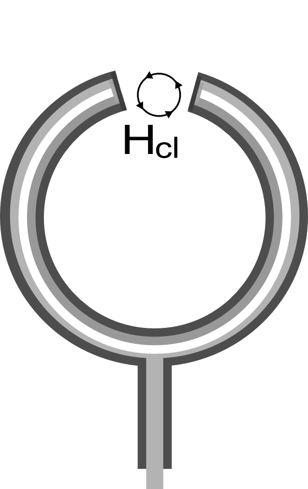
in which $h_{L,R}$ are the $Y$-components $H_{L,R}$ of the applied magnetic field at the left and right junction ends, normalized to $\Phi_{0}/(2\pi\mu_{0}d_{e}\lambda_{j})$. Classically one considers the case of a uniform field applied in the junction plane perpendicular to the long junction dimension $L$, so that $h_{R}=h_{L}$. We will refer to the above conditions as symmetric or classical boundary conditions to distinguish them from the asymmetric boundary conditions (ABC) achieved when the magnetic fields at the junction extremities have the same amplitudes, but opposite directions, that is, $h_{R}=-h_{L}\equiv h_{a}$. We will analyze the properties of ABC later on; for now we only remark that they reminds of the boundary conditions for an in-line symmetric junction[7] with $h_{L,R}$ being the self-fields produced by the external current which enters the junction at one extremity and leaves at the opposite one. Figs.1(a) and (b) show two examples of how the ABC could be realized in practical devices. In both cases the asymmetry is obtained by the current $I_{cl}$ flowing in a properly designed control line. The control line technique has been widely and successfully used to produce local magnetic fields in Josephson structures since 1994[8]. In Fig.1(a) the control line, separated from the junction by an insulating layer, runs aside the long dimension of an overlap-type planar JTJ and flips sides in the center of the junction. In the second, less easily achievable, case, sketched in Fig.1(b), the control line is perpendicular to the junction plane and goes through a small hole drilled in the substrate in between the gap of a ring shaped JTJ. In the former case the bias current density is uniform, while in the latter case the current distribution can be expressed in terms of a $\delta$-function[5]. It is quite evident that ABC are achieved in both electrode configurations.

The ABC have several important implications. We begin by computing the Josephson current $i_{j}$ carried by the junction. From Eq.(2) we easily get:

With the classical boundary conditions, the first term of the right side of Eq.(4) vanishes, so that $i_{j}=i_{b}$. However, with ABC we get:

i.e., the zero-voltage current also depends on the amplitude of the asymmetric magnetic field. More precisely, the applied magnetic field acts as an extra field-dependent d.c. current source $i_{h}=2h_{a}/l$ in parallel to the external current source $i_{b}$. In real units the normalized current $i_{h}$ corresponds to a supercurrent $I_{H}=i_{h}J_{c}WL=2H_{R}W$ proportional to the junction width $W$ (e.g., with $H_{R}=10$A/m and $W=3\mu$m, then $I_{H}=60\mu$A). Eq.(4) suggests that a planar JTJ can be used as a magnetic first order gradiometer based on the readout of the current $i_{h}$ supplied by a stand-alone (unbiased) JTJ. However, it should be realized that, since $i_{h}$ is a zero-voltage current, the internal impedance of the current source is null, so that no power can be delivered to an external resistive load.

From a mathematical point of view, the peculiarity of the ABC is that, provided that the current distribution is symmetric $\gamma(-x)=\gamma(x)$, the solutions of Eq.(2) have to be even functions, $\phi(x)=\phi(-x)$, meaning that the phase difference between the two junction extremities is always null: $\phi(l/2)-\phi(-l/2)=0$. As a consequence of the phase parity, we could limit our analysis to the spatial range $[0,l/2]$, with the condition in the origin to be found as follows. From Eq.(2), for any $0<x_{0}<l/2$, we can write:

Taking the limit $x_{0}\to 0$, the first integral vanishes, since $\phi(x)$ is a continuous function. If also the bias current density $\gamma(x)$ is continuous, then the second integral vanishes too, enforcing $\phi_{x}(0+)-\phi_{x}(0-)=0$. Being the phase derivative an odd function, $\phi_{x}(0+)+\phi_{x}(0-)=0$, it vanishes in the origin:

However, this is no longer true when the bias profile is discontinuous. In the case of a $\delta$-shaped bias, Eq.(6) leads to a discontinuity of the phase gradient in the origin[9, 5]: $\phi_{x}(0+)-\phi_{x}(0-)=\gamma_{\delta}$. Exploiting again the symmetry property of the phase gradient, we have: $\phi_{x}(0-)=\gamma_{\delta}/2$ and

To summarize, an overlap junction with ABC obeys Eq.(2) with the condition at $x=l/2$ as in Eq.(3):

and the condition in the origin given by Eq.(7) or (8) in the cases of continuous or $\delta$-shaped bias, respectively.

Since the phase profile of a junction with ABC has to be even, then, for small junctions ($l<1$), we can use the trial function $\phi(x)=ax^{2}+b|x|+\phi_{0}$, with the parameters $a$ and $b$ to be determined from the boundary conditions and $\phi_{0}$ treated as an integration constant. We will consider separately the cases of uniform bias and that of a $\delta$-shaped bias profile[10]. In the former case, in order to fulfill the condition in (7), then $b=0$ and, to satisfy (9), $a=h_{a}/l$, so that: $\phi(x)=h_{a}x^{2}/l+\phi_{0}$. The Josephson current $i_{j}$ can be computed from the above quadratic expression:

in which we have introduced Fresnel’s integrals defined by: $\int_{0}^{\bar{x}}\sin ax^{2}dx=\sqrt{{\pi}/{2a}}\,S\left(\sqrt{{2a}/{\pi}}\,{\bar{x}}\right)$ and $\int_{0}^{\bar{x}}\cos ax^{2}dx=\sqrt{{\pi}/{2a}}\,C\left(\sqrt{{2a}/{\pi}}\,{\bar{x}}\right)$ ($a>0$). The critical current $i_{c}$ can be found by maximizing (10) with respect to $\phi_{0}$. Introducing the quantity $h_{e}=\sqrt{|h_{a}|l/2\pi}$, we get a Fresnel (or near-field) magnetic diffraction pattern:

with $\phi_{0}(h_{e})=\tan^{-1}C(h_{e})/S(h_{e})$. In the limit $h_{e}\to 0$, $S(h_{e})\approx 0$ and $C(h_{e})\approx h_{e}$ so that $i_{c}(0)=1$. In the opposite limit, i.e., for $h_{e}\to\infty$, $S(h_{e})\approx C(h_{e})\approx 1/2$, so that $i_{c}(h_{a})\approx\sqrt{\pi/h_{a}l}$. Fig.2 shows the dependence of the critical current $i_{c}$ on the product $h_{a}l$ (that is independent on $\lambda_{j}$).

In the case of $\delta$-shaped bias, then, in order to satisfy the conditions in (8) and (9), $b=-\gamma_{\delta}/2$ and $2a=(2h_{a}+\gamma_{\delta})/l=i_{j}$, so that: $\phi(x)=i_{j}x^{2}/2-\gamma_{\delta}|x|/2+\phi_{0}$. When the modulus of the ratio $li_{j}/\gamma_{\delta}$ is much smaller than unity, the quadratic term can be disregarded. $i_{j}=0$ means that $\gamma_{\delta}=-2h_{a}$, i.e., the solution is piecewise linear:

Eq.(12) works well either for small junctions ($l<1$) or near the pattern minima ($i_{j}\approx 0$) or for large field values ($h>>2$). The Josephson current corresponding to Eq.(12) can be computed:

The critical current $i_{c}(h_{a})$ can be found by maximizing (13) with respect to $\phi_{0}$, to give:

The integration constant is the sawtooth function:

In other words, for a small $\delta$-biased JTJ with ABC we expect a Fraunhofer-like magnetic diffraction pattern with a field-periodicity twice larger than that of a small uniformly biased JTJ in a uniform magnetic field $h^{u}$, for which $i_{c}(h^{u})=\sin(h^{u}l/2)/(h^{u}l/2)$.

Eq.(2) with ABC has been numerically integrated in order to find the magnetic diffraction patterns $i_{c}(h_{a})$ of JTJs having lengths larger that $\lambda_{j}$. The details of the numerical technique can be found in Ref.[5] together with the analogous results in the case of symmetric boundary conditions. Figs.3(a)-(d) show the numerically obtained $i_{c}(h_{a})$ for JTJs with ABC having normalized lengths $l=2,4,8$ and $16$, respectively: the full dots refer to the uniform bias, while the open dots correspond to the point injected current. Note the very good agreement between the theoretical dependence of Fig.2 and the result of the numerical simulations for $l=2$ shown by the dashed line of Fig.3(a).

The validity of Eq.(5) has been numerically checked both in the case of uniform bias and $\delta$-shaped bias. In the latter case, for $l=2$, the phase profile could be well approximated by $\phi(x)=h_{a}x^{2}/l+\phi_{0}$ for $|h_{a}|<1$ ($0<\phi_{0}<\pi/2$) and by Eq.(12) for $|h_{a}|>1$ [with $\phi_{0}$ given by Eq.(15)]. For $l\geq 4$ the linear approximation is good for $|h_{a}|>2-3$. Generally speaking, it is observed that the magnetic diffraction patterns become more and more asymmetric as the junction normalized length increases. Parenthetically, we note that what is measured in the experiments is the maximum bias current that by virtue of Eq.(4) can be quite different from the critical current. This might explain why the effects of a non-perfectly uniform magnetic field have never been reported in the literature so far.

An asymmetric magnetic field drastically modifies also the dynamics of a planar JTJ. It is easy to see that the Josephson phase parity does not allow the standing wave resonances leading to current singularities such as Fiske and flux flow steps observed in presence of a uniform external field[11]. In fact, the magnetic field with opposite directions at the junction ends forces a chain of fluxons entering on one side and a chain of antifluxons entering on the other side, with the total magnetic flux in the barrier being always null. Furthermore, a small amplitude asymmetric field provides an asymmetric tuning of the average speed of one (or more) soliton shuttling back and forth along the junction, opposite to the symmetric tuning typical of a uniform field[12].

In summary, it has been discussed how the magnetic properties of a planar Josephson tunnel junction change when the textbook assumption of a perfectly homogeneous magnetic field is reverted into a fully asymmetric one. In the most general case when the magnetic field has different amplitudes at the junction extremities, due to the system non-linear nature, the problem cannot be split in two subproblems with properly chosen symmetric and asymmetric boundary conditions, unless the conditions for linearizing the current-phase relationship occur[13]. The experimental verification of our findings has been planned.

The author thanks V.P. Koshelets, J. Mygind, and R.J. Rivers for useful and stimulating discussions.

References

- [2] A. Barone and G. Paternò, Physics and Applications of the Josephson Effect (Wiley, New York, 1982); K.K. Likharev, Dynamics of Josephson Junctions and Circuits (Gordon & Breach Science Publishers, New York, 1984).
- [3] B. D. Josephson, Rev. Mod. Phys. 36, 216 (1964).
- [4] M. Weihnacht, Phys. Status Solidi 32, K169 (1969).
- [5] R. Monaco, J. Mygind, V.P. Koshelets and P. Dmitriev, Phys. Rev. B 81, 054506 (2010); cond-mat arXiv 0912.1510
- [6] R. Monaco, J. Mygind, R.J. Rivers, and V.P. Koshelets, Phys. Rev. B 80, 180501(R) (2009).
- [7] C.S. Owen and D.J. Scalapino, Phys. Rev.164, 538 (1967).
- [8] Y.M. Zhang, D. Winkler, P.A. Nilssnon, and T. Claeson, Appl. Phys. Letts.64, 1153 (1994).
- [9] M. Yu. Kuprianov, K.K. Likharev, V.K. Semenov, Fiz. Nizk. Temp.2, 1252 (1967); Sov. J. Low Temp. Phys.2, 610 (1976).
- [10] When the junction normalized length is much smaller than unity, then any electrode configuration will result in an uniform bias.
- [11] I.O. Kulik and I. K. Yanson, The Josephson Effect in Superconductive Tunneling Structures (Izdatel’stvo ”Nauka”, Moskow, 1970. Israel Program for Scientific Translations, Jerusalem, 1972).
- [12] O.A. Levring, N.F. Pedersen and M.R. Samuelsen, J. Appl. Phys. 84, 987-991 (1983); M.P. Soerensen, R.D. Parmentier, P.L. Christiansen, O. Skovgaard, B. Dueholm, E. Joergensen, V.P. Koshelets, O.A. Levring, R. Monaco, J. Mygind, N.F. Pedersen, M.R. Samuelsen, Phys. Rev. B30, 2640-2648 (1984).
- [13] A. Barone, W.J. Johnson and R. Vaglio, J. Appl. Phys.46, 3628 (1975).