Balancing congestion for unsplittable routing on a bidirected ringThanks: France Telecom Research & Development / BIZZ / DIAM. e-mail: Alexandre.Laugier@francetelecom.com

In this paper a bidirected ring means the union of two oppositely directed circuits on the same set of nodes. The motivation of the present paper is to compute a routing of demands in an SDH (Synchronous Digital Hierarchy) based network. Such a network is a transmission network and we will refer to it as the supply graph. Also, we will refer to the set of demands as the demand graph. The backbone networks of the European telecommunication companies are based on the SDH technology. The ring architecture plays a key role in this technology, because it provides an efficient self-healing mechanism in case of failure: although the rings are bidirected, only one direction is used, while the other would be useful in case of a failure. Most of the SDH backbone networks consist of such uni-directed circuits. From such uni-directed circuits different topologies have been built, like tree of circuits or cycle of circuits. In the next section we will show that the routing in a supply graph which is a cycle of circuits can be reduced to a routing problem in a bidirected ring. One can find more about the SDH transmission protocol in [4].

Formally, we are given a directed supply graph $G$ with capacity function $c\colon E(G)\rightarrow\mathbb{R}_{+}$ and a directed demand graph $H$ on the same node set with demand values $d\colon E(H)\rightarrow\mathbb{R}_{+}$. A routing of $H$ is a collection of $uv$-paths of value $k$, one for each demand edge of $E(H)$ joining $u$ to $v$ with value $k$, satisfying the capacity constraint $c$. Since each demand is routed along a unique path we will speak about unsplittable routings. In this paper a routing is always unsplittable, unless when speaking about the fractional solution of the linear relaxation of the problem. We say that a routing of $H$ has load at most (less than) $c$ if for each edge $e\in E(G)$ the sum of the values of the paths using $e$ is at most (less than) $c(e)$.

In this paper we consider the routing problem in bidirected rings. Given a bidirected ring $G$ with capacity function $c\,\colon\,E(G)\rightarrow\mathbb{R}_{+}$, and a directed demand graph $H$ with demand values $d\colon E(H)\rightarrow\mathbb{R}_{+}$, we want to find the minimum $\alpha$ for which there exists a routing of $H$ with load at most $\alpha c$. This is called the balanced bidirected ring routing problem. Under balancedness we mean that the value of $\alpha$ is introduced to ensure that the remaining capacities are as large as possible, allowing the network to carry larger demands. The case when $c$ is uniform (that is, all capacities are equal) and each demand is 1 was solved with an elegant method by Wilfong and Winkler [5]. In Section 3 we follow the lines of their proof to give an algorithm which returns a routing with load less than $\alpha_{opt}c+\frac{3}{2}D$ where $\alpha_{opt}$ is the optimum solution of the problem and $D$ is the maximum value of the demands. We also show that this error term can indeed occur.

In Section 4, using a method of Khanna [2], we show an approximation scheme to the problem which for any $\varepsilon>0$ yields a routing with load less than $\alpha_{opt}(c+\varepsilon\frac{\sum c}{n})$, with a trade-off with the running time. Here $n=|V(G)|$ and $\sum c$ is the sum of the capacities of the edges.

By solving a linear program, a fractional solution of the balanced bidirected ring routing problem can be given, that is, we can calculate the minimum $\alpha$, denoted by $\alpha^{*}$, such that there exists a fractional routing of $H$ with load at most $\alpha c$. Clearly $\alpha^{*}\leq\alpha_{opt}$. Our approximation algorithm for the balanced bidirected ring routing problem gives a routing such that its load is actually less than $\alpha^{*}c+\frac{3}{2}D$. If $\alpha^{*}<1$ then our solution may be considered good in practice since it requires less than $\frac{3}{2}D$ additional capacity on each edge. On the other hand, if $\alpha^{*}\geq 1$ then there exists no feasible routing with the given capacities. Hence we are facing a network design problem, and our goal is to increase the capacity function with minimum cost, in order to have a routing satisfying the increased capacity. We show in Section 5 that even this problem can be handled with techniques similar to Section 3.

If the capacity function $c$ is uniform and the ring is undirected, the balanced ring routing problem was studied by many researchers due to its significance in telecommunication networks. This problem is called the undirected ring loading problem, first considered by Cosares and Saniee [1]. Schrijver, Seymour, and Winkler [3] gave a combinatorial approximation algorithm for the undirected case, if $c$ is not necessarily uniform. Their algorithm returns a routing requiring less than $\frac{3}{2}D$ more capacities on each edge than in an optimum solution. The balanced bidirected ring routing problem was first considered by Wilfong and Winkler [5] who gave an exact algorithm for finding an optimum routing in a bidirected ring, in case $c$ is uniform and each demand is 1. Our considerations in Section 3 are based on their method, yielding a generalization of their result. Our result are more general than theirs in the aspect that in our case the demands are not restricted to be 1, and the capacity function is not necessarily uniform.

We point out that the balanced bidirected ring routing problem is NP-complete. Indeed, the partition problem can be reduced to it in a straightforward way, just as in the undirected case (Cosares, Saniee [1]). Moreover, contrary to the undirected case, the cut condition is not sufficient for the existence of a fractional solution. That may be the reason that no combinatorial algorithm is known finding an optimum fractional solution of the bidirected ring routing problem, unlike in the undirected case.

In some SDH backbone networks the supply graph $G$ forms a cycle of directed circuits, with capacity function $c:E(G)\rightarrow\mathbb{R}_{+}$. In this section we show that the routing in $G$ can be reduced to a routing problem in a bidirected ring. Two neighboring circuits of $G$ meet in a node called a common node. The common nodes divide each directed circuit into two edge sets, called arcs. See Figure 1.

Let $f\in E(H)$ be a demand edge with value $d$ joining $v_{1}$ to $v_{2}$. Let $a_{1}$ be the common node $a$ of $G$ minimizing $dist_{G}(v_{1},a)$. Similarly, let $a_{2}$ be the common node $a$ minimizing $dist_{G}(a,v_{2})$. If $v_{2}$ is contained in the $v_{1}a_{1}$-path of $G$ then only one $v_{1}v_{2}$-path exists in $G$ so simply delete $f$ from $H$ and decrease the capacity of this path by $d$. Otherwise all $v_{1}v_{2}$-paths use the supply edges on the $v_{1}a_{1}$- and on the $a_{2}v_{2}$-paths of $G$. So replace $f$ by a new demand edge $f^{\prime}$ joining $a_{1}$ to $a_{2}$ with value $d$ and decrease the capacities of the supply edges on the $v_{1}a_{1}$ and on the $a_{2}v_{2}$-paths by $d$. After doing so for each demand edge, the new demand graph $H^{\prime}$ has a routing in $G$ with load at most the new capacity function $c^{\prime}$ if and only if $H$ has a routing with load at most $c$. Moreover, the non-common nodes of $G$ are incident to no edge of $H^{\prime}$, so we can think of an arc $A$ as only one edge with capacity the minimum of $c^{\prime}(e)$ taken over all edges $e\in A$. The new supply graph is a bidirected ring with $n$ nodes and $2n$ edges, where $n$ is the number of circuits in $G$.

In this section we show an algorithm yielding a routing in a bidirected ring with load less than $\alpha_{opt}c+\frac{3}{2}D$ where $\alpha_{opt}$ is the solution of the balanced bidirected ring routing problem and $D$ is the maximum value of the demands. Our algorithm is a modification of that of Wilfong and Winkler [5] who solved the balanced bidirected ring routing problem in the case if $c$ is uniform and the demands are $1$. We do not count running times since solving a linear program is included.

From the two directions of the ring we say that one is the forward and the other one is the backward direction. Accordingly, an edge $e\in E(G)$ can be forward or backward, and from the two possible $uv$-paths ($u,v\in V(G)$) one is the forward and the other one is the backward path. For an edge $f\in E(H)$ joining $u$ to $v$, an $f$-path refers to any of the two $uv$-paths of $G$. The edge sets of these two paths will be denoted by $F(f)$ and $B(f)$, respectively.

The first step is to solve the LP-relaxation of the problem. There are two possibilities of routing demand $f\in E(H)$ hence we introduce a variable $0\leq\varphi(f)\leq 1$ with the meaning that $\varphi(f)$ fraction of the demand $f$ is routed forward and $1-\varphi(f)$ fraction is routed backward. So we have the following LP-relaxation, whose optimum solution is denoted by $\alpha^{*}$. Both sums run on demand edges $f\in E(H)$.

Note that we would get $\alpha_{opt}$ if $\varphi$ was required to be integer. Now we manipulate the demands $f\in E(H)$ with $0<\varphi(f)<1$. Such demands are called split. We say that demands $f_{1},\,f_{2}\in E(H)$, where $f_{i}$ joins $s_{i}$ to $t_{i}$ for $i=1,2$, are parallel if the end nodes are placed in the ring in the order $s_{1},\,t_{1},\,t_{2},\,s_{2}$ (some of these nodes may coincide). Assume that $f_{1},\,f_{2}\in E(H)$ are parallel split demands. Call the $f_{i}$-path containing both $s_{3-i}$ and $t_{3-i}$ the long $f_{i}$-path for $i=1,2$. Let $x_{i}$ denote the amount of flow of $f_{i}$ sent along the long $f_{i}$-path in our fractional solution. If we reroute $\min(x_{1},x_{2})$ amount of flow from the long $f_{i}$-path to the other $f_{i}$-path for $i=1,2$ then one of the demands $f_{1},\,f_{2}$ will not be split any more, moreover, we do not increase the load of any edge of $G$ (we may even decrease it somewhere). So at most $|E(H)|$ such uncrossing steps are possible and finally we get a fractional solution where there are no pair of parallel split demands. Especially, demands with the same source node are parallel. So it will hold that for each $s\in V(G)$ there exists at most one split demand $f\in E(H)$ with source $s$.

Denote the nodes of $G$ by $s_{1},\,\ldots,\,s_{n}$ in the forward order. Now we try to unsplit the remaining split demands. Let $f_{i}$ be the split demand with source $s_{i}$ (if any). Assume that $x_{i}$ fraction of $f_{i}$ is routed forward and $y_{i}$ fraction backward. Let $w_{i}=y_{i}$ if we would set $\varphi(f_{i})$ to 1 and $w_{i}=-x_{i}$ if $\varphi(f_{i})$ would be set to 0. If we round $\varphi(f_{i})$ to 0 or 1 then the load of an edge $e\in E(G)$ increases by $w_{i}$ if $e$ is contained in the forward $f_{i}$-path, it decreases by $w_{i}$ if $e$ is contained in the backward $f_{i}$-path, and it does not change elsewhere. There are no two parallel split demands so the change of the load of an edge is $\pm\sum_{j\leq i\leq k}w_{i}$ for some $j\leq k$ where $k$ may be greater than $n$ but then the indices of $w$ are meant modulo $n$. Here the sign depends on whether $e$ is a forward or a backward edge. Now we try to set the value of $w_{i}$ to $y_{i}$ or $-x_{i}$ for all $i$ in such a way that $|\sum_{j\leq i\leq k}w_{i}|<\frac{3}{2}D$ holds for all $j\leq k$. To achieve this it is clearly sufficient that

(2) can be easily achieved by greedily setting the values $w_{i}$ to $y_{i}$ or $-x_{i}$ one after another, since $x_{i}+y_{i}\leq D$ holds. Hence by this procedure each load is increased by less than $\frac{3}{2}D$.

So the algorithm for the balanced bidirected ring routing problem is the following.

1. 1.

   Solve the LP-relaxation of the balanced bidirected ring routing problem.

2. 2.

   Uncross the parallel split demands.

3. 3.

   Unsplit the remaining split demands in the above described greedy way.

Our goal was to find a routing with load at most $\alpha_{opt}c+\frac{3}{2}D$, but actually, similarly to the undirected case [3], the routing we got has load less than $\alpha^{*}c+\frac{3}{2}D\leq\alpha_{opt}c+\frac{3}{2}D$. However, this fact does not always induce improved efficiency. Indeed, next we show that for every $\delta>0$ there is an example where the output routing of the algorithm has load not less than $\alpha_{opt}c+\frac{3}{2}D-\delta$. Such tight examples are very important in understanding how algorithms can be improved in order to decrease running time.

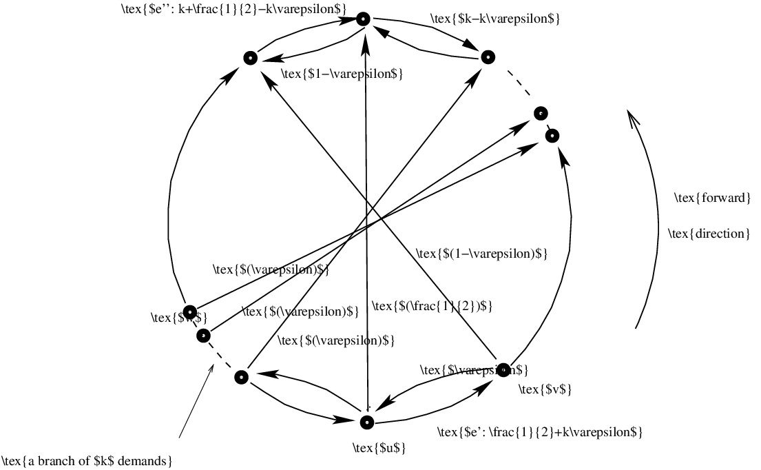
Consider the capacities of the ring as shown in Figure 2. The edges without capacity, as well as the dashed edges have large capacities in both directions and $\varepsilon$ is a number which is small enough with respect to $k$. All demands are of value $1$. Observe that the cut $\{e^{\prime},\,e^{\prime\prime}\}$ is tight, that is, the total value of the demands crossing it equals $c(e^{\prime})+c(e^{\prime\prime})$. It is easy to see that there is no integer routing with $\alpha=1$ due to the cut $\{e^{\prime},\,e^{\prime\prime}\}$ with fractional capacities. The best integer solution is obtained if the capacity of $e^{\prime\prime}$ is raised to $k+1$, that is $\alpha_{opt}^{(k)}=\frac{k+1}{k+\frac{1}{2}-k\varepsilon}$. Indeed, $\varepsilon$ is small enough so we can route the demand of node $v$ forward while all other demands backward. Thus $\lim_{k\to\infty}\alpha_{opt}^{(k)}=1$ by an appropriate choice of $\varepsilon=\varepsilon^{(k)}$.

Clearly $\alpha^{*}=1$, and an optimum $\varphi$ (which is a vertex of the polyhedron (1)) is shown in brackets in Figure 2. Assume that the unsplitting procedure starts at node $u$. The split demand at node $u$ is routed forward. Now the split demand at node $v$ is routed backward and then the demand of node $w$ forward. All remaining demands will be routed backward, according to our greedy heuristic. Now $e^{\prime}$ has load $2$ and so the error at $e^{\prime}$ tends to

by choosing $k\varepsilon\to 0$, and using that $D=1$. Note that the fractional capacities can be made integer by scaling.

If the value of the demands are small with respect to the minimum load of an optimum routing then the $\frac{3}{2}D$ additive error is a small deviation from the optimum solution. Otherwise this error term can be significant. In this section we develop an approximation scheme for the balanced bidirected ring routing problem, which for any $\varepsilon>0$ gives an algorithm polynomial in the number of nodes, finding a routing with load less than $\alpha_{opt}(c+\varepsilon\overline{c})$ where $n=|V(G)|$, and $\overline{c}=\frac{\sum_{e\in E(G)}c(e)}{n}$. We use the solution method of Khanna [2] who presented an $\varepsilon$-approximation scheme for the case of an undirected ring with $c$ uniform. By definition, an $\varepsilon$-approximation scheme for a minimization problem is an algorithm which, for any $\varepsilon>0$, returns a solution with value at most $1+\varepsilon$ times the optimum value. In this sense the method of this section is not an $\varepsilon$-approximation scheme since it does not approximate $\alpha_{opt}$. However, for $M>0$, in the class of balanced bidirected ring routing problem instances, where $\overline{c}\leq Mc(e)$ holds for all edge $e$, our method is an $M\varepsilon$-approximation scheme. Many problem instances in practice arising from an SDH backbone network belong to such a class with reasonably small $M$, in particular the instances where $c$ is uniform.

For $s,t\in V(G)$ the long $st$-path is defined to be the longest $st$-path in $G$, or to be the forward one if the two paths are of equal length. Recall that $\alpha^{*}$ denotes the fractional optimum to the balanced bidirected ring routing problem. Let $\alpha^{\prime}\geq\alpha^{*}$ be any real number and let

$E^{\prime}=\left\{f\in E(H)\,:\,d(f)>\frac{2}{3}\varepsilon\alpha^{\prime}\overline{c}\right\}.$

Note that

$\alpha^{\prime}\sum_{e\in E(G)}c(e)\geq\alpha^{*}\sum_{e\in E(G)}c(e)\geq\sum_{f\in E^{\prime}}d(f)>|E^{\prime}|\frac{2}{3}\varepsilon\alpha^{\prime}\overline{c}.$

Hence $|E^{\prime}|<\frac{3}{2\varepsilon}n$. If $\alpha^{\prime}\geq\alpha_{opt}$ then less than $\frac{3}{\varepsilon}$ edges of $E^{\prime}$ are routed in the long path in any optimum routing, since otherwise the sum of the loads would be more than

$\frac{2}{3}\varepsilon\alpha^{\prime}\overline{c}\cdot\frac{3}{\varepsilon}\cdot\frac{n}{2}=n\alpha^{\prime}\overline{c}=\alpha^{\prime}\sum_{e\in E(G)}c(e)\geq\alpha_{opt}\sum_{e\in E(G)}c(e),$

which is impossible. Thus, independently of whether $\alpha^{\prime}\geq\alpha_{opt}$ or not, for all subsets $E^{\prime\prime}\subseteq E^{\prime}$ with $|E^{\prime\prime}|<\frac{3}{\varepsilon}$ we do the following. We route the demands of $E^{\prime\prime}$ in the long paths and the demands of $E^{\prime}-E^{\prime\prime}$ in the short paths. Denote the load of $e\in E(G)$ in this routing of $E^{\prime}$ by $l(e)$. Now denote by $\alpha^{*}_{E^{\prime\prime}}$ the optimum of the following linear program, where the sums run on $f\in E(H)-E^{\prime}$.

Note that the maximum value of a demand in $E(H)-E^{\prime}$ is at most $\frac{2}{3}\varepsilon\alpha^{\prime}\overline{c}$. Hence exactly as in the previous section, we can find a routing of $E(H)-E^{\prime}$ with load less than $\alpha^{*}_{E^{\prime\prime}}c-l+\varepsilon\alpha^{\prime}\overline{c}$. In the case when $\alpha^{\prime}\geq\alpha_{opt}$, in any optimum routing of $H$ less than $\frac{3}{\varepsilon}$ edges of $E^{\prime}$ are routed in the long path, hence we get that one of the above routings has load less than $\alpha_{opt}c+\varepsilon\alpha^{\prime}\overline{c}$. For any $\alpha^{\prime}$, from these $\sum_{i=0}^{3/\varepsilon}\dbinom{|E^{\prime}|}{i}$ routings of $E(H)$ choose the one with load at most $\alpha c+\varepsilon\alpha^{\prime}\overline{c}$, such that this $\alpha$ is minimum.

The number of subsets $E^{\prime\prime}\subseteq E^{\prime}$ to consider is $\sum_{i=0}^{3/\varepsilon}\dbinom{|E^{\prime}|}{i}$. Using that $\dbinom{k}{l}\leq(ek)^{l}/l^{l}$ holds for any integers $k\geq l$, when $|E^{\prime}|\geq\frac{6}{\varepsilon}$ we get

Since the left hand side is monotone increasing in $|E^{\prime}|$, the above bound is valid when $|E^{\prime}|<\frac{6}{\varepsilon}$, too. Hence the number of subsets $E^{\prime\prime}\subseteq E^{\prime}$ to try is $O_{\varepsilon}(n^{\frac{3}{\varepsilon}})$.

Now we show how $\alpha^{\prime}$ can be chosen. It is clear that $\alpha^{*}\leq\alpha_{opt}\leq 2\alpha^{*}$, since there are exactly two paths between any two nodes in $G$. So first determine the value of $\alpha^{*}$ and then run the above algorithm with $\alpha^{\prime}=\alpha_{i}=\frac{N+i}{N}\alpha^{*}$ for $i=0,\ldots,N$ for some integer $N$. As we mentioned, at the point when $\alpha_{opt}\leq\alpha_{j}\leq(1+1/N)\alpha_{opt}$ happens to hold, our routing has load less than $\alpha_{opt}(c+\varepsilon(1+1/N)\overline{c})$. Thus, finally, from these $N+1$ routings choose the one with load at most $\alpha(c+\varepsilon(1+1/N)\overline{c})$, such that this $\alpha$ is minimum. In the beginning we should also replace $\varepsilon$ by $\varepsilon/(1+1/N)$ in the above scheme.

The approximation algorithm presented in Section 3 gives a routing in a bidirected ring with load less than $\alpha^{*}c+\frac{3}{2}D$. Recall that we can calculate the fractional optimum $\alpha^{*}$ by solving a linear program. Observe that $\alpha^{*}<1$ means that there exists a fractional routing in the supply network $G$ with the given capacities. Since our approximate integer solution requires less than $\frac{3}{2}D$ additional capacity on each edge (hopefully, much less on average), this solution may be considered good in practice. On the other hand, if $\alpha^{*}\geq 1$ then there exists no feasible routing with the given capacities. Hence we are facing a network design problem, where we want to increase the capacity of some edges of the ring, with minimum cost, in order to guarantee the existence of a routing satisfying the increased capacities.

Formally, a widening cost $w_{e}$ is given on each edge $e\in E(G)$, measuring the cost of increasing the capacity of edge $e$ by one unit. We aim to find the minimum of $\sum_{e\in E(G)}\gamma_{e}w_{e}$ such that there exists an integer routing with load at most $(\gamma_{e}+c(e))(1-\alpha)$ on any edge $e\in E(G)$. Here $\alpha$ is some robustness factor known a priori. Next we give a heuristic algorithm for this problem, with similar methods than that of Section 3. First we solve the fractional relaxation of the problem.

Next uncross the split demands, and then unsplit the remaining split demands, just as in Section 3. Exactly as in Section 3, we get an integer routing of $H$ with load less than $(\gamma^{*}_{e}+c(e))(1-\alpha)+\frac{3}{2}D$, with the optimum $\gamma_{e}^{*}$.

Hence we have a routing with widening cost which is at most $\frac{3D}{2}\sum_{e\in E(G)}w_{e}$ more expensive than the optimum cost. We can also choose $\alpha$ to ensure that the load of this routing is at most $\gamma_{e}^{*}+c(e)$, yielding a feasible unsplit routing in the new, increased network.

We mention that it is also possible to apply the method of Section 4 to yield for any $\varepsilon>0$ an algorithm polynomial in $n$, finding a routing with widening cost at most $\varepsilon\frac{C^{*}}{n}\sum_{e\in E(G)}w_{e}$ more expensive than the optimum cost, where $C^{*}$ is the minimum sum of loads of fractional routings of $H$ in the uncapacitated ring $G$ (one should simply define $E^{\prime}=\left\{f\in E(H)\,:\,d(f)>\frac{2}{3}\varepsilon\frac{C^{\prime}}{n}\right\},$ where $C^{*}\leq C^{\prime}\leq 2C^{*}$).

References

- [1] S. Cosares, I. Saniee, An optimization problem related to balancing loads on SONET rings. Telecom. Systems (1994) 3 165–181.
- [2] S. Khanna, A polynomial time approximation scheme for the SONET ring loading problem. Bell Labs Technical Journal, Spring 1997 36–41.
- [3] A. Schrijver, P. Seymour, P. Winkler, The ring loading problem. SIAM Rev. (1999) 41 777–791.
- [4] A. Tanenbaum, Computer Networks, Prentice Hall, New Jersey, 2003
- [5] G. Wilfong, P. Winkler, Ring routing and wavelength translation. Proceedings of the Ninth Annual ACM-SIAM Symposium on Discrete Algorithms (San Francisco, CA), (1998) 333–341.