跳到论文正文
W Papers独立论文阅读器 arXiv:1006.0015 论文正文 计算阅读时间 · 0%
引用这篇论文根据当前论文元数据生成,正式投稿前建议核对。


License: arXiv.org perpetual non-exclusive license
arXiv:1006.0015v2 [hep-th] 23 May 2012

Spin Chains in 𝒩=2{\cal N}=2 Superconformal Theories
From the ℤ2\mathbb{Z}_{2} Quiver to Superconformal QCD

Preprint: YITP-SB-10-20
Abhijit Gadde Note: abhijit@insti.physics.sunysb.edu    Elli Pomoni Note: pomoni@insti.physics.sunysb.edu    Leonardo Rastelli Note: leonardo.rastelli@stonybrook.edu Affiliation: C.N. Yang Institute for Theoretical Physics, Affiliation: Stony Brook University, Affiliation: Stony Brook, NY 11794-3840, USA
Abstract: 

In this paper we find preliminary evidence that 𝒩=2{\cal N}=2 superconformal QCD, the S​U​(Nc)SU(N_{c}) SYM theory with Nf=2​NcN_{f}=2N_{c} fundamental hypermultiplets, might be integrable in the large NN Veneziano limit. We evaluate the one-loop dilation operator in the scalar sector of the 𝒩=2{\cal N}=2 superconformal quiver with S​U​(Nc)×S​U​(Ncˇ)SU(N_{c})\times SU(N_{\check{c}}) gauge group, for Nc≡NcˇN_{c}\equiv N_{\check{c}}. Both gauge couplings gg and gˇ\check{g} are exactly marginal. This theory interpolates between the ℤ2\mathbb{Z}_{2} orbifold of 𝒩=4{\cal N}=4 SYM, which corresponds to gˇ=g\check{g}=g, and 𝒩=2{\cal N}=2 superconformal QCD, which is obtained for gˇ→0\check{g}\to 0. The planar one-loop dilation operator takes the form of a nearest-neighbor spin-chain Hamiltonian. For superconformal QCD the spin chain is of novel form: besides the color-adjoint fields ϕba\phi^{a}_{\;b}, which occupy individual sites of the chain, there are “dimers” Qia​Q¯biQ^{a}_{\;i}\bar{Q}^{i}_{\;b} of flavor-contracted fundamental fields, which occupy two neighboring sites. We solve the two-body scattering problem of magnon excitations and study the spectrum of bound states, for general gˇ/g\check{g}/g. The dimeric excitations of superconformal QCD are seen to arise smoothly for gˇ→0\check{g}\to 0 as the limit of bound wavefunctions of the interpolating theory. Finally we check the Yang-Baxter equation for the two-magnon S-matrix. It holds as expected at the orbifold point gˇ=g\check{g}=g. While violated for general gˇ≠g\check{g}\neq g, it holds again in the limit gˇ→0\check{g}\to 0, hinting at one-loop integrability of planar 𝒩=2{\cal N}=2 superconformal QCD.

1 Introduction

The gauge/gravity duality has given crucial insights into the dynamics of four-dimensional gauge theories. The long-standing hope is to find a precise string theory description of realistic field theories such as QCD. At present however we lack a systematic procedure to find the string dual of a given gauge theory, and all well-understood dual pairs fall into the “universality class” of the original example, the duality between 𝒩=4{\cal N}=4 super Yang-Mills and IIB on A​d​S5×S5AdS_{5}\times S^{5}. These dualities are motivated by taking the decoupling limit of brane configurations in critical string theory. Field theories in this class share a few common features, for instance: all fields are in bifundamental representations of the gauge group; the aa and cc conformal anomaly coefficients are equal at large NN; there is an exactly marginal coupling λ\lambda such that for λ\lambda large the dual worldsheet sigma-model is weakly coupled and the gravity approximation is valid.

To break outside the 𝒩=4{\cal N}=4 universality class, an important case study is 𝒩=2{\cal N}=2 superconformal QCD, namely the 𝒩=2{\cal N}=2 super Yang-Mills theory with gauge group S​U​(Nc)SU(N_{c}) and Nf=2​NcN_{f}=2N_{c} fundamental hyper multiplets. There is a large number of fundamental flavors, and a≠ca\neq c at large NcN_{c}. Nevertheless the theory shares with 𝒩=4{\cal N}=4 SYM the crucial simplifying feature of an exactly marginal gauge coupling. In a recent paper [1] we made some progress towards the AdS dual of 𝒩=2{\cal N}=2 SCQCD. We attacked the problem from two fronts: from the bottom-up, we performed a systematic analysis of the protected spectrum using superconformal representation theory; from the top-down, we considered the decoupling limit of known brane constructions in string theory. We concluded that the string dual is a sub-critical string background with seven geometric dimensions, containing both and A​d​S5AdS_{5} and an S1S^{1} factor. In this paper we take the next step of the bottom-up (=field theory) analysis, by evaluating the one-loop dilation operator in the scalar sector of the theory.

Perturbative calculations of anomalous dimensions have given important clues into the nature of 𝒩=4{\cal N}=4 SYM. They gave the first hint for integrability of the planar theory: the one-loop dilation operator in the scalar sector is the Hamiltonian of the integrable S​O​(6)SO(6) spin chain [2] – a result later generalized to the full theory and to higher loops, using the formalism of the asymptotic Bethe ansatz (see e.g. [3, 4, 5, 6, 7] for a very incomplete list of references.) Remarkably, the asymptotic S-matrix of magnon excitations in the field theory spin chain can be exactly matched with the analogous S-matrix for the dual string sigma-model. Thus perturbative calculations open a window into the structure of the dual string theory.11 1 The calculation of the circular Wilson loop by localization techniques [8] is another interesting probe of the dual theory. It is natural to attempt the same strategy for 𝒩=2{\cal N}=2 SCQCD. The theory admits a large NN expansion in the Veneziano sense [9]: the number of colors NcN_{c} and the number of fundamental flavors NfN_{f} are both sent to infinity keeping fixed their ratio (Nf/Nc≡2CLOSE(N_{f}/N_{c}\equiv 2 in our case) and the combination λ=gY​M2​Nc\lambda=g^{2}_{YM}N_{c}. We focus on the flavor-singlet sector of the theory, which is a consistent truncation since flavor singlets close under operator product expansion. Let us denote a generic color-adjoint field by ϕba\phi^{a}_{b}, with a,b=1,…​Nca,b=1,\dots N_{c}, and a generic color-fundamental and flavor-fundamental field by QiaQ_{\;i}^{a}, where i=1,…​Nfi=1,\dots N_{f}; we are suppressing all other quantum numbers. In the Veneziano limit, single-trace “glueball” operators, of the schematic form Tr​ϕℓ{\rm Tr}\,\phi^{\ell}, are not closed under the action of the dilation operator – this is a major difference with respect to the the standard ’t Hooft limit of large NcN_{c} with NfN_{f} fixed [10]. Rather, glueball operators mix at order one (in the large NN counting) with flavor-singlet meson operators of the form ∑iQ¯i​ϕk​Qi\sum_{i}\,\bar{Q}^{i}\phi^{k}Q_{i}. The simplest example is the mixing of Tr⁡(ϕ​ϕ¯){\rm Tr}(\phi\bar{\phi}) with the singlet meson ∑iQ¯i​Qi\sum_{i}\bar{Q}^{i}Q_{i}, which occurs at one-loop in planar perturbation theory (order O⁡(λ)O(\lambda)). The basic “elementary” operators are thus what we call generalized single-trace operators, of the schematic form

Tr⁡(ϕk1​ℳℓ1​ϕk2​…​ϕkn​ℳℓn),ℳba≡∑i=1NfQia​Q¯bi,{\rm Tr}\left(\phi^{k_{1}}{\cal M}^{\ell_{1}}\phi^{k_{2}}\dots\phi^{k_{n}}{\cal M}^{\ell_{n}}\right)\,,\qquad{\cal M}_{\;b}^{a}\equiv\sum_{i=1}^{N_{f}}Q_{\;i}^{a}\,\bar{Q}_{\,b}^{i}\,, (1)

where Tr{\rm Tr} is a color trace. We have introduced a flavor-contracted combination of a fundamental and an antifundamental field, ℳba{\cal M}_{\;\,b}^{a}, which for the purpose of the large NN expansion plays the role of just another color-adjoint field. The usual large NN factorization theorems apply: correlators of generalized multi-traces factorize into correlators of generalized single-traces. In particular, acting with the dilation operator on a generalized single-trace operator yields (at leading order in NN) another generalized single-trace operator, so we may consistently diagonalize the dilation operator in the space of generalized single-traces. The dilation operator acting on generalized single-traces can then be interpreted, in the usual fashion, as the Hamiltonian of a closed spin chain. Just as in the ’t Hooft limit, planarity of the perturbative diagrams translates into locality of the spin chain: at one-loop the spin chain has only nearest neighbor interactions, at two two-loops there are next-to-nearest neighbors interactions, and each higher loop spreads the range interaction one site further.

More insight is gained by viewing 𝒩=2{\cal N}=2 SCQCD as part of an “interpolating” 𝒩=2{\cal N}=2 superconformal field theory (SCFT) that has a product gauge group S​U​(Nc)×S​U​(Ncˇ)SU(N_{c})\times SU(N_{\check{c}}), with Ncˇ≡NcN_{\check{c}}\equiv N_{c}, and correspondingly two exactly marginal couplings gg and gˇ\check{g}. For gˇ→0\check{g}\to 0 one recovers 𝒩=2{\cal N}=2 SCQCD plus a decoupled free vector multiplet, while for gˇ=g\check{g}=g one finds the familiar ℤ2\mathbb{Z}_{2} orbifold of 𝒩=4{\cal N}=4 SYM. We have evaluated the one-loop dilation operator for the whole interpolating theory, in the sector of operators made out of scalar fields. The magnon excitations of the spin chain and their bound states undergo an interesting evolution as a function of κ=gˇ/g\kappa=\check{g}/g. For κ=0\kappa=0 (that is, for 𝒩=2{\cal N}=2 SCQCD itself), the basic asymptotic excitations of the spin chain are linear combinations of the the adjoint impurity ϕ¯\bar{\phi} and of “dimer” impurities ℳba{\cal M}_{\;\,b}^{a} (we refer to them as dimers since they occupy two sites of the chain). From the point of view of the interpolating theory with κ>0\kappa>0, these dimeric asymptotic states of 𝒩=2{\cal N}=2 SCQCD are bound states of two elementary magnons; the bound-state wavefunction localizes in the limit κ→0\kappa\to 0, giving an impurity that occupies two sites.

Armed with the one-loop Hamiltonian in the scalar sector, we can easily determine the complete spectrum of one-loop protected composite operators made of scalar fields. It is instructive to follow the evolution of the protected eigenstates as a function of κ\kappa, from the orbifold point to 𝒩=2{\cal N}=2 SCQCD. Some of these results were quoted with no derivation in our previous paper [1], where they served as input to the analysis of the full protected spectrum, carried out with the help of the superconformal index [11].

An important question is whether the one-loop spin chain of 𝒩=2{\cal N}=2 SCQCD is integrable. The spin chain for the ℤ2\mathbb{Z}_{2} orbifold of 𝒩=4{\cal N}=4 SYM (which by definition has gˇ=g\check{g}=g) is known to be integrable [12, 13]. We find that as we move away from the orbifold point integrability is broken, indeed for general κ=gˇ/g\kappa=\check{g}/g the Yang-Baxter equation for the two-magnon S-matrix does not hold. Remarkably however the Yang-Baxter equation is satisfied again in the 𝒩=2{\cal N}=2 SCQCD limit κ→0\kappa\to 0. Ordinarily a check of the Yang-Baxter equation is strong evidence in favor of integrability. In our case things are more subtle: the elementary QQ excitations freeze in the limit κ→0\kappa\to 0 (their dispersion relation becomes constant), while some (but not all) of their dimeric bound states retain non-trivial dynamics. Nevertheless, for infinitesimal κ\kappa the elementary QQs are propagating excitations, and the Yang-Baxter equation fails only infinitesimally, so it seems plausible that one can define consistent Bethe equations by taking small κ\kappa as a regulator, to be removed at the end of the calculation.

In section 2 we review the Lagrangian and symmetries of 𝒩=2{\cal N}=2 SCQCD and of the interpolating superconformal field theory. In section 3.1 we evaluate the one-loop dilation operator of SCQCD (in the scalar sector), and write it as a spin-chain Hamiltonian. In section 3.2 we find the spectrum of magnon excitations of this spin chain. These calculations are repeated in sections 3.3 and 3.4 for the the interpolating SCFT. A simplified derivation of the Hamiltonians is presented in appendix A, while appendix B contains an equivalent way to write the Hamiltonian for 𝒩=2{\cal N}=2 SCQCD in terms of composite (dimeric) impurities. In section 4 we study the spectrum of protected operators of the interpolating theory, and follow its evolution in the limit κ→0\kappa\to 0. In section 5 we solve the two-magnon scattering problem and analyze the spectrum of bound states in the spin chain of the interpolating SCFT, with particular attention to the κ→0\kappa\to 0 limit. In section 5 we check the Yang-Baxter equation for the two-body S-matrix of the interpolating theory, finding that it holds for κ=1\kappa=1 and κ→0\kappa\to 0. We conclude in section 6 with a brief discussion of integrability and of future directions of research.

2 Lagrangian and Symmetries

2.1 𝒩=2{\cal N}=2 SCQCD

Our main interest is 𝒩=2{\cal N}=2 SYM theory with gauge group S​U​(Nc)SU(N_{c}) and Nf=2​NcN_{f}=2N_{c} fundamental hypermultiplets. We refer to this theory as 𝒩=2{\cal N}=2 superconformal QCD (SCQCD). Its global symmetry group is U⁡(Nf)×S​U​(2)R×U​(1)rU(N_{f})\times SU(2)_{R}\times U(1)_{r}, where S​U​(2)R×U​(1)rSU(2)_{R}\times U(1)_{r} is the R-symmetry subgroup of the superconformal group. We use indices ℐ,𝒥=±\mathcal{I},\mathcal{J}=\pm for S​U​(2)RSU(2)_{R}, i,j=1,…​Nfi,j=1,\dots N_{f} for the flavor group U⁡(Nf)U(N_{f}) and a,b=1,…​Nca,b=1,\dots N_{c} for the color group S​U​(Nc)SU(N_{c}).

Table 1 summarizes the field content and quantum numbers of the model: The Poincaré supercharges 𝒬αℐ{\cal Q}^{\mathcal{I}}_{\alpha}, 𝒬¯ℐ​α˙\bar{\cal Q}_{\mathcal{I}\,\dot{\alpha}} and the conformal supercharges 𝒮ℐ​α{\cal S}_{\mathcal{I}\,\alpha}, 𝒮¯α˙ℐ\bar{\cal S}^{\mathcal{I}}_{\dot{\alpha}} are S​U​(2)RSU(2)_{R} doublets with charges ±1/2\pm 1/2 under U​(1)rU(1)_{r}. The 𝒩=2\mathcal{N}=2 vector multiplet consists of a gauge field AμA_{\mu}, two Weyl spinors λαℐ\lambda_{\alpha}^{\mathcal{I}}, ℐ=±\mathcal{I}=\pm, which form a doublet under S​U​(2)RSU(2)_{R}, and one complex scalar ϕ\phi, all in the adjoint representation of S​U​(Nc)SU(N_{c}). Each 𝒩=2\mathcal{N}=2 hypermultiplet consists of an S​U​(2)RSU(2)_{R} doublet QℐQ_{\mathcal{I}} of complex scalars and of two Weyl spinors ψα\psi_{\alpha} and ψ~α\tilde{\psi}_{\alpha}, S​U​(2)RSU(2)_{R} singlets. It is convenient to define the flavor contracted mesonic operators

ℳ𝒥​bℐ​a≡12Q𝒥 i aQ¯ bℐ i,\mathcal{M}_{\mathcal{J}\,\,\,b}^{\,\,\mathcal{I}a}\equiv\frac{1}{\sqrt{2}}Q_{\mathcal{J}\mbox{ }i}^{\mbox{ }a}\,\bar{Q}_{\mbox{ }b}^{\mathcal{I}\mbox{ }i}\,, (2)

which may be decomposed into into the S​U​(2)RSU(2)_{R} singlet and triplet combinations

ℳ𝟏≡ℳℐℐandℳ𝟑​𝒥ℐ≡ℳ𝒥ℐ−12​ℳ𝒦𝒦​δ𝒥ℐ.\mathcal{M}_{{\bf{1}}}\equiv\mathcal{M}^{\,\,\mathcal{I}}_{\mathcal{I}}\quad\mbox{and}\quad\mathcal{M}_{{\bf{3}}\mathcal{J}}^{\hskip 8.19447pt\mathcal{I}}\equiv\mathcal{M}^{\,\,\mathcal{I}}_{\mathcal{J}}-\frac{1}{2}\mathcal{M}^{\,\,\mathcal{K}}_{\mathcal{K}}\,\delta^{\mathcal{I}}_{\mathcal{J}}\,. (3)

The operators ℳ{\cal M} decompose into the adjoint plus the singlet representations of the color group S​U​(Nc)SU(N_{c}); the singlet piece is however subleading in the large NcN_{c} limit.

S​U​(Nc)SU(N_{c}) U⁡(Nf)U(N_{f}) S​U​(2)RSU(2)_{R} U​(1)rU(1)_{r}
𝒬αℐ\mathcal{Q}_{\alpha}^{\mathcal{I}} 𝟏\mathbf{1} 𝟏\mathbf{1} 𝟐\mathbf{{2}} +1/2+1/2
𝒮ℐ​α\mathcal{S}_{\mathcal{I}\,\alpha} 𝟏\mathbf{1} 𝟏\mathbf{1} 𝟐\mathbf{2} −1/2-1/2
AμA_{\mu} Adj 𝟏\mathbf{1} 𝟏\mathbf{1} 00
ϕ\phi Adj 𝟏\mathbf{1} 𝟏\mathbf{1} −1-1
λαℐ\lambda_{\alpha}^{\mathcal{I}} Adj 𝟏\mathbf{1} 𝟐\mathbf{2} −1/2-1/2
QℐQ_{\mathcal{I}} □\Box □\Box 𝟐\mathbf{2} 00
ψα\psi_{\alpha} □\Box □\Box 𝟏\mathbf{1} +1/2+1/2
ψ~α\tilde{\psi}_{\alpha} □¯\overline{\Box} □¯\overline{\Box} 𝟏\mathbf{1} +1/2+1/2
ℳ𝟏\mathcal{M}_{\bf 1} Adj + 1 𝟏\mathbf{1} 𝟏\mathbf{1} 00
ℳ𝟑\mathcal{M}_{\bf 3} Adj + 1 𝟏\mathbf{1} 𝟑\mathbf{3} 00
Table 1: Symmetries of 𝒩=2\mathcal{N}=2 SCQCD. We show the quantum numbers of the supercharges 𝒬ℐ{\cal Q}^{\mathcal{I}}, 𝒮ℐ{\cal S}_{\mathcal{I}}, of the elementary components fields and of the mesonic operators ℳ{\cal M}. Conjugate objects (such as 𝒬¯ℐ​α˙\bar{\cal Q}_{\mathcal{I}\dot{\alpha}} and ϕ¯\bar{\phi}) are not written explicitly.

The Lagrangian is

ℒ=ℒV+ℒH,\mathcal{L}=\mathcal{L}_{V}+\mathcal{L}_{H}\,, (4)

where ℒV\mathcal{L}_{V} stands for the Lagrangian of the 𝒩=2\mathcal{N}=2 vector multiplet and the ℒH\mathcal{L}_{H} for the Lagrangian of 𝒩=2\mathcal{N}=2 hypermultiplet. Explicitly22 2 In our conventions, Dμ≡∂μ+igY​MAμD_{\mu}\equiv\partial_{\mu}+ig_{YM}A_{\mu}. We raise and lower S​U​(2)RSU(2)_{R} indices with the antisymmetric symbols ϵℐ​𝒥\epsilon_{\mathcal{I}\mathcal{J}} and ϵℐ​𝒥\epsilon^{\mathcal{I}\mathcal{J}}, which obey ϵℐ​𝒥​ϵ𝒥​𝒦=δℐ𝒦\epsilon_{\mathcal{I}\mathcal{J}}\,\epsilon^{\mathcal{J}\mathcal{K}}=\delta_{\mathcal{I}}^{\mathcal{K}}.

ℒV\displaystyle\mathcal{L}_{V} =\displaystyle= −Tr[14Fμ​νFμ​ν+iλ¯ℐσ¯μDμλℐ+(Dμϕ)(Dμϕ)†\displaystyle-\mbox{Tr}\Big[\frac{1}{4}F^{\mu\nu}F_{\mu\nu}+i\,\bar{\lambda}_{\mathcal{I}}\bar{\sigma}^{\mu}D_{\mu}\lambda^{\mathcal{I}}+(D^{\mu}\phi)(D_{\mu}\phi)^{\dagger} (5)
+i2(gY​Mϵℐ​𝒥λℐλ𝒥ϕ†−gY​Mϵℐ​𝒥λ¯ℐλ¯𝒥ϕ)+gY​M22[ϕ,ϕ†]2].\displaystyle+i\sqrt{2}\,(g_{YM}\,\epsilon_{\mathcal{I}\mathcal{J}}\lambda^{\mathcal{I}}\lambda^{\mathcal{J}}\phi^{\dagger}-g_{YM}\,\epsilon^{\mathcal{I}\mathcal{J}}\bar{\lambda}_{\mathcal{I}}\bar{\lambda}_{\mathcal{J}}\phi)+\frac{g_{YM}^{2}}{2}\big[\phi\,,\,\phi^{\dagger}\big]^{2}\Big]\,.
ℒH\displaystyle\mathcal{L}_{H} =\displaystyle= −[(DμQ¯ℐ)(DμQℐ)+iψ¯σ¯μDμψ+iψ~σ¯μDμψ~¯\displaystyle-\Big[(D^{\mu}\bar{Q}^{\mathcal{I}})(D_{\mu}Q_{\mathcal{I}})+i\,\bar{\psi}\bar{\sigma}^{\mu}D_{\mu}\psi+i\,\tilde{\psi}\bar{\sigma}^{\mu}D_{\mu}\bar{\tilde{\psi}} (6)
+i​2​(gY​M​ϵℐ​𝒥​ψ¯​λ¯ℐ​Q𝒥−gY​M​ϵℐ​𝒥​Q¯ℐ​λ𝒥​ψCLOSE\displaystyle+i\sqrt{2}\,(g_{YM}\,\epsilon^{\mathcal{I}\mathcal{J}}\bar{\psi}\bar{\lambda}_{\mathcal{I}}Q_{\mathcal{J}}-g_{YM}\,\epsilon_{\mathcal{I}\mathcal{J}}\bar{Q}^{\mathcal{I}}\lambda^{\mathcal{J}}\psi
+gY​M​ψ~​λℐ​Qℐ−gY​M​Q¯ℐ​λ¯ℐ​ψ~¯\displaystyle+g_{YM}\,\tilde{\psi}\lambda^{\mathcal{I}}Q_{\mathcal{I}}-g_{YM}\,\bar{Q}^{\mathcal{I}}\bar{\lambda}_{\mathcal{I}}\bar{\tilde{\psi}}
OPEN+gY​M​ψ~​ϕ​ψ−gY​M​ψ¯​ϕ¯​ψ~¯)\displaystyle+g_{YM}\,\tilde{\psi}\phi\psi-g_{YM}\,\bar{\psi}\bar{\phi}\bar{\tilde{\psi}})
+gY​M2Q¯ℐ(ϕ†ϕ+ϕϕ†)Qℐ+gY​M2𝒱(Q)],\displaystyle+g_{YM}^{2}\bar{Q}_{\mathcal{I}}(\phi^{\dagger}\phi+\phi\phi^{\dagger})Q^{\mathcal{I}}+g_{YM}^{2}\mathcal{V}(Q)\Big]\,,

where the potential for the squarks is

𝒱⁡(Q)\displaystyle\mathcal{V}(Q) =\displaystyle= (Q¯ aℐ iQℐ j a)(Q¯ b𝒥 jQ𝒥 i b)−12(Q¯ aℐ iQ𝒥 j a)(Q¯ b𝒥 jQℐ i b)\displaystyle(\bar{Q}_{\mbox{ }a}^{\mathcal{I}\mbox{ }i}Q_{\mathcal{I}\mbox{ }j}^{\mbox{ }a})(\bar{Q}_{\mbox{ }b}^{\mathcal{J}\mbox{ }j}Q_{\mathcal{J}\mbox{ }i}^{\mbox{ }b})-\frac{1}{2}(\bar{Q}_{\mbox{ }a}^{\mathcal{I}\mbox{ }i}Q_{\mathcal{J}\mbox{ }j}^{\mbox{ }a})(\bar{Q}_{\mbox{ }b}^{\mathcal{J}\mbox{ }j}Q_{\mathcal{I}\mbox{ }i}^{\mbox{ }b}) (7)
+1Nc(12(Q¯ aℐ iQℐ i a)(Q¯ b𝒥 jQ𝒥 j b)−(Q¯ aℐ iQ𝒥 i a)(Q¯ b𝒥 jQℐ j b)).\displaystyle+\frac{1}{N_{c}}(\frac{1}{2}(\bar{Q}_{\mbox{ }a}^{\mathcal{I}\mbox{ }i}Q_{\mathcal{I}\mbox{ }i}^{\mbox{ }a})(\bar{Q}_{\mbox{ }b}^{\mathcal{J}\mbox{ }j}Q_{\mathcal{J}\mbox{ }j}^{\mbox{ }b})-(\bar{Q}_{\mbox{ }a}^{\mathcal{I}\mbox{ }i}Q_{\mathcal{J}\mbox{ }i}^{\mbox{ }a})(\bar{Q}_{\mbox{ }b}^{\mathcal{J}\mbox{ }j}Q_{\mathcal{I}\mbox{ }j}^{\mbox{ }b}))\,.

Using the flavor contracted mesonic operator (2), 𝒱\mathcal{V} can be written more compactly as

𝒱\displaystyle\mathcal{V} =\displaystyle= Tr​[ℳℐ𝒥​ℳ𝒥ℐ]−12​Tr​[ℳℐℐ​ℳ𝒥𝒥]\displaystyle\mbox{Tr}[\mathcal{M}^{\mathcal{J}}\,_{\mathcal{I}}\mathcal{M}^{\mathcal{I}}\,_{\mathcal{J}}]-\frac{1}{2}\mbox{Tr}[\mathcal{M}^{\mathcal{I}}\,_{\mathcal{I}}\mathcal{M}^{\mathcal{J}}\,_{\mathcal{J}}]
−1Nc​Tr​[ℳℐ𝒥]​Tr​[ℳ𝒥ℐ]+12​1Nc​Tr​[ℳℐℐ]​Tr​[ℳ𝒥𝒥]\displaystyle-\frac{1}{N_{c}}\mbox{Tr}[\mathcal{M}^{\mathcal{J}}\,_{\mathcal{I}}]\mbox{Tr}[\mathcal{M}^{\mathcal{I}}\,_{\mathcal{J}}]+\frac{1}{2}\frac{1}{N_{c}}\mbox{Tr}[\mathcal{M}^{\mathcal{I}}\,_{\mathcal{I}}]\mbox{Tr}[\mathcal{M}^{\mathcal{J}}\,_{\mathcal{J}}]
=\displaystyle= Tr​[ℳ𝟑​ℳ𝟑]−1Nc​Tr​[ℳ𝟑]​Tr​[ℳ𝟑].\displaystyle\mbox{Tr}[\mathcal{M}_{{\bf{3}}}\mathcal{M}_{{\bf{3}}}]-\frac{1}{N_{c}}\mbox{Tr}[\mathcal{M}_{{\bf{3}}}]\mbox{Tr}[\mathcal{M}_{{\bf{3}}}]\,.

2.2 ℤ2\mathbb{Z}_{2} orbifold of 𝒩=4{\cal N}=4 and interpolating family of SCFTs

𝒩=2{\cal N}=2 SCQCD can be viewed as a limit of a family of superconformal theories; in the opposite limit the family reduces to a ℤ2\mathbb{Z}_{2} orbifold of 𝒩=4{\cal N}=4 SYM. In this subsection we first describe the orbifold theory and then its connection to 𝒩=2{\cal N}=2 SCQCD.

As familiar, the field content of 𝒩=4{\cal N}=4 SYM comprises the gauge field AμA_{\mu}, four Weyl fermions λαA\lambda^{A}_{\alpha} and six real scalars XA​BX_{AB}, where A,B=1,…​4A,B=1,\dots 4 are indices of the S​U​(4)RSU(4)_{R} R-symmetry group. Under S​U​(4)RSU(4)_{R}, the fermions are in the 𝟒{\bf 4} representation, while the scalars are in 𝟔{\bf 6} (antisymmetric self-dual) and obey the reality condition33 3 The †\dagger indicates hermitian conjugation of the matrix in color space. We choose hermitian generators for the color group.

XA​B†=12​ϵA​B​C​D​XC​D.X_{AB}^{\dagger}=\frac{1}{2}\epsilon^{ABCD}X_{CD}\,. (8)

We may parametrize XA​BX_{AB} in terms of six real scalars XkX_{k}, k=4,…​9k=4,\dots 9,

XA​B=12​(0X4+i​X5X7+i​X6X8+i​X9−X4−i​X50X8−i​X9−X7+i​X6−X7−i​X6−X8+i​X90X4−i​X5−X8−i​X9X7−i​X6−X4+i​X50)X_{AB}=\frac{1}{\sqrt{2}}\left(\begin{array}[]{cc|cc}0&X_{4}+iX_{5}&X_{7}+iX_{6}&X_{8}+iX_{9}\\ -X_{4}-iX_{5}&0&X_{8}-iX_{9}&-X_{7}+iX_{6}\\ \hline\cr-X_{7}-iX_{6}&-X_{8}+iX_{9}&0&X_{4}-iX_{5}\\ -X_{8}-iX_{9}&X_{7}-iX_{6}&-X_{4}+iX_{5}&0\end{array}\right) (9)

Next, we pick an S​U​(2)L×S​U​(2)R×U​(1)rSU(2)_{L}\times SU(2)_{R}\times U(1)_{r} subgroup of S​U​(4)RSU(4)_{R},

1+2−3+^4−^​(S​U​(2)R×U​(1)rS​U​(2)L×U​(1)r∗).\begin{array}[]{cc}1&+\\ 2&-\\ 3&\hat{+}\\ 4&\hat{-}\end{array}\left(\begin{array}[]{cc|cc}SU(2)_{R}\times U(1)_{r}&&\\ &&\\ \hline\cr&&\\ &&&SU(2)_{L}\times U(1)_{r}^{*}\end{array}\right)\,. (10)

We use indices ℐ,𝒥=±\mathcal{I},\mathcal{J}=\pm for S​U​(2)RSU(2)_{R} (corresponding to A,B=1,2A,B=1,2) and indices ℐ^,𝒥^=±^\hat{\mathcal{I}},\hat{\mathcal{J}}=\hat{\pm} for S​U​(2)LSU(2)_{L} (corresponding to A,B=3,4A,B=3,4). To make more manifest their transformation properties, the scalars are rewritten as the S​U​(2)L×S​U​(2)RSU(2)_{L}\times SU(2)_{R} singlet ZZ (with charge −1-1 under U​(1)rU(1)_{r}) and as the bifundamental 𝒳ℐ​ℐ^\mathcal{X}_{\mathcal{I}\hat{\mathcal{I}}} (neutral under U​(1)rU(1)_{r}),

Z≡X4+i​X52,𝒳ℐ​ℐ^≡12​(X7+i​X6X8+i​X9X8−i​X9−X7+i​X6).Z\equiv\frac{X_{4}+iX_{5}}{\sqrt{2}}\,,\qquad\mathcal{X}_{\mathcal{I}\hat{\mathcal{I}}}\equiv\frac{1}{\sqrt{2}}\left(\begin{array}[]{cc}X_{7}+iX_{6}&X_{8}+iX_{9}\\ X_{8}-iX_{9}&-X_{7}+iX_{6}\end{array}\right)\,. (11)

Note the reality condition 𝒳ℐ​ℐ^†=−ϵℐ​𝒥​ϵℐ^​𝒥^​𝒳𝒥​𝒥^\mathcal{X}_{\mathcal{I}\hat{\mathcal{I}}}^{\dagger}=-\epsilon^{\mathcal{I}\mathcal{J}}\epsilon^{\hat{\mathcal{I}}\hat{\mathcal{J}}}\mathcal{X}_{\mathcal{J}\hat{\mathcal{J}}}. Geometrically, S​U​(2)L×S​U​(2)R≅S​O​(4)SU(2)_{L}\times SU(2)_{R}\cong SO(4) is the group of 67896789 rotations and U​(1)R≅S​O​(2)U(1)_{R}\cong SO(2) the group of 4545 rotations. Diagonal S​U​(2)SU(2) transformations 𝒳→U​𝒳​U−1\mathcal{X}\rightarrow U\mathcal{X}U^{-1} (UR=U,UL=U∗U_{R}=U,U_{L}=U^{*}) preserve the trace, Tr​[𝒳]=2​i​X6\mbox{Tr}[\mathcal{X}]=2iX_{6}, and thus correspond to 789789 rotations.

We are now ready to discuss the orbifold projection. In R-symmetry space, the orbifold group is chosen to be ℤ2⊂S​U​(2)L\mathbb{Z}_{2}\subset SU(2)_{L} with elements ±𝕀2×2\pm\mathbb{I}_{2\times 2}. This is the well-known quiver theory [14] obtained by placing NcN_{c} D3 branes at the A1A_{1} singularity ℝ2×ℝ4/ℤ2\mathbb{R}^{2}\times\mathbb{R}^{4}/\mathbb{Z}_{2}, with (X6,X7,X8,X9)→±(X6,X7,X8,X9)(X_{6},X_{7},X_{8},X_{9})\to\pm(X_{6},X_{7},X_{8},X_{9}) and X4X_{4} and X5X_{5} invariant. Supersymmetry is broken to 𝒩=2\mathcal{N}=2, since the supercharges with S​U​(2)LSU(2)_{L} indices are projected out. The S​U​(4)RSU(4)_{R} symmetry is broken to S​U​(2)L×S​U​(2)R×U​(1)rSU(2)_{L}\times SU(2)_{R}\times U(1)_{r}, or more precisely to S​O​(3)L×S​U​(2)R×U​(1)rSO(3)_{L}\times SU(2)_{R}\times U(1)_{r} since only objects with integer S​U​(2)LSU(2)_{L} spin survive. The S​U​(2)R×U​(1)rSU(2)_{R}\times U(1)_{r} factors are the R-symmetry of the unbroken 𝒩=2{\cal N}=2 superconformal group, while S​O​(3)LSO(3)_{L} is an extra global symmetry under which the unbroken supercharges are neutral.

In color space, we start with gauge group S​U​(2​Nc)SU(2N_{c}), and declare the non-trivial element of the orbifold to be

γ≡(𝕀Nc×Nc00−𝕀Nc×Nc).\gamma\equiv\left(\begin{array}[]{cc}\mathbb{I}_{N_{c}\times N_{c}}&0\\ 0&-\mathbb{I}_{N_{c}\times N_{c}}\end{array}\right)\,. (12)

All in all the ℤ2\mathbb{Z}_{2} action on the 𝒩=4{\cal N}=4 fields is

Aμ→γ​Aμ​γ,Zℐ​𝒥→γ​Zℐ​𝒥​γ,λℐ→γ​λℐ​γ,𝒳ℐ​ℐ^→−γ​𝒳ℐ​ℐ^​γ,λℐ^→−γ​λℐ^​γ.A_{\mu}\rightarrow\gamma A_{\mu}\gamma\,,\quad Z_{\mathcal{I}\mathcal{J}}\rightarrow\gamma Z_{\mathcal{I}\mathcal{J}}\gamma\,,\quad\lambda_{\mathcal{I}}\to\gamma\lambda_{\mathcal{I}}\gamma\,,\quad\mathcal{X}_{\mathcal{I}\hat{\mathcal{I}}}\rightarrow-\gamma\mathcal{X}_{\mathcal{I}\hat{\mathcal{I}}}\gamma\,,\quad\lambda_{\hat{\mathcal{I}}}\to-\gamma\lambda_{\hat{\mathcal{I}}}\gamma\,. (13)

The components that survive the projection are

Aμ\displaystyle A_{\mu} =\displaystyle= (Aμ​ba00Aˇμ​bˇaˇ)Z=(ϕ  ba00ϕˇ  bˇaˇ)\displaystyle\left(\begin{array}[]{cc}A_{\mu b}^{a}&0\\ 0&\check{A}_{\mu\check{b}}^{\check{a}}\end{array}\right)\quad Z=\left(\begin{array}[]{cc}\phi_{\mbox{ }\mbox{ }b}^{a}&0\\ 0&\check{\phi}_{\mbox{ }\mbox{ }\check{b}}^{\check{a}}\end{array}\right)
λℐ\displaystyle\lambda_{\mathcal{I}} =\displaystyle= (λℐ​ba00λˇℐ​bˇaˇ)λℐ^=(0ψℐ^​aˇaψ~ℐ^​bbˇ0)\displaystyle\left(\begin{array}[]{cc}\lambda_{\mathcal{I}b}^{a}&0\\ 0&\check{\lambda}_{\mathcal{I}\check{b}}^{\check{a}}\end{array}\right)\quad\lambda_{\hat{\mathcal{I}}}=\left(\begin{array}[]{cc}0&\psi_{\hat{\mathcal{I}}\check{a}}^{a}\\ \tilde{\psi}_{\hat{\mathcal{I}}b}^{\check{b}}&0\end{array}\right)
𝒳ℐ​ℐ^\displaystyle\mathcal{X}_{\mathcal{I}\hat{\mathcal{I}}} =\displaystyle= (0Qℐ​ℐ^​aˇ a−ϵℐ​𝒥ϵℐ^​𝒥^Q¯  bbˇ​𝒥^​𝒥0).\displaystyle\left(\begin{array}[]{cc}0&Q_{\mathcal{I}\hat{\mathcal{I}}\check{a}}^{\mbox{ }a}\\ -\epsilon_{\mathcal{I}\mathcal{J}}\epsilon_{\hat{\mathcal{I}}\hat{\mathcal{J}}}\bar{Q}_{\mbox{ }\mbox{ }b}^{\check{b}\hat{\mathcal{J}}\mathcal{J}}&0\end{array}\right)\,.

The gauge group is broken to S​U​(Nc)×S​U​(Ncˇ)×U⁡(1)SU(N_{c})\times SU(N_{\check{c}})\times U(1), where the U⁡(1)U(1) factor is the relative44 4 Had we started with U⁡(2​Nc)U(2N_{c}) group, we would also have an extra diagonal U⁡(1)U(1), which would completely decouple since no fields are charged under it. U⁡(1)U(1) generated by γ\gamma (equ.(12)): it must be removed by hand, since its beta function is non-vanishing. The process of removing the relative U⁡(1)U(1) modifies the scalar potential by double-trace terms, which arise from the fact that the auxiliary fields (in 𝒩=1{\cal N}=1 superspace) are now missing the U⁡(1)U(1) component. Equivalently we can evaluate the beta function for the double-trace couplings, and tune them to their fixed point [15].

Supersymmetry organizes the component fields into the 𝒩=2\mathcal{N}=2 vector multiplets of each factor of the gauge group, (ϕ,λℐ,Aμ)(\phi,\lambda_{\mathcal{I}},A_{\mu}) and (ϕˇ,λˇℐ,Aˇμ)(\check{\phi},\check{\lambda}_{\mathcal{I}},\check{A}_{\mu}), and into two bifundamental hypermultiplets, (Qℐ,+^,ψ+^,ψ~+^)(Q_{\mathcal{I},\hat{+}},\psi_{\hat{+}},\tilde{\psi}_{\hat{+}}) and (Qℐ,−^,ψ−^,ψ~−^)(Q_{\mathcal{I},\hat{-}},\psi_{\hat{-}},\tilde{\psi}_{\hat{-}}). Table 2 summarizes the field content and quantum numbers of the orbifold theory.

S​U​(Nc)SU(N_{c}) S​U​(Ncˇ)SU(N_{\check{c}}) S​U​(2)RSU(2)_{R} S​U​(2)LSU(2)_{L} U​(1)RU(1)_{R}
𝒬αℐ\mathcal{Q}_{\alpha}^{\mathcal{I}} 𝟏{\bf 1} 𝟏{\bf 1} 𝟐{\bf 2} 𝟏{\bf 1} +1/2
𝒮ℐ​α\mathcal{S}_{\mathcal{I}\,\alpha} 𝟏{\bf 1} 𝟏{\bf 1} 𝟐{\bf 2} 𝟏{\bf 1} –1/2
AμA_{\mu} Adj 𝟏{\bf 1} 𝟏{\bf 1} 𝟏{\bf 1} 0
Aˇμ\check{A}_{\mu} 𝟏{\bf 1} Adj 𝟏{\bf 1} 𝟏{\bf 1} 0
ϕ\phi Adj 𝟏{\bf 1} 𝟏{\bf 1} 𝟏{\bf 1} –1
ϕˇ\check{\phi} 𝟏{\bf 1} Adj 𝟏{\bf 1} 𝟏{\bf 1} –1
λℐ\lambda^{\mathcal{I}} Adj 𝟏{\bf 1} 𝟐{\bf 2} 𝟏{\bf 1} –1/2
λˇℐ\check{\lambda}^{\mathcal{I}} 𝟏{\bf 1} Adj 𝟐{\bf 2} 𝟏{\bf 1} –1/2
Qℐ​ℐ^Q_{\mathcal{I}\hat{\mathcal{I}}} □\Box □¯\overline{\Box} 𝟐{\bf 2} 𝟐{\bf 2} 0
ψℐ^\psi_{\hat{\mathcal{I}}} □\Box □¯\overline{\Box} 𝟏{\bf 1} 𝟐{\bf 2} +1/2
ψ~ℐ^\tilde{\psi}_{\hat{\mathcal{I}}} □¯\overline{\Box} □\Box 𝟏{\bf 1} 𝟐{\bf 2} +1/2
Table 2: Symmetries of the ℤ2\mathbb{Z}_{2} orbifold of 𝒩=4{\cal N}=4 SYM and of the interpolating family of 𝒩=2{\cal N}=2 SCFTs.

The two gauge-couplings gY​Mg_{YM} and gˇY​M\check{g}_{YM} can be independently varied while preserving 𝒩=2{\cal N}=2 superconformal invariance, thus defining a two-parameter family of 𝒩=2{\cal N}=2 SCFTs. Some care is needed in adjusting the Yukawa and scalar potential terms so that 𝒩=2{\cal N}=2 supersymmetry is preserved. We find

ℒY​u​k​a​w​a​(gY​M,gˇY​M)\displaystyle\mathcal{L}_{Yukawa}(g_{YM},\check{g}_{YM}) =\displaystyle= i2Tr[−gY​Mϵℐ​𝒥λ¯ℐλ¯𝒥ϕ−gˇY​Mϵℐ​𝒥λˇ¯ℐλˇ¯𝒥ϕˇ\displaystyle i\sqrt{2}\mbox{Tr}\big[-g_{YM}\epsilon^{\mathcal{I}\mathcal{J}}\bar{\lambda}_{\mathcal{I}}\bar{\lambda}_{\mathcal{J}}\phi-\check{g}_{YM}\epsilon^{\mathcal{I}\mathcal{J}}\bar{\check{\lambda}}_{\mathcal{I}}\bar{\check{\lambda}}_{\mathcal{J}}\check{\phi} (27)
+gY​M​ϵℐ^​𝒥^​ψ~ℐ^​ϕ​ψ𝒥^+gˇY​M​ϵℐ^​𝒥^​ψ𝒥^​ϕˇ​ψ~ℐ^\displaystyle+g_{YM}\epsilon^{\hat{\mathcal{I}}\hat{\mathcal{J}}}\tilde{\psi}_{\hat{\mathcal{I}}}\phi\psi_{\hat{\mathcal{J}}}+\check{g}_{YM}\epsilon^{\hat{\mathcal{I}}\hat{\mathcal{J}}}\psi_{\hat{\mathcal{J}}}\check{\phi}\tilde{\psi}_{\hat{\mathcal{I}}}
+gY​M​ϵℐ^​𝒥^​ψ~𝒥^​λℐ​Qℐ​ℐ^+gˇY​M​ϵℐ^​𝒥^​Qℐ​ℐ^​λˇℐ​ψ~𝒥^\displaystyle+g_{YM}\epsilon^{\hat{\mathcal{I}}\hat{\mathcal{J}}}\tilde{\psi}_{\hat{\mathcal{J}}}\lambda^{\mathcal{I}}Q_{\mathcal{I}\hat{\mathcal{I}}}+\check{g}_{YM}\epsilon^{\hat{\mathcal{I}}\hat{\mathcal{J}}}Q_{\mathcal{I}\hat{\mathcal{I}}}\check{\lambda}^{\mathcal{I}}\tilde{\psi}_{\hat{\mathcal{J}}}
−gY​Mϵℐ​𝒥Q¯𝒥^​ℐλ𝒥ψ𝒥^−gˇY​Mϵℐ​𝒥ψ𝒥^λˇℐQ¯𝒥^​𝒥]+h.c.\displaystyle-g_{YM}\epsilon_{\mathcal{I}\mathcal{J}}\bar{Q}^{\hat{\mathcal{J}}\mathcal{I}}\lambda^{\mathcal{J}}\psi_{\hat{\mathcal{J}}}-\check{g}_{YM}\epsilon_{\mathcal{I}\mathcal{J}}\psi_{\hat{\mathcal{J}}}\check{\lambda}^{\mathcal{I}}\bar{Q}^{\hat{\mathcal{J}}\mathcal{J}}\big]+h.c.
𝒱⁡(gY​M,gˇY​M)\displaystyle\mathcal{V}(g_{YM},\check{g}_{YM}) =\displaystyle= gY​M2​Tr​[12​[ϕ¯,ϕ]2+ℳℐℐ​(ϕ​ϕ¯+ϕ¯​ϕ)+ℳℐ𝒥​ℳ𝒥ℐ−12​ℳℐℐ​ℳ𝒥𝒥]\displaystyle g_{YM}^{2}\mbox{Tr}\big[\frac{1}{2}[\bar{\phi},\phi]^{2}+\mathcal{M}_{\mathcal{I}}^{\>\>\mathcal{I}}(\phi\bar{\phi}+\bar{\phi}\phi)+\mathcal{M}_{\mathcal{I}}^{\>\>\mathcal{J}}\mathcal{M}_{\mathcal{J}}^{\>\>\mathcal{I}}-\frac{1}{2}\mathcal{M}_{\mathcal{I}}^{\>\>\mathcal{I}}\mathcal{M}_{\mathcal{J}}^{\>\>\mathcal{J}}\big] (28)
+gˇY​M2​Tr​[12​[ϕˇ¯,ϕˇ]2+ℳˇℐℐ​(ϕˇ​ϕˇ¯+ϕˇ¯​ϕˇ)+ℳˇ𝒥ℐ​ℳˇℐ𝒥−12​ℳˇℐℐ​ℳˇ𝒥𝒥]\displaystyle+\check{g}_{YM}^{2}\mbox{Tr}\big[\frac{1}{2}[\bar{\check{\phi}},\check{\phi}]^{2}+\check{\mathcal{M}}_{\>\>\mathcal{I}}^{\mathcal{I}}(\check{\phi}\bar{\check{\phi}}+\bar{\check{\phi}}\check{\phi})+\check{\mathcal{M}}_{\>\>\mathcal{J}}^{\mathcal{I}}\check{\mathcal{M}}_{\>\>\mathcal{I}}^{\mathcal{J}}-\frac{1}{2}\check{\mathcal{M}}_{\>\>\mathcal{I}}^{\mathcal{I}}\check{\mathcal{M}}_{\>\>\mathcal{J}}^{\mathcal{J}}\big]
+gY​MgˇY​MTr[−2Qℐ​ℐ^ϕˇQ¯ℐ^​ℐϕ¯+h.c.]−1Nc𝒱d.t.,\displaystyle+g_{YM}\check{g}_{YM}\mbox{Tr}\big[-2Q_{\mathcal{I}\hat{\mathcal{I}}}\check{\phi}\bar{Q}^{\hat{\mathcal{I}}\mathcal{I}}\bar{\phi}+h.c.\big]-\frac{1}{N_{c}}\mathcal{V}_{d.t.}\,,

where the mesonic operators ℳ\mathcal{M} are defined as55 5 Note that Tr​[ℳℐ𝒥]=Tr​[ℳˇℐ𝒥]\mbox{Tr}[\mathcal{M}_{\mathcal{I}}^{\>\>\mathcal{J}}]=\mbox{Tr}[\check{\mathcal{M}}_{\>\>\mathcal{I}}^{\mathcal{J}}].

ℳ𝒥​bℐ​a≡12​Q𝒥​𝒥^​aˇa​Q¯b𝒥^​ℐ​aˇ,ℳˇ𝒥​bˇℐ​aˇ≡12​Q¯a𝒥^​ℐ​aˇ​Q𝒥​𝒥^​bˇa,\mathcal{M}_{\mathcal{J}\>\>\>b}^{\>\>\mathcal{I}a}\equiv\frac{1}{\sqrt{2}}Q_{\mathcal{J}\hat{\mathcal{J}}\check{a}}^{a}\bar{Q}_{\hskip 8.19447pt\>\>\>\>b}^{\hat{\mathcal{J}}\mathcal{I}\check{a}}\,\,,\qquad\check{\mathcal{M}}_{\>\>\mathcal{J}\check{b}}^{\mathcal{I}\check{a}}\equiv\frac{1}{\sqrt{2}}\bar{Q}_{\hskip 8.19447pt\>\>\>\>a}^{\hat{\mathcal{J}}\mathcal{I}\check{a}}Q_{\mathcal{J}\hat{\mathcal{J}}\check{b}}^{a}\,, (29)

and the double-trace terms in the potential are

𝒱d.t.\displaystyle\mathcal{V}_{d.t.} =\displaystyle= gY​M2​(Tr​[ℳℐ𝒥]​Tr​[ℳ𝒥ℐ]−12​Tr​[ℳℐℐ]​Tr​[ℳ𝒥𝒥])\displaystyle g_{YM}^{2}\big(\mbox{Tr}[\mathcal{M}_{\mathcal{I}}^{\>\>\mathcal{J}}]\mbox{Tr}[\mathcal{M}_{\mathcal{J}}^{\>\>\mathcal{I}}]-\frac{1}{2}\mbox{Tr}[\mathcal{M}_{\mathcal{I}}^{\>\>\mathcal{I}}]\mbox{Tr}[\mathcal{M}_{\mathcal{J}}^{\>\>\mathcal{J}}]\big) (30)
+gˇY​M2​(Tr​[ℳˇ𝒥ℐ]​Tr​[ℳˇℐ𝒥]−12​Tr​[ℳˇℐℐ]​Tr​[ℳˇ𝒥𝒥])\displaystyle+\check{g}_{YM}^{2}\big(\mbox{Tr}[\check{\mathcal{M}}_{\>\>\mathcal{J}}^{\mathcal{I}}]\mbox{Tr}[\check{\mathcal{M}}_{\>\>\mathcal{I}}^{\mathcal{J}}]-\frac{1}{2}\mbox{Tr}[\check{\mathcal{M}}_{\>\>\mathcal{I}}^{\mathcal{I}}]\mbox{Tr}[\check{\mathcal{M}}_{\>\>\mathcal{J}}^{\mathcal{J}}]\big)
=\displaystyle= (gY​M2+gˇY​M2)​(Tr​[ℳℐ𝒥]​Tr​[ℳ𝒥ℐ]−12​Tr​[ℳℐℐ]​Tr​[ℳ𝒥𝒥]).\displaystyle\big(g_{YM}^{2}+\check{g}_{YM}^{2}\big)\big(\mbox{Tr}[\mathcal{M}_{\mathcal{I}}^{\>\>\mathcal{J}}]\mbox{Tr}[\mathcal{M}_{\mathcal{J}}^{\>\>\mathcal{I}}]-\frac{1}{2}\mbox{Tr}[\mathcal{M}_{\mathcal{I}}^{\>\>\mathcal{I}}]\mbox{Tr}[\mathcal{M}_{\mathcal{J}}^{\>\>\mathcal{J}}]\big)\,.

The S​U​(2)LSU(2)_{L} symmetry is present for all values of the couplings (and so is the S​U​(2)R×U​(1)rSU(2)_{R}\times U(1)_{r} R-symmetry, of course). At the orbifold point gY​M=gˇY​Mg_{YM}=\check{g}_{YM} there is an extra ℤ2\mathbb{Z}_{2} symmetry (the quantum symmetry of the orbifold) acting as

ϕ↔ϕˇ,λℐ↔λˇℐ,Aμ↔Aˇμ,ψℐ^↔ψ~ℐ^,Qℐ​ℐ^↔−ϵℐ​𝒥​ϵℐ^​𝒥^​Q¯𝒥​𝒥^.\phi\leftrightarrow\check{\phi}\,,\quad\lambda_{\mathcal{I}}\leftrightarrow\check{\lambda}_{\mathcal{I}}\,,\quad A_{\mu}\leftrightarrow\check{A}_{\mu}\,,\quad\psi_{\hat{\mathcal{I}}}\leftrightarrow\tilde{\psi}_{\hat{\mathcal{I}}}\,,\quad Q_{\mathcal{I}\hat{\mathcal{I}}}\leftrightarrow-\epsilon_{\mathcal{I}\mathcal{J}}\epsilon_{\hat{\mathcal{I}}\hat{\mathcal{J}}}\bar{Q}^{\mathcal{J}\hat{\mathcal{J}}}\,. (31)

Setting gˇY​M=0\check{g}_{YM}=0, the second vector multiplet (ϕˇ,λˇℐ,Aˇμ)(\check{\phi},\check{\lambda}_{\mathcal{I}},\check{A}_{\mu}) becomes free and completely decouples from the rest of theory, which happens to coincide with 𝒩=2{\cal N}=2 SCQCD (indeed the field content is the same and 𝒩=2{\cal N}=2 susy does the rest). The S​U​(Ncˇ)SU(N_{\check{c}}) symmetry can now be interpreted as a global flavor symmetry. In fact there is a symmetry enhancement S​U​(Ncˇ)×S​U​(2)L→U⁡(Nf=2​Nc)SU(N_{\check{c}})\times SU(2)_{L}\to U(N_{f}=2N_{c}): one sees in (27, 28) that for gˇY​M=0\check{g}_{YM}=0 the S​U​(Ncˇ)SU(N_{\check{c}}) index aˇ\check{a} and the S​U​(2)LSU(2)_{L} index ℐ^\hat{\mathcal{I}} can be combined into a single flavor index i≡(aˇ,I^)=1,…​2​Nci\equiv(\check{a},\hat{I})=1,\dots 2N_{c}.

In the rest of the paper, unless otherwise stated, we will work in the large Nc≡NcˇN_{c}\equiv N_{\check{c}} limit, keeping fixed the ‘t Hooft couplings

λ≡gY​M2​Nc≡8​π2​g2,λˇ≡gˇY​M2​Ncˇ≡8​π2​gˇ2.\lambda\equiv g_{YM}^{2}N_{c}\equiv 8\pi^{2}g^{2}\,,\qquad\check{\lambda}\equiv\check{g}_{YM}^{2}N_{\check{c}}\equiv 8\pi^{2}\check{g}^{2}\,. (32)

We will refer to the theory with arbitrary gg and gˇ\check{g} as the “interpolating SCFT”, thinking of keeping gg fixed as we vary gˇ\check{g} from gˇ=g\check{g}=g (orbifold theory) to gˇ=0\check{g}=0 (𝒩=2{\cal N}=2 SCQCD ⊕\oplus extra Ncˇ2−1N_{\check{c}}^{2}-1 free vector multiplets).

3 One-loop Dilation Operator in the Scalar Sector

At large Nc∼NfN_{c}\sim N_{f}, the dilation operator of 𝒩=2\mathcal{N}=2 SCQCD can be diagonalized in the sector of generalized single-trace operators, of the form (1), indeed the mixing with generalized multi-traces is subleading. Motivated by the success of the analogous calculation in 𝒩=4{\cal N}=4 SYM [2], we have evaluated the one-loop dilation operator on generalized single-trace operators made out of scalar fields. An example of such an operator is

Tr​[ϕ¯​ϕ​ϕ​Qℐ​Q¯𝒥​ϕ¯]=ϕ¯ba​ϕcb​ϕdc​Qℐ​id​Q¯e𝒥​i​ϕ¯ae,a,b,c,d,e=1,…​Nc,i=1,…​Nf.\mbox{Tr}[\bar{\phi}\phi\phi Q_{\mathcal{I}}\bar{Q}^{\mathcal{J}}\bar{\phi}]=\bar{\phi}^{a}_{\,\,\,b}\phi^{b}_{\,\,\,c}\phi^{c}_{\,\,\,d}Q^{\,d}_{\mathcal{I}\,\,i}\bar{Q}^{\mathcal{J}i}_{\hskip 8.19447pte}\bar{\phi}^{e}_{\,\,\,a}\,,\quad a,b,c,d,e=1,\dots N_{c}\,,\quad i=1,\dots N_{f}\,. (33)

Since the color or flavor indices of consecutive elementary fields are contracted, we can assign each field to a definite ‘‘lattice site’’66 6 Up to cyclic re-ordering of course, under which the trace is invariant. and think of a generalized single-trace operator as a state in a periodic spin chain. In the scalar sector, the state space VlV_{l} at each lattice site is six-dimensional, spanned by {ϕ,ϕ¯,Qℐ,Q¯𝒥}\{\phi,\bar{\phi},Q_{\mathcal{I}},\bar{Q}^{\mathcal{J}}\}. However the index structure of the fields imposes restrictions on the total space ⊗l=1LVl\otimes_{l=1}^{L}V_{l}: not all states in the tensor product are allowed. Indeed a QQ at site ll must always be followed by a Q¯\bar{Q} at site l+1l+1, and viceversa a Q¯\bar{Q} must always be preceded by a QQ. Equivalently, as in appendix B, we may use instead the color-adjoint objects ϕ\phi, ϕ¯\bar{\phi}, ℳ𝟏{\cal M}_{\bf 1} and ℳ𝟑{\cal M}_{\bf 3} (recall the definitions (3)), where the ℳ{\cal M}’s are viewed as “dimers” occupying two sites of the chain.

As usual, we may interpret the perturbative dilation operator as the Hamiltonian of the spin chain. It is convenient to factor out the overall coupling from the definition of the Hamiltonian HH,

Γ(1)≡g2​H,g2≡λ8​π2,λ≡gY​M2​Nc,\Gamma^{(1)}\equiv g^{2}H\,,\qquad g^{2}\equiv\frac{\lambda}{8\pi^{2}}\,,\quad\lambda\equiv g_{YM}^{2}N_{c}\,, (34)

where Γ(1)\Gamma^{(1)} is the one-loop anomalous dimension matrix. By a simple extension of the usual arguments, the Veneziano double-line notation (see figure 6 for an example) makes it clear that for large Nc∼NfN_{c}\sim N_{f} (with λ\lambda fixed) the dominant contribution comes from planar diagrams. Planarity implies that the one-loop Hamiltonian is of nearest-neighbor type, H=∑l=1LHk​k+1H=\sum_{l=1}^{L}H_{kk+1} (with k≡k+Lk\equiv k+L), where Hk,k+1:Vk⊗Vk+1→Vk⊗Vk+1H_{k,k+1}:\,V_{k}\otimes V_{k+1}\to V_{k}\otimes V_{k+1}. The two-loop correction is next-to-nearest-neighbor and so on. In section 3.1 we present our results for the one-loop Hamiltonian of the spin chain for SCQCD. We then derive (section 3.2) the one-particle “magnon” excitations of the infinite chain above the BPS vacuum …​ϕ​ϕ​ϕ​…\dots\phi\phi\phi\dots. The one-particle eigenstates are interesting admixtures of the adjoint ϕ¯\bar{\phi} impurity and of the “dimeric” Q​Q¯Q\bar{Q} impurities.

The generalization to the full interpolating SCFT is straightforward and is carried out in sections 3.3 and 3.4. The structure of this more general spin chain is in a sense more conventional, and it is somewhat reminiscent of the spin chain [16, 17, 18, 19] for the ABJM [20] and ABJ [21] theories.77 7 An important difference is that our spin chain has an exact parity symmetry, whereas the spin chain of the ABJ theory is expected to violate parity at sufficiently high perturbative order (though somewhat surprisingly the ABJ planar theory appears to be parity invariant to low perturbative order [19, 22, 23].)

There are two types of color indices, for the two gauge groups S​U​(Nc)SU(N_{c}) and S​U​(Ncˇ)SU(N_{\check{c}}), with adjoint fields ϕba\phi^{a}_{\;b} and ϕˇbˇaˇ\check{\phi}^{\check{a}}_{\;\check{b}} carrying two indices of the same type, and bifundamental fields QbˇaQ^{a}_{\;\check{b}} and Q¯baˇ\bar{Q}^{\check{a}}_{\;b} carrying two indices of opposite type. Of course one must contract neighboring indices of the same type. Now a QQ and a Q¯\bar{Q} need not be adjacent since they can be separated for ϕˇ\check{\phi} fields. The infinite chain admits two BPS vacua, the state with all ϕ\phis and the state with all ϕˇ\check{\phi}s. The magnons are momentum eigenstates containing a single QQ or Q¯\bar{Q} impurity, separating one BPS vacuum on the left from the other vacuum on the right. We will see in section 5 how the “dimeric” Q​Q¯Q\bar{Q} impurities of the SCQCD chain arise in the limit gˇ→0\check{g}\to 0 from the localization of the bound state wavefunctions of the interpolating chain.

Refer to caption
Figure 1: Various types of Feynman diagrams that contribute, at one loop, to anomalous dimension. The first diagram is the self-energy contribution. The second diagram represents the gluon exchange contribution whereas the third one stands for the quartic interaction between the fields. The first and the second diagrams are proportional to the identity in the R symmetry space while the third one carries a nontrivial R symmetry index structure.

3.1 Hamiltonian for 𝒩=2{\cal N}=2 super QCD

We have determined the one-loop dilation operator in the scalar sector by explicit evaluation of the divergent part of all the relevant Feynman diagrams, which can be classified as self energy diagrams, gluon interaction diagrams and quartic vertex diagrams and are schematically shown in figure 1. The calculation is straightforward and its details will not be reproduced here. In appendix A we present a shortcut derivation that bypasses the explicit evaluation of the self-energy and gluon exchange diagrams, whose contribution can be fixed by requiring the vanishing of the anomalous dimension of certain protected operators.

As we are at it, we may as well consider the case of arbitrary NfN_{f}, though we are ultimately interested in the conformal case Nf=2​NcN_{f}=2N_{c}. In the non-conformal case, it is more useful to normalize the fields so that the Lagrangian has an overall factor of 1/gY​M21/g_{YM}^{2} in front [24]. This different normalization affects the anomalous dimension of composite operators for Nf≠2​NcN_{f}\neq 2N_{c}, which acquire an extra contribution due to the beta function, but it is of course immaterial for Nf=2​NcN_{f}=2N_{c}. It is in this normalization that the chiral operator Tr​ϕℓ{\rm Tr}\phi^{\ell} has vanishing anomalous dimension for all NfN_{f}.

We find88 8 The spin chain with this nearest-neighbor Hamiltonian reproduces the one-loop anomalous dimension of all operators with L>2L>2, where LL is the number of sites. The L=2L=2 case is special: the double-trace terms in the scalar potential, which give subleading contributions (at large NN) for L>2L>2, become important for L=2L=2 and must be added separately. This special case plays a role in the protection of Tr​ℳ𝟑{\rm Tr}{\cal M}_{\bf 3}, see section 4.

Hk,k+1=\displaystyle H_{k,k+1}= (35)
ϕ𝔭​ϕ𝔮Qℐ​Q¯𝒥Q¯𝒦​QℒQ¯ℐ​ϕ𝔭ϕ𝔭​Qℐ( ) ϕ𝔭′​ϕ𝔮′2​δ𝔭′𝔭​δ𝔮′𝔮+g𝔭​𝔮​g𝔭′​𝔮′−2​δ𝔮′𝔭​δ𝔭′𝔮NfNc​g𝔭′​𝔮′​δℐ𝒥000Q¯ℐ′​Q𝒥′NfNc​g𝔭​𝔮​δ𝒥′ℐ′(2​δℐℐ′​δ𝒥′𝒥−δℐ𝒥​δ𝒥′ℐ′)​NfNc000+12​(1+ξ)​δℐℐ′​δ𝒥′𝒥Q𝒦′​Q¯ℒ′002​δℒ𝒦​δ𝒦′ℒ′00−12​(1+ξ)​δ𝒦′𝒦​δℒℒ′Qℐ′​ϕ𝔭′00014​(7−ξ)​δℐ′ℐ​δ𝔭′𝔭0ϕ𝔭′​Q¯ℐ′000014​(7−ξ)​δℐℐ′​δ𝔭′𝔭\displaystyle\bordermatrix{&\phi^{\mathfrak{p}}\phi^{\mathfrak{q}}&Q_{\mathcal{I}}\bar{Q}^{\mathcal{J}}&\bar{Q}^{\mathcal{K}}Q_{\mathcal{L}}&\bar{Q}^{\mathcal{I}}\phi^{\mathfrak{p}}&\phi^{\mathfrak{p}}{Q}_{\mathcal{I}}\cr&&&&\cr\phi_{\mathfrak{p}^{\prime}}\phi_{\mathfrak{q}^{\prime}}&2\delta_{\mathfrak{p}^{\prime}}^{\mathfrak{p}}\delta_{\mathfrak{q}^{\prime}}^{\mathfrak{q}}+g^{\mathfrak{p}\mathfrak{q}}g_{\mathfrak{p}^{\prime}\mathfrak{q}^{\prime}}-2\delta_{\mathfrak{q}^{\prime}}^{\mathfrak{p}}\delta_{\mathfrak{p}^{\prime}}^{\mathfrak{q}}&\sqrt{\frac{N_{f}}{N_{c}}}g_{\mathfrak{p}^{\prime}\mathfrak{q}^{\prime}}\delta_{\mathcal{I}}^{\mathcal{J}}&0&0&0\cr&&&&\cr\bar{Q}^{\mathcal{I}^{\prime}}Q_{\mathcal{J}^{\prime}}&\sqrt{\frac{N_{f}}{N_{c}}}g^{\mathfrak{p}\mathfrak{q}}\delta_{\mathcal{J}^{\prime}}^{\mathcal{I}^{\prime}}&(2\delta_{\mathcal{I}}^{\mathcal{I}^{\prime}}\delta_{\mathcal{J}^{\prime}}^{\mathcal{J}}-\delta_{\mathcal{I}}^{\mathcal{J}}\delta_{\mathcal{J}^{\prime}}^{\mathcal{I}^{\prime}})\frac{N_{f}}{N_{c}}&0&0&0\cr&&+\frac{1}{2}(1+\xi)\delta_{\mathcal{I}}^{\mathcal{I}^{\prime}}\delta_{\mathcal{J}^{\prime}}^{\mathcal{J}}&&&\cr Q_{\mathcal{K}^{\prime}}\bar{Q}^{\mathcal{L}^{\prime}}&0&0&2\delta_{\mathcal{L}}^{\mathcal{K}}\delta_{\mathcal{K}^{\prime}}^{\mathcal{L}^{\prime}}&0&0\cr&&&-\frac{1}{2}(1+\xi)\delta_{\mathcal{K}^{\prime}}^{\mathcal{K}}\delta_{\mathcal{L}}^{\mathcal{L}^{\prime}}&&\cr Q_{\mathcal{I}^{\prime}}\phi_{\mathfrak{p}^{\prime}}&0&0&0&\frac{1}{4}(7-\xi)\delta^{\mathcal{I}}_{\mathcal{I}^{\prime}}\delta_{\mathfrak{p}^{\prime}}^{\mathfrak{p}}&0\cr&&&&&\cr\phi_{\mathfrak{p}^{\prime}}{\bar{Q}}^{\mathcal{I}^{\prime}}&0&0&0&0&\frac{1}{4}(7-\xi)\delta_{\mathcal{I}}^{\mathcal{I}^{\prime}}\delta_{\mathfrak{p}^{\prime}}^{\mathfrak{p}}}

The indices 𝔭,𝔮=±\mathfrak{p},\mathfrak{q}=\pm label the U​(1)rU(1)_{r} charges of ϕ\phi and ϕ¯\bar{\phi}, in other terms we have defined ϕ−≡ϕ\phi^{-}\equiv\phi, ϕ+≡ϕ¯\phi^{+}\equiv\bar{\phi}, and g𝔭​𝔮=(0110)g_{\mathfrak{p}\mathfrak{q}}=\left(\begin{array}[]{cc}0&1\\ 1&0\end{array}\right). The parameter ξ\xi is the gauge parameter that appears in the gluon propagator as 1k2​(gμ​ν−(1−ξ)​kμ​kνk2)\frac{1}{k^{2}}(g_{\mu\nu}-(1-\xi)\frac{k_{\mu}k_{\nu}}{k^{2}}). Although the form of nearest-neighbor Hamiltonian depends on gauge choice ξ\xi, it is easy to check that ξ\xi dependence drops when HH acts on a closed chain. In the following we will set ξ=−1\xi=-1.99 9 This choice corresponds to setting to zero the self-energy of QQ and Q¯\bar{Q}. Then our Hamiltonian can also be used as is to calculate the anomalous dimension of operators with open flavor indices, of the schematic form Q¯i​…​Qj\bar{Q}^{i}\dots Q_{j}. For ξ≠−1\xi\neq-1 there are extra contributions form the self-energy of the QiQ^{i} and Q¯j\bar{Q}_{j} at the edge of the chain.

We may rewrite Hk​k+1H_{kk+1} more concisely (we have set ξ=−1\xi=-1) as

Hk,k+1=ϕ​ϕQ​Q¯Q¯​QQ¯​ϕϕ​Q( ) ϕ​ϕ2​𝕀+𝕂−2​ℙNfNc000Q¯​QNfNc(2​𝕀−𝕂)​NfNc000Q​Q¯002​𝕂00Q​ϕ00020ϕ​Q¯00002H_{k,k+1}=\bordermatrix{&\phi\phi&Q\bar{Q}&\bar{Q}Q&\bar{Q}\phi&\phi Q\cr&&&&&\cr\phi\phi&2\mathbb{I}+\mathbb{K}-2\mathbb{P}&\sqrt{\frac{N_{f}}{N_{c}}}&0&0&0\cr\bar{Q}Q&\sqrt{\frac{N_{f}}{N_{c}}}&(2\mathbb{I}-\mathbb{K})\frac{N_{f}}{N_{c}}&0&0&0\cr Q\bar{Q}&0&0&2\mathbb{K}&0&0\cr Q\phi&0&0&0&2&0\cr\phi\bar{Q}&0&0&0&0&2} (36)

The symbols 𝕀,ℙ\mathbb{I},\mathbb{P} and 𝕂\mathbb{K} for identity, permutation and trace operators respectively. Their position in the matrix specifies the space in which they act. For example, the operator ℙ\mathbb{P} that appears in the matrix element of ⟨ϕ𝔭′​ϕ𝔮′|ϕ𝔭​ϕ𝔮⟩\langle\phi_{\mathfrak{p}^{\prime}}\phi_{\mathfrak{q}^{\prime}}|\phi^{\mathfrak{p}}\phi^{\mathfrak{q}}\rangle is δ𝔮′𝔭​δ𝔭′𝔮\delta^{\mathfrak{p}}_{{\mathfrak{q}}^{\prime}}\delta^{\mathfrak{q}}_{{\mathfrak{p}}^{\prime}}, the operator 𝕂\mathbb{K} that appears in the matrix element ⟨Q¯ℐ′​Q𝒥′|Qℐ​Q¯𝒥⟩\langle{\bar{Q}}^{\mathcal{I}^{\prime}}Q_{\mathcal{J}^{\prime}}|Q_{\mathcal{I}}{\bar{Q}}^{\mathcal{J}}\rangle stands for the operator δ𝒥′ℐ′​δℐ𝒥\delta^{\mathcal{I}^{\prime}}_{\mathcal{J}^{\prime}}\delta_{\mathcal{I}}^{\mathcal{J}} and so on. The entries where no symbols appear have an unambiguous index structure. In appendix B we present an equivalent from of the Hamiltonian in terms of composite (dimeric) impurities.

Although not immediately obvious from the form (36), the Hamiltonian of the SCQCD spin chain preserves parity, once the constraints on the states allowed by the index structure are taken into account. Parity is in fact a symmetry of the spin chain for the whole interpolating theory, the transformation rules are given below in (58).

For Nf=0N_{f}=0, the Hamiltonian can be consistently truncated to the space of ϕ\phi (and ϕ¯\bar{\phi}): it reduces 2​𝕀ϕ​ϕ+𝕂ϕ​ϕ−2​ℙϕ​ϕ2\mathbb{I}_{\phi\phi}+\mathbb{K}_{\phi\phi}-2\mathbb{P}_{\phi\phi}, which is Hamiltonian of the XXZ spin chain, confirming the result found in [24] for pure 𝒩=2\mathcal{N}=2 SYM. The Nf≠0N_{f}\neq 0 the ϕ\phi sector is not closed in our case due to the leading order glueball-meson mixing.

3.2 Magnons in the SCQCD spin chain

The chiral operator Tr ϕℓ\,\phi^{\ell} and the antichiral operator Tr ϕ¯ℓ\,\bar{\phi}^{\ell} are zero-energy eigenstates (in particular the mixing element that is responsible for ϕ​ϕ→Q​Q\phi\phi\rightarrow QQ is proportional to 𝕂\mathbb{K} in ϕ\phi space, and thus vanishes when two neighboring ϕ\phi fields have the same U​(1)rU(1)_{r} index). They correspond to the two ferromagnetic ground states of the spin chain (all spins up or all down). We choose for definiteness the chiral vacuum Tr ϕℓ\,\phi^{\ell}. Recall that in our conventions the U​(1)rU(1)_{r} charge of ϕ\phi is r=−1r=-1, so the ground state obeys Δ+r=0\Delta+r=0, where Δ\Delta is the total conformal dimension. Both QQ and Q¯\bar{Q} have Δ+r=1\Delta+r=1, but the index structure forbids the insertion of only one of them. The simplest impurities that can be excited on the ground state are ϕ¯\bar{\phi}, ℳ𝟏{\cal M}_{\bf 1} and ℳ𝟑{\cal M}_{\bf 3}, where the last two are “dimeric” impurities which occupy two sites (recall (29)). All of them have Δ+r=2\Delta+r=2, and should be viewed in this sense as double excitations, though they are the most elementary we can find in the spin chain for 𝒩=2{\cal N}=2 SCQCD. We will see that they can be viewed as bound states of the elementary impurities of the interpolating theory with gˇ≠0\check{g}\neq 0. This hidden compositeness makes the scattering problem somewhat harder than usual.

In the map from the (generalized) single-trace operators to the states of the spin chain, cyclycity of the trace gives periodic boundary conditions on the chain, along with the constraint that the total momentum of all the impurities in the spin be zero. As usual, it is convenient to first consider the chain to be infinite, and impose later the zero-momentum constraint on multi-impurity states. We now proceed to diagonalize the Hamiltonian on the space of states containing a single impurity (which in the present context means a single ϕ¯\bar{\phi} or ℳ𝟏{\cal M}_{\bf 1} or ℳ𝟑{\cal M}_{\bf 3}). The action of HH on single impurities in position space is

H​[ϕ¯​(x)]\displaystyle H[\bar{\phi}(x)] =\displaystyle= 6​ϕ¯​(x)−ϕ¯​(x+1)−ϕ¯​(x−1)\displaystyle 6\bar{\phi}(x)-\bar{\phi}(x+1)-\bar{\phi}(x-1) (38)
+2​NfNc​ℳ𝟏​(x)+2​NfNc​ℳ𝟏​(x−1)\displaystyle+\sqrt{\frac{2N_{f}}{N_{c}}}\mathcal{M}_{\bf 1}(x)+\sqrt{\frac{2N_{f}}{N_{c}}}\mathcal{M}_{\bf 1}(x-1)
H​[ℳ𝟏​(x)]\displaystyle H[\mathcal{M}_{\bf 1}(x)] =\displaystyle= 4​ℳ𝟏​(x)+2​NfNc​ϕ¯​(x)+2​NfNc​ϕ¯​(x+1)\displaystyle 4\mathcal{M}_{\bf 1}(x)+\sqrt{\frac{2N_{f}}{N_{c}}}\bar{\phi}(x)+\sqrt{\frac{2N_{f}}{N_{c}}}\bar{\phi}(x+1)
H​[ℳ𝟑​(x)]\displaystyle H[\mathcal{M}_{\bf 3}(x)] =\displaystyle= 8​ℳ𝟑​(x),\displaystyle 8\mathcal{M}_{\bf 3}(x)\,, (39)

where the coordinate xx denotes the site of the impurity on the chain; for the dimeric impurities ℳ𝟏\mathcal{M}_{\bf 1} and ℳ𝟑\mathcal{M}_{\bf 3} we use the coordinate of the first site. To diagonalize the Hamiltonian on the ϕ¯\bar{\phi}/ ℳ𝟏\mathcal{M}_{\bf 1} sector, we go to momentum space,

ϕ¯​(p)\displaystyle\bar{\phi}(p) ≡\displaystyle\equiv ∑xϕ¯​(x)​ei​p​x,ℳ𝟏​(p)≡∑xℳ𝟏​(x)​ei​p​x\displaystyle\sum_{x}\bar{\phi}(x)e^{ipx}\,,\quad\mathcal{M}_{\bf 1}(p)\equiv\sum_{x}\mathcal{M}_{\bf 1}(x)e^{ipx} (40)
H⁡(ϕ¯​(p)ℳ𝟏)\displaystyle H\left(\begin{array}[]{c}\bar{\phi}(p)\\ \mathcal{M}_{\bf 1}\end{array}\right) =\displaystyle= (6−ei​p−e−i​p(1+e−i​p)​2​NfNc(1+ei​p)​2​NfNc4)​(ϕ¯​(p)ℳ𝟏).\displaystyle\left(\begin{array}[]{cc}6-e^{ip}-e^{-ip}&(1+e^{-ip})\sqrt{\frac{2N_{f}}{N_{c}}}\\ (1+e^{ip})\sqrt{\frac{2N_{f}}{N_{c}}}&4\end{array}\right)\left(\begin{array}[]{c}\bar{\phi}(p)\\ \mathcal{M}_{\bf 1}\end{array}\right)\,.

The expressions for the eigenvalues and eigenvectors are not very illuminating for generic values of the ratio Nf/NcN_{f}/N_{c}. For the conformal case of Nf=2​NcN_{f}=2N_{c}, however, they simplify. The eigenstates for Nf=2​NcN_{f}=2N_{c} are

T⁡(p)\displaystyle T(p) ≡\displaystyle\equiv −12​(1+e−i​p)​ϕ¯​(p)+ℳ𝟏​(p)=∑xei​p​x​[−12​(ϕ¯​(x)+ϕ¯​(x+1))+ℳ𝟏​(x)]\displaystyle-\frac{1}{2}(1+e^{-ip})\bar{\phi}(p)+\mathcal{M}_{\bf 1}(p)=\sum_{x}e^{ipx}[-\frac{1}{2}(\bar{\phi}(x)+\bar{\phi}(x+1))+\mathcal{M}_{\bf 1}(x)] (48)
T~​(p)\displaystyle\widetilde{T}(p) ≡\displaystyle\equiv ϕ¯​(p)+12​(1+ei​p)​ℳ𝟏​(p)=∑xei​p​x​[ϕ¯​(x)+12​(ℳ𝟏​(x)+ℳ𝟏​(x−1))],\displaystyle\bar{\phi}(p)+\frac{1}{2}(1+e^{ip})\mathcal{M}_{\bf 1}(p)=\sum_{x}e^{ipx}[\bar{\phi}(x)+\frac{1}{2}(\mathcal{M}_{\bf 1}(x)+\mathcal{M}_{\bf 1}(x-1))]\,, (49)

with eigenvalues

H​T​(p)\displaystyle HT(p) =\displaystyle= 4​sin2⁡(p2)​T​(p)\displaystyle 4\sin^{2}(\frac{p}{2})\,T(p)\, (50)
H​T~​(p)\displaystyle H\widetilde{T}(p) =\displaystyle= 8​T~​(p).\displaystyle 8\,\widetilde{T}(p)\,. (51)

Interestingly, precisely at the conformal point Nf=2​NcN_{f}=2N_{c} the magnon excitation T⁡(p)T(p) becomes gapless: in general the gap of T⁡(p)T(p) is 4−2​2​Nf/Nc4-2\sqrt{2N_{f}/N_{c}}. From now on we will only consider the superconformal case and set Nf≡2​NcN_{f}\equiv 2N_{c}. Besides T⁡(p)T(p) and T~​(p)\widetilde{T}(p), we have of course also the ℳ𝟑{\cal M}_{\bf 3} momentum eigenstate,

ℳ𝟑​(p)≡∑xℳ𝟑​(x)​ei​p​x,\mathcal{M}_{\bf 3}(p)\equiv\sum_{x}\mathcal{M}_{\bf 3}(x)e^{ipx}\,, (52)

which has the same momentum-independent energy as T~​(p)\widetilde{T}(p),

H​ℳ𝟑​(p)=8​ℳ𝟑​(p).H{\cal M}_{\bf 3}(p)=8\,{\cal M}_{\bf 3}(p)\,. (53)

3.3 Hamiltonian for the interpolating SCFT

We have generalized the calculation of the one-loop dilation operator to the full interpolating family of 𝒩=2{\cal N}=2 SCFTs, in the scalar sector. We find

H\displaystyle H =\displaystyle= ϕ𝔭​ϕ𝔮Qℐ​ℐ^​Q¯𝒥^​𝒥ϕ𝔭′​ϕ𝔮′( (2​δ𝔭′𝔭​δ𝔮′𝔮+g𝔭​𝔮​g𝔭′​𝔮′−2​δ𝔮′𝔭​δ𝔭′𝔮)δℐ𝒥​δℐ^𝒥^​g𝔭′​𝔮′) Q¯ℐ^′​ℐ′​Q𝒥′​𝒥^′δ𝒥′ℐ′​δ𝒥^′ℐ^′​g𝔭​𝔮(2​δℐℐ′​δ𝒥′𝒥−δℐ𝒥​δ𝒥′ℐ′)​δℐ^𝒥^​δ𝒥^′ℐ^′+2​κ2​δℐ𝒥​δ𝒥′ℐ′​δℐ^ℐ^′​δ𝒥^′𝒥^\displaystyle\bordermatrix{&\phi^{\mathfrak{p}}\phi^{\mathfrak{q}}&Q_{\mathcal{I}\hat{\mathcal{I}}}\bar{Q}^{\hat{\mathcal{J}}\mathcal{J}}\cr\phi_{\mathfrak{p}^{\prime}}\phi_{\mathfrak{q}^{\prime}}&(2\delta_{\mathfrak{p}^{\prime}}^{\mathfrak{p}}\delta_{\mathfrak{q}^{\prime}}^{\mathfrak{q}}+g^{\mathfrak{p}\mathfrak{q}}g_{\mathfrak{p}^{\prime}\mathfrak{q}^{\prime}}-2\delta_{\mathfrak{q}^{\prime}}^{\mathfrak{p}}\delta_{\mathfrak{p}^{\prime}}^{\mathfrak{q}})&\delta_{\mathcal{I}}^{\mathcal{J}}\delta_{\hat{\mathcal{I}}}^{\hat{\mathcal{J}}}g_{\mathfrak{p}^{\prime}\mathfrak{q}^{\prime}}\cr\bar{Q}^{\hat{\mathcal{I}}^{\prime}\mathcal{I}^{\prime}}Q_{\mathcal{J}^{\prime}\hat{\mathcal{J}}^{\prime}}&\delta_{\mathcal{J}^{\prime}}^{\mathcal{I}^{\prime}}\delta_{\hat{\mathcal{J}}^{\prime}}^{\hat{\mathcal{I}}^{\prime}}g^{\mathfrak{p}\mathfrak{q}}&(2\delta_{\mathcal{I}}^{\mathcal{I}^{\prime}}\delta_{\mathcal{J}^{\prime}}^{\mathcal{J}}-\delta_{\mathcal{I}}^{\mathcal{J}}\delta_{\mathcal{J}^{\prime}}^{\mathcal{I}^{\prime}})\delta_{\hat{\mathcal{I}}}^{\hat{\mathcal{J}}}\delta_{\hat{\mathcal{J}}^{\prime}}^{\hat{\mathcal{I}}^{\prime}}+2\kappa^{2}\delta_{\mathcal{I}}^{\mathcal{J}}\delta_{\mathcal{J}^{\prime}}^{\mathcal{I}^{\prime}}\delta_{\hat{\mathcal{I}}}^{\hat{\mathcal{I}}^{\prime}}\delta_{\hat{\mathcal{J}}^{\prime}}^{\hat{\mathcal{J}}}} (54)
⊕\displaystyle\oplus ϕˇ𝔭​ϕˇ𝔮Q¯𝒥^​𝒥​Qℐ​ℐ^ϕˇ𝔭′​ϕˇ𝔮′( κ2​(2​δ𝔭′𝔭​δ𝔮′𝔮+g𝔭​𝔮​g𝔭′​𝔮′−2​δ𝔮′𝔭​δ𝔭′𝔮)κ2​δℐ𝒥​δℐ^𝒥^​g𝔭′​𝔮′) Q𝒥′​𝒥^′​Q¯ℐ^′​ℐ′κ2​δ𝒥′ℐ′​δ𝒥^′ℐ^′​g𝔭​𝔮κ2​(2​δℐℐ′​δ𝒥′𝒥−δℐ𝒥​δ𝒥′ℐ′)​δℐ^𝒥^​δ𝒥^′ℐ^′+2​δℐ𝒥​δ𝒥′ℐ′​δℐ^ℐ^′​δ𝒥^′𝒥^\displaystyle\bordermatrix{&\check{\phi}^{\mathfrak{p}}\check{\phi}^{\mathfrak{q}}&\bar{Q}^{\hat{\mathcal{J}}\mathcal{J}}Q_{\mathcal{I}\hat{\mathcal{I}}}\cr\check{\phi}_{\mathfrak{p}^{\prime}}\check{\phi}_{\mathfrak{q}^{\prime}}&\kappa^{2}(2\delta_{\mathfrak{p}^{\prime}}^{\mathfrak{p}}\delta_{\mathfrak{q}^{\prime}}^{\mathfrak{q}}+g^{\mathfrak{p}\mathfrak{q}}g_{\mathfrak{p}^{\prime}\mathfrak{q}^{\prime}}-2\delta_{\mathfrak{q}^{\prime}}^{\mathfrak{p}}\delta_{\mathfrak{p}^{\prime}}^{\mathfrak{q}})&\kappa^{2}\delta_{\mathcal{I}}^{\mathcal{J}}\delta_{\hat{\mathcal{I}}}^{\hat{\mathcal{J}}}g_{\mathfrak{p}^{\prime}\mathfrak{q}^{\prime}}\cr Q_{\mathcal{J}^{\prime}\hat{\mathcal{J}}^{\prime}}\bar{Q}^{\hat{\mathcal{I}}^{\prime}\mathcal{I}^{\prime}}&\kappa^{2}\delta_{\mathcal{J}^{\prime}}^{\mathcal{I}^{\prime}}\delta_{\hat{\mathcal{J}}^{\prime}}^{\hat{\mathcal{I}}^{\prime}}g^{\mathfrak{p}\mathfrak{q}}&\kappa^{2}(2\delta_{\mathcal{I}}^{\mathcal{I}^{\prime}}\delta_{\mathcal{J}^{\prime}}^{\mathcal{J}}-\delta_{\mathcal{I}}^{\mathcal{J}}\delta_{\mathcal{J}^{\prime}}^{\mathcal{I}^{\prime}})\delta_{\hat{\mathcal{I}}}^{\hat{\mathcal{J}}}\delta_{\hat{\mathcal{J}}^{\prime}}^{\hat{\mathcal{I}}^{\prime}}+2\delta_{\mathcal{I}}^{\mathcal{J}}\delta_{\mathcal{J}^{\prime}}^{\mathcal{I}^{\prime}}\delta_{\hat{\mathcal{I}}}^{\hat{\mathcal{I}}^{\prime}}\delta_{\hat{\mathcal{J}}^{\prime}}^{\hat{\mathcal{J}}}}
⊕\displaystyle\oplus ϕ𝔭​Qℐ​ℐ^Qℐ​ℐ^​ϕˇ𝔭ϕ𝔭′​Q¯ℐ^′​ℐ′( 2​δℐℐ′​δℐ^ℐ^′​δ𝔭′𝔭−2​κ​δℐℐ′​δℐ^ℐ^′​δ𝔭′𝔭) Q¯ℐ^′​ℐ′​ϕˇ𝔭′−2​κ​δℐℐ′​δℐ^ℐ^′​δ𝔭′𝔭2​κ2​δℐℐ′​δℐ^ℐ^′​δ𝔭′𝔭\displaystyle\bordermatrix{&\phi^{\mathfrak{p}}Q_{\mathcal{I}\hat{\mathcal{I}}}&Q_{\mathcal{I}\hat{\mathcal{I}}}\check{\phi}^{\mathfrak{p}}\cr\phi_{\mathfrak{p}^{\prime}}\bar{Q}^{\hat{\mathcal{I}}^{\prime}\mathcal{I}^{\prime}}&2\delta_{\mathcal{I}}^{\mathcal{I}^{\prime}}\delta_{\hat{\mathcal{I}}}^{\hat{\mathcal{I}}^{\prime}}\delta_{\mathfrak{p}^{\prime}}^{\mathfrak{p}}&-2\kappa\delta_{\mathcal{I}}^{\mathcal{I}^{\prime}}\delta_{\hat{\mathcal{I}}}^{\hat{\mathcal{I}}^{\prime}}\delta_{\mathfrak{p}^{\prime}}^{\mathfrak{p}}\cr\bar{Q}^{\hat{\mathcal{I}}^{\prime}\mathcal{I}^{\prime}}\check{\phi}_{\mathfrak{p}^{\prime}}&-2\kappa\delta_{\mathcal{I}}^{\mathcal{I}^{\prime}}\delta_{\hat{\mathcal{I}}}^{\hat{\mathcal{I}}^{\prime}}\delta_{\mathfrak{p}^{\prime}}^{\mathfrak{p}}&2\kappa^{2}\delta_{\mathcal{I}}^{\mathcal{I}^{\prime}}\delta_{\hat{\mathcal{I}}}^{\hat{\mathcal{I}}^{\prime}}\delta_{\mathfrak{p}^{\prime}}^{\mathfrak{p}}}
⊕\displaystyle\oplus ϕˇ𝔭​Q¯𝒥^​𝒥Q¯𝒥^​𝒥​ϕ𝔭ϕˇ𝔭′​Q𝒥′​𝒥^′( 2​κ2​δ𝒥′𝒥​δ𝒥^′𝒥^​δ𝔭′𝔭−2​κ​δ𝒥′𝒥​δ𝒥^′𝒥^​δ𝔭′𝔭) Q𝒥′​𝒥^′​ϕ𝔭′−2​κ​δ𝒥′𝒥​δ𝒥^′𝒥^​δ𝔭′𝔭2​δ𝒥′𝒥​δ𝒥^′𝒥^​δ𝔭′𝔭\displaystyle\bordermatrix{&\check{\phi}^{\mathfrak{p}}\bar{Q}^{\hat{\mathcal{J}}\mathcal{J}}&\bar{Q}^{\hat{\mathcal{J}}\mathcal{J}}\phi^{\mathfrak{p}}\cr\check{\phi}_{\mathfrak{p}^{\prime}}Q_{\mathcal{J}^{\prime}\hat{\mathcal{J}}^{\prime}}&2\kappa^{2}\delta_{\mathcal{J}^{\prime}}^{\mathcal{J}}\delta_{\hat{\mathcal{J}}^{\prime}}^{\hat{\mathcal{J}}}\delta_{\mathfrak{p}^{\prime}}^{\mathfrak{p}}&-2\kappa\delta_{\mathcal{J}^{\prime}}^{\mathcal{J}}\delta_{\hat{\mathcal{J}}^{\prime}}^{\hat{\mathcal{J}}}\delta_{\mathfrak{p}^{\prime}}^{\mathfrak{p}}\cr Q_{\mathcal{J}^{\prime}\hat{\mathcal{J}}^{\prime}}\phi_{\mathfrak{p}^{\prime}}&-2\kappa\delta_{\mathcal{J}^{\prime}}^{\mathcal{J}}\delta_{\hat{\mathcal{J}}^{\prime}}^{\hat{\mathcal{J}}}\delta_{\mathfrak{p}^{\prime}}^{\mathfrak{p}}&2\delta_{\mathcal{J}^{\prime}}^{\mathcal{J}}\delta_{\hat{\mathcal{J}}^{\prime}}^{\hat{\mathcal{J}}}\delta_{\mathfrak{p}^{\prime}}^{\mathfrak{p}}}

In concise form,1010 10 The meaning of the different operators can be read off by comparing with the explicit form above. Note in particular that to avoid cluttering we have dropped the identity symbol 𝕀\mathbb{I}. Also in the subspaces Q​Q¯Q\bar{Q}, Q¯​Q\bar{Q}Q we use the notation 𝕂\mathbb{K} for the trace operator acting on S​U​(2)RSU(2)_{R} indices and 𝕂^\hat{\mathbb{K}} that acts on the S​U​(2)LSU(2)_{L} indices.

Hk,k+1=\displaystyle H_{k,k+1}=
ϕ​ϕQ​Q¯ϕˇ​ϕˇQ¯​Qϕ​QQ​ϕˇϕˇ​Q¯Q¯​ϕ( ) ϕ​ϕ(2+𝕂−2​ℙ)𝕂000000Q​Q¯𝕂(2−𝕂)​𝕂^+2​κ2​𝕂000000ϕˇ​ϕˇ00κ2​(2+𝕂−2​ℙ)κ2​𝕂0000Q¯​Q00κ2​𝕂κ2​(2−𝕂)​𝕂^+2​𝕂0000ϕ​Q00002−2​κ00Q​ϕˇ0000−2​κ2​κ200ϕˇ​Q¯0000002​κ2−2​κQ¯​ϕ000000−2​κ2\displaystyle\bordermatrix{&\phi\phi&Q\bar{Q}&\check{\phi}\check{\phi}&\bar{Q}Q&\phi Q&Q\check{\phi}&\check{\phi}\bar{Q}&\bar{Q}\phi\cr&&&&\cr\phi\phi&(2+\mathbb{K}-2\mathbb{P})&\mathbb{K}&0&0&0&0&0&0\cr Q\bar{Q}&\mathbb{K}&(2-\mathbb{K})\hat{\mathbb{K}}+2\kappa^{2}\mathbb{K}&0&0&0&0&0&0\cr\check{\phi}\check{\phi}&0&0&\kappa^{2}(2+\mathbb{K}-2\mathbb{P})&\kappa^{2}\mathbb{K}&0&0&0&0\cr\bar{Q}Q&0&0&\kappa^{2}\mathbb{K}&\kappa^{2}(2-\mathbb{K})\hat{\mathbb{K}}+2\mathbb{K}&0&0&0&0\cr\phi Q&0&0&0&0&2&-2\kappa&0&0\cr Q\check{\phi}&0&0&0&0&-2\kappa&2\kappa^{2}&0&0\cr\check{\phi}\bar{Q}&0&0&0&0&0&0&2\kappa^{2}&-2\kappa\cr\bar{Q}\phi&0&0&0&0&0&0&-2\kappa&2}

where

κ≡gˇg,g2≡gY​M2​N8​π2,gˇ2≡gˇY​M2​N8​π2.\kappa\equiv\frac{\check{g}}{g}\,,\quad g^{2}\equiv\frac{g_{YM}^{2}N}{8\pi^{2}}\,,\quad\check{g}^{2}\equiv\frac{\check{g}_{YM}^{2}N}{8\pi^{2}}\,. (55)

It is easy to check that in the limit κ→0\kappa\to 0 this Hamiltonian reduces to that of the SCQCD spin chain, as it should.1111 11 In the comparison, it is important to take into account the factors that arise by normalizing to one the tree-level two-point function. Recall that in SCQCD Q¯i​Qi\bar{Q}_{i}Q^{i} is contracted summing over the Nf=2​NcN_{f}=2N_{c} flavors, while in the interpolating SCFT Q¯aˇ​Qaˇ\bar{Q}_{\check{a}}Q^{\check{a}} is contracted summing over the NcN_{c} colors (leaving open the S​U​(2)LSU(2)_{L} indices).

The Hamiltonian can also be compactly written in terms of the ℤ2\mathbb{Z}_{2}-projected S​U​(2​Nc)SU(2N_{c}) adjoint fields Z and 𝒳\cal X,

Z=(ϕ00ϕˇ),𝒳ℐ​ℐ^=(0Qℐ​ℐ^−ϵℐ​𝒥​ϵℐ^​𝒥^​Q¯𝒥^​𝒥0).Z=\left(\begin{array}[]{cc}\phi&0\\ 0&\check{\phi}\end{array}\right),\qquad\mathcal{X}_{\mathcal{I}\hat{\mathcal{I}}}=\left(\begin{array}[]{cc}0&Q_{\mathcal{I}\hat{\mathcal{I}}}\\ -\epsilon_{\mathcal{I}\mathcal{J}}\epsilon_{\hat{\mathcal{I}}\hat{\mathcal{J}}}\bar{Q}^{\hat{\mathcal{J}}\mathcal{J}}&0\end{array}\right)\,. (56)

In this notation,

g2​H=(Z​Z𝒳𝒳Z​𝒳𝒳​Z(g++γ​g−)2​(2+𝕂−2​ℙ)(g++γ​g−)2​𝕂​𝕂^00(g++γ​g−)2​𝕂​𝕂^(g++γ​g−)2​(2​𝕂^−𝕂​𝕂^)00+2​(g+−γ​g−)2​𝕂002​(g++γ​g−)2−2​(g+2−g−2)00−2​(g+2−g−2)2​(g+−γ​g−)2),g^{2}H=\left(\begin{array}[]{cccc}ZZ&{\cal XX}&Z{\cal X}&{\cal X}Z\\ ({g_{+}}+\gamma{g_{-}})^{2}(2+\mathbb{K}-2\mathbb{P})&({g_{+}}+\gamma{g_{-}})^{2}\mathbb{K}\hat{\mathbb{K}}&0&0\\ \\ ({g_{+}}+\gamma{g_{-}})^{2}\mathbb{K}\hat{\mathbb{K}}&({g_{+}}+\gamma{g_{-}})^{2}(2\hat{\mathbb{K}}-\mathbb{K}\hat{\mathbb{K}})&0&0\\ &+2({g_{+}}-\gamma{g_{-}})^{2}\mathbb{K}\\ \\ 0&0&2({g_{+}}+\gamma{g_{-}})^{2}&-2({g_{+}}^{2}-{g_{-}}^{2})\\ \\ 0&0&-2({g_{+}}^{2}-{g_{-}}^{2})&2({g_{+}}-\gamma{g_{-}})^{2}\end{array}\right)\,, (57)

where γ\gamma is the twist operator (12), and we have defined g±≡(g±gˇ)/2g_{\pm}\equiv(g\pm\check{g})/2. The Hamiltonian is invariant under the parity operation1212 12 We are indebted to Pedro Liendo for this observation, which corrects the contrary claim made in v1 of the arXiv submission of this paper.

Zba→−Zab𝒳ba→−𝒳ab.Z^{a}_{\;b}\to-Z^{b}_{\;a}\,\qquad{\cal X}^{a}_{\;b}\to-{\cal X}^{b}_{\;a}\,. (58)

where here a,b=1,…​2​Nca,b=1,...2N_{c}. As it is an exact invariance of the Lagrangian, this parity symmetry is expected to persists to all loops.

3.4 Magnons in the interpolating spin chain

The spin chain of the interpolating SCFT admits two degenerate chiral vacua with Δ+r=0\Delta+r=0, namely Tr ϕℓ\,\phi^{\ell} and Tr ϕˇℓ\,\check{\phi}^{\ell}. The elementary impurities are QQ and Q¯\bar{Q}, which have Δ+r=1\Delta+r=1. In the infinite chain it makes sense to consider states with a single impurity. A single QQ impurity separates the ϕ\phi vacuum to its left from the ϕˇ\check{\phi} vacuum on its right; viceversa for a Q¯\bar{Q} impurity.

The action of the Hamiltonian on a single QQ impurity in position space is

g2​H​Qℐ​ℐ^​(x)=2​(g2+gˇ2)​Qℐ​ℐ^​(x)−2​g​gˇ​[Qℐ​ℐ^​(x−1)+Qℐ​ℐ^​(x+1)]g^{2}HQ_{\mathcal{I}\hat{\mathcal{I}}}(x)=2(g^{2}+\check{g}^{2})Q_{\mathcal{I}\hat{\mathcal{I}}}(x)-2g\check{g}[Q_{\mathcal{I}\hat{\mathcal{I}}}(x-1)+Q_{\mathcal{I}\hat{\mathcal{I}}}(x+1)] (59)

Fourier transforming as Q⁡(p)=∑xei​p​x​Q​(x)Q(p)=\sum_{x}e^{ipx}Q(x) we have

g2​H​Qℐ​ℐ^​(p)\displaystyle g^{2}HQ_{\mathcal{I}\hat{\mathcal{I}}}(p) =\displaystyle= 2​(g2+gˇ2−2​g​gˇ​cos⁡p)​Qℐ​ℐ^​(p)\displaystyle 2(g^{2}+\check{g}^{2}-2g\check{g}\cos p)Q_{\mathcal{I}\hat{\mathcal{I}}}(p) (60)
=\displaystyle= [2​(g−gˇ)2+4​g​gˇ​(1−cos⁡p)]​Qℐ​ℐ^​(p)\displaystyle[2(g-\check{g})^{2}+4g\check{g}(1-\cos p)]Q_{\mathcal{I}\hat{\mathcal{I}}}(p)
=\displaystyle= [2​(g−gˇ)2+8​g​gˇ​sin2⁡(p2)]​Qℐ​ℐ^​(p)\displaystyle[2(g-\check{g})^{2}+8g\check{g}\sin^{2}(\frac{p}{2})]Q_{\mathcal{I}\hat{\mathcal{I}}}(p)

Hence the dispersion relation for Qℐ​ℐ^​(p)Q_{\mathcal{I}\hat{\mathcal{I}}}(p) is,

E⁡(p,κ)=2​(1−κ)2+8​κ​(sin2⁡p2).E(p;\kappa)=2(1-\kappa)^{2}+8\kappa\left(\sin^{2}\frac{p}{2}\right)\,. (61)

The magnon is gapless at the orbifold point κ=1\kappa=1, and it develops a gap as we move towards SCQCD. Precisely at the SCQCD point, the single impurity state ceases to be meaningful and its dispersion relation trivializes. An identical analysis holds for the Q¯\bar{Q} impurity, leading to the same dispersion relation.

4 Protected Spectrum

In this section we put to use the one-loop Hamiltonian to study the protected spectrum of 𝒩=2{\cal N}=2 SCQCD and of the interpolating SCFT. The results presented here were quoted without proof and used in our previous paper [1]. The remainder of the present paper is independent of this section, and readers mainly interested in dynamics and integrability of the spin chain may proceed directly to section 5.

We are going to determine all the generalized single-trace operators in the scalar sector of SCQCD having vanishing one-loop anomalous dimension. We find the complete list of such operators to be:1313 13 As explained in [1], 𝒩=2{\cal N}=2 SCQCD has a second class of protected operators, which are outside the scalar sector.

Tr​ϕk+2,Tr​[T​ϕk],Tr​ℳ𝟑.\mbox{Tr}\,\phi^{k+2},\qquad\mbox{Tr}[T\phi^{k}],\qquad\mbox{Tr}\mathcal{M}_{\bf 3}. (62)

Here, T≡ϕ​ϕ¯−ℳ𝟏T\equiv\phi\bar{\phi}-\mathcal{M}_{\bf 1} and k≥0k\geq 0. We are first led to (62) by an educated guess. In section 4.1 we list all operators in the scalar sector that obey any of the the shortening or semi-shortening conditions of the 𝒩=2{\cal N}=2 superconformal algebra, which have been completely classified [25, 26, 27, 28, 29]. Using the spin-chain Hamiltonian, we compute the one-loop anomalous dimension of these candidate protected states, and find that only (62) have zero anomalous dimension. Even though here we only perform a one-loop analysis, the operators (62) can be seen to be protected at full quantum level using the superconformal index [1].

In section 4.2, we list the protected operators of the orbifold theory (they can be exhaustively enumerated by a variety of methods [1]) and follow their evolution along the exactly marginal line κ\kappa.

4.1 Protected spectrum in 𝒩=2{\cal N}=2 SCQCD

A generic long multiplet 𝒜R,r⁡(j,j¯)Δ\mathcal{A}_{R,r(j,\bar{j})}^{\Delta} of the 𝒩=2\mathcal{N}=2 superconformal algebra is generated by the action of the 88 Poincaré supercharges 𝒬\mathcal{Q} and 𝒬¯\bar{\mathcal{Q}} on a superconformal primary, which by definition is annihilated by all conformal supercharges 𝒮\mathcal{S}. If some combination of the 𝒬\mathcal{Q}’s also annihilates the primary, the corresponding multiplet is shorter and the conformal dimensions of all its members are protected against quantum corrections. We follow the conventions of [28] for the possible shortening conditions for the 𝒩=2\mathcal{N}=2 superconformal algebra, see table 3.

Shortening Conditions Multiplet
ℬ1\mathcal{B}_{1} 𝒬α1|R,r⟩h.w.=0\mathcal{Q}_{\alpha}^{1}|R,r\rangle^{h.w.}=0 j=0j=0 Δ=2​R+r\Delta=2R+r ℬR,r⁡(0,j¯)\mathcal{B}_{R,r(0,\bar{j})}
ℬ¯2\bar{\mathcal{B}}_{2} 𝒬¯2​α˙|R,r⟩h.w.=0\bar{\mathcal{Q}}_{2\dot{\alpha}}|R,r\rangle^{h.w.}=0 j¯=0\bar{j}=0 Δ=2​R−r\Delta=2R-r ℬ¯R,r⁡(j,0)\bar{\mathcal{B}}_{R,r(j,0)}
ℰ\mathcal{E} ℬ1∩ℬ2\mathcal{B}_{1}\cap\mathcal{B}_{2} R=0R=0 Δ=r\Delta=r ℰr⁡(0,j¯)\mathcal{E}_{r(0,\bar{j})}
ℰ¯\bar{\mathcal{E}} ℬ¯1∩ℬ¯2\bar{\mathcal{B}}_{1}\cap\bar{\mathcal{B}}_{2} R=0R=0 Δ=−r\Delta=-r ℰ¯r⁡(j,0)\bar{\mathcal{E}}_{r(j,0)}
ℬ^\hat{\mathcal{B}} ℬ1∩B¯2\mathcal{B}_{1}\cap\bar{B}_{2} r=0r=0, j,j¯=0j,\bar{j}=0 Δ=2​R\Delta=2R ℬ^R\hat{\mathcal{B}}_{R}
𝒞1\mathcal{C}_{1} ϵα​β𝒬β1|R,r⟩αh.w.=0\epsilon^{\alpha\beta}\mathcal{Q}_{\beta}^{1}|R,r\rangle_{\alpha}^{h.w.}=0 Δ=2+2​j+2​R+r\Delta=2+2j+2R+r 𝒞R,r⁡(j,j¯)\mathcal{C}_{R,r(j,\bar{j})}
(𝒬1)2|R,r⟩h.w.=0(\mathcal{Q}^{1})^{2}|R,r\rangle^{h.w.}=0 for j=0j=0 Δ=2+2​R+r\Delta=2+2R+r 𝒞R,r⁡(0,j¯)\mathcal{C}_{R,r(0,\bar{j})}
𝒞¯2\bar{\mathcal{C}}_{2} ϵα˙​β˙𝒬¯2​β˙|R,r⟩α˙h.w.=0\epsilon^{\dot{\alpha}\dot{\beta}}\bar{\mathcal{Q}}_{2\dot{\beta}}|R,r\rangle_{\dot{\alpha}}^{h.w.}=0 Δ=2+2​j¯+2​R−r\Delta=2+2\bar{j}+2R-r 𝒞¯R,r⁡(j,j¯)\bar{\mathcal{C}}_{R,r(j,\bar{j})}
(𝒬¯2)2|R,r⟩h.w.=0(\bar{\mathcal{Q}}_{2})^{2}|R,r\rangle^{h.w.}=0 for j¯=0\bar{j}=0 Δ=2+2​R−r\Delta=2+2R-r 𝒞¯R,r⁡(j,0)\bar{\mathcal{C}}_{R,r(j,0)}
ℱ\mathcal{F} 𝒞1∩𝒞2\mathcal{C}_{1}\cap\mathcal{C}_{2} R=0R=0 Δ=2+2​j+r\Delta=2+2j+r 𝒞0,r⁡(j,j¯)\mathcal{C}_{0,r(j,\bar{j})}
ℱ¯\bar{\mathcal{F}} 𝒞¯1∩𝒞¯2\bar{\mathcal{C}}_{1}\cap\bar{\mathcal{C}}_{2} R=0R=0 Δ=2+2​j¯−r\Delta=2+2\bar{j}-r 𝒞¯0,r⁡(j,j¯)\bar{\mathcal{C}}_{0,r(j,\bar{j})}
𝒞^\hat{\mathcal{C}} 𝒞1∩𝒞¯2\mathcal{C}_{1}\cap\bar{\mathcal{C}}_{2} r=j¯−jr=\bar{j}-j Δ=2+2​R+j+j¯\Delta=2+2R+j+\bar{j} 𝒞^R⁡(j,j¯)\hat{\mathcal{C}}_{R(j,\bar{j})}
ℱ^\hat{\mathcal{F}} 𝒞1∩𝒞2∩𝒞¯1∩𝒞¯2\mathcal{C}_{1}\cap\mathcal{C}_{2}\cap\bar{\mathcal{C}}_{1}\cap\bar{\mathcal{C}}_{2} R=0,r=j¯−jR=0,r=\bar{j}-j Δ=2+j+j¯\Delta=2+j+\bar{j} 𝒞^0​(j,j¯)\hat{\mathcal{C}}_{0(j,\bar{j})}
𝒟\mathcal{D} ℬ1∩𝒞2¯\mathcal{B}_{1}\cap\bar{\mathcal{C}_{2}} r=j¯+1r=\bar{j}+1 Δ=1+2​R+j¯\Delta=1+2R+\bar{j} 𝒟R⁡(0,j¯)\mathcal{D}_{R(0,\bar{j})}
𝒟¯\bar{\mathcal{D}} ℬ¯2∩𝒞1\bar{\mathcal{B}}_{2}\cap{\mathcal{C}_{1}} −r=j+1-r=j+1 Δ=1+2​R+j\Delta=1+2R+j 𝒟¯R⁡(j,0)\bar{\mathcal{D}}_{R(j,0)}
𝒢\mathcal{G} ℰ∩𝒞2¯\mathcal{E}\cap\bar{\mathcal{C}_{2}} r=j¯+1,R=0r=\bar{j}+1,R=0 Δ=r=1+j¯\Delta=r=1+\bar{j} 𝒟0​(0,j¯)\mathcal{D}_{0(0,\bar{j})}
𝒢¯\bar{\mathcal{G}} ℰ¯∩𝒞1\bar{\mathcal{E}}\cap{\mathcal{C}_{1}} −r=j+1,R=0-r=j+1,R=0 Δ=−r=1+j\Delta=-r=1+j 𝒟¯0​(j,0)\bar{\mathcal{D}}_{0(j,0)}
Table 3: Shortening conditions and short multiplets for the 𝒩=2\mathcal{N}=2 superconformal algebra.

In table 4 we list all the generalized single-trace operators of 𝒩=2{\cal N}=2 SCQCD made out of scalar fields, which obey any of the possible shortening conditions. Using the spin-chain Hamiltonian of section 3.1, we find that the only operators with zero anomalous dimension are the one listed in (62)1414 14 Together of course with their conjugates. Note that since in our conventions ϕ\phi has r=−1r=-1, the multiplet ℰ¯−ℓ⁡(0,0)\bar{\mathcal{E}}_{-\ell(0,0)}, ℓ>0\ell>0, is represented by Tr​ϕℓ{\rm Tr}\phi^{\ell}. The conjugate multiplet ℰℓ⁡(0,0){\cal E}_{\ell(0,0)} is represented by Tr​ϕ¯ℓ{\rm Tr}\bar{\phi}^{\ell} and is of course also protected.. The operators Tr​ϕℓ{\rm Tr}\,\phi^{\ell} correspond to the vacuum of the spin chain, while the operators Tr​T​ϕℓ{\rm Tr}\,T\,\phi^{\ell} correspond to the zero-momentum limit of the gapless excitation T⁡(p)T(p), eq. (50) . There is one more protected operator, which is “exceptional” in not belonging to an infinite sequence: Tr​ℳ𝟑\mbox{Tr}\,\mathcal{M}_{{\bf 3}}. Its anomalous dimension is zero for gauge group S​U​(Nc)SU(N_{c}) but not for gauge group U⁡(Nc)U(N_{c}): the double-trace terms in the Lagrangian that arise from the removal of the U⁡(1)U(1) are crucial for the protection of this operator (see footnote at page 8).

Scalar Multiplets SCQCD operators Protected
ℬ¯R,−ℓ⁡(0,0)\bar{\mathcal{B}}_{R,-\ell(0,0)} Tr[ϕℓ​ℳ3R][\phi^{\ell}\mathcal{M}_{3}^{R}]
ℰ¯−ℓ⁡(0,0)\bar{\mathcal{E}}_{-\ell(0,0)} Tr[ϕℓ][\phi^{\ell}] ✓\checked
ℬ^R\hat{\mathcal{B}}_{R} Tr[ℳ3R][\mathcal{M}_{3}^{R}] ✓\checked for R=1R=1
𝒞¯R,−ℓ⁡(0,0)\bar{\mathcal{C}}_{R,-\ell(0,0)} Tr[T​ℳ3R​ϕℓ][T\mathcal{M}_{3}^{R}\phi^{\ell}]
𝒞¯0,−ℓ⁡(0,0)\bar{\mathcal{C}}_{0,-\ell(0,0)} Tr[T​ϕℓ][T\phi^{\ell}] ✓\checked
𝒞^R⁡(0,0)\hat{\mathcal{C}}_{R(0,0)} Tr[T​ℳ3R][T\mathcal{M}_{3}^{R}]
𝒞^0​(0,0)\hat{\mathcal{C}}_{0(0,0)} Tr[T][T] ✓\checked
𝒟¯R⁡(0,0)\bar{\mathcal{D}}_{R(0,0)} Tr[ℳ3R​ϕ][\mathcal{M}_{3}^{R}\phi]
Table 4: 𝒩=2\mathcal{N}=2 SCQCD protected operators at one loop

4.2 Protected spectrum in the orbifold theory

As we have reviewed in section 2.2, 𝒩=2{\cal N}=2 SCQCD can be obtained as the gˇY​M→0\check{g}_{YM}\to 0 limit of a family of 𝒩=2{\cal N}=2 superconformal field theories, which reduces for gY​M=gˇY​Mg_{YM}=\check{g}_{YM} to the 𝒩=2{\cal N}=2 ℤ2\mathbb{Z}_{2} orbifold of 𝒩=4{\cal N}=4 SYM. In this section we find the protected spectrum of single-trace operators of the interpolating family. We start at the orbifold point, where the protected states are easy to determine, and follow their fate along the exactly marginal line towards 𝒩=2{\cal N}=2 SCQCD.

At the orbifold point, operators fall into two classes: untwisted and twisted. In the untwisted sector, the protected states are well-known, since they are inherited from 𝒩=4{\cal N}=4 SYM. The protected operators in the twisted sector are chiral with respect to 𝒩=1\mathcal{N}=1 subalgebra and could be obtained by analyzing the chiral ring [30]. 1515 15 We confirm the spectrum in [1] up to one operator that was missed in the analysis of [30]. Both the classes of operators can be rigorously checked to be protected by computing the superconformal index.1616 16 The calculation for the orbifold was carried out already in [31], and confirmed in [1] up to a minor emendation. Using the index one can also argue that the protected multiplets found at the orbifold point cannot recombine into long multiplets as we vary gˇ\check{g} [1], so in particular taking gˇ→0\check{g}\to 0 they must evolve into the protected multiplets of the theory

{𝒩=2SCQCD⊕decoupledSU(Nc^)vectormultiplet}.\{\mathcal{N}=2\;{\rm SCQCD}\;\oplus\;{\rm decoupled}\;SU(N_{\hat{c}})\;{\rm vector\;multiplet}\}\,. (63)

In section 4.3 we follow this evolution in detail. We find that the S​U​(2)LSU(2)_{L}-singlet protected states of the interpolating theory evolve into the list (62) of protected states of SCQCD, plus some extra states made purely from the decoupled vector multiplet. On the other hand, the interpolating theory has also many single-trace protected states with non-trivial S​U​(2)LSU(2)_{L} spin, which are of course absent from the list (62): we see that in the limit gˇ→0\check{g}\to 0, a state with S​U​(2)LSU(2)_{L} spin LL can be interpreted as a “multiparticle state”, obtained by linking together LL short “open” spin chains of SCQCD and decoupled fields ϕˇ\check{\phi}. By this route we confirm that (62) is the correct and complete list of protected single-traces in the scalar sector for 𝒩=2\mathcal{N}=2 SCQCD. The results are also suggestive of a dual string theory interpretation: as gˇ→0\check{g}\to 0, single closed string states carrying S​U​(2)LSU(2)_{L} quantum numbers disintegrate into multiple open strings. The above argument, however, doesn’t imply that all the protected operators of SCQCD are obtained as degenerations of protected operators of the interpolating theory. Indeed, they aren’t. In [1], we discuss an alternative mechanism that brings about more protected SCQCD operators from the decomposition of long multiplets of the interpolating theory as gˇ→0\check{g}\to 0.

In summary, the degeneracy of protected states is independent of the exactly marginal deformation that changes gˇY​M\check{g}_{YM} and is thus the same for the orbifold theory and for the theory (63). At gˇY​M=0\check{g}_{YM}=0 there is a symmetry enhancement, S​U​(2)L×S​U​(Ncˇ)→U⁡(Nf=2​Nc)SU(2)_{L}\times SU(N_{\check{c}})\to U(N_{f}=2N_{c}), and we can consistently truncate the spectrum of generalized single trace operators to singlets of the flavor group U⁡(Nf)U(N_{f}) – which in particular do not contain any of the decoupled states ϕˇ\check{\phi}. This is the flavor singlet spectrum of 𝒩=2{\cal N}=2 SCQCD that we have analyzed in the previous section.

Multiplet Orbifold operator (R,ℓ≥0,n≥2R,\ell\geq 0,\,n\geq 2)
ℬ^R+1\hat{\mathcal{B}}_{R+1} Tr​[(Q++^​Q¯++^)R+1]\mbox{Tr}[(Q^{+\hat{+}}\bar{Q}^{+\hat{+}})^{R+1}]
ℰ¯−(ℓ+2)​(0,0)\bar{\mathcal{E}}_{-(\ell+2)(0,0)} Tr​[ϕℓ+2+ϕˇℓ+2]\mbox{Tr}[\phi^{\ell+2}+\check{\phi}^{\ell+2}]
𝒞^R⁡(0,0)\hat{\mathcal{C}}_{R(0,0)} Tr​[∑𝒯​(Q++^​Q¯++^)R]\mbox{Tr}[\sum{\cal T}(Q^{+\hat{+}}\bar{Q}^{+\hat{+}})^{R}]
𝒟¯R+1​(0,0)\bar{\mathcal{D}}_{R+1(0,0)} Tr​[∑(Q++^​Q¯++^)R+1​(ϕ+​ϕˇ)]\mbox{Tr}[\sum(Q^{+\hat{+}}\bar{Q}^{+\hat{+}})^{R+1}(\phi^{+}\check{\phi})]
ℬ¯R+1,−(ℓ+2)​(0,0)\bar{\mathcal{B}}_{R+1,-(\ell+2)(0,0)} Tr​[∑i(Q++^​Q¯++^)R+1​ϕi​ϕˇℓ+2−i]\mbox{Tr}[\sum_{i}(Q^{+\hat{+}}\bar{Q}^{+\hat{+}})^{R+1}\phi^{i}\check{\phi}^{\ell+2-i}]
𝒞¯R,−(ℓ+1)​(0,0)\bar{\mathcal{C}}_{R,-(\ell+1)(0,0)} Tr​[∑i𝒯​(Q++^​Q¯++^)R​ϕi​ϕˇℓ+1−i]\mbox{Tr}[\sum_{i}{\cal T}(Q^{+\hat{+}}\bar{Q}^{+\hat{+}})^{R}\phi^{i}\check{\phi}^{\ell+1-i}]
𝒜R,−ℓ⁡(0,0)Δ=2​R+ℓ+2​n\mathcal{A}_{R,-\ell(0,0)}^{\Delta=2R+\ell+2n} Tr​[∑i𝒯n​(Q++^​Q¯++^)R​ϕi​ϕˇℓ−i]\mbox{Tr}[\sum_{i}{\cal T}^{n}(Q^{+\hat{+}}\bar{Q}^{+\hat{+}})^{R}\phi^{i}\check{\phi}^{\ell-i}]
Table 5: Superconformal primary operators in the untwisted sector of the orbifold theory that descend from the 12\frac{1}{2} BPS primary of 𝒩=4{\cal N}=4. The symbol ∑\sum indicates summation over all “symmetric traceless” permutations of the component fields allowed by the index structure.
Multiplet Orbifold operator (ℓ≥0)(\ell\geq 0)
ℬ^1\hat{\mathcal{B}}_{1} Tr​[(Q++^​Q¯+−^−Q+−^​Q¯++^)]=Tr​ℳ𝟑\mbox{Tr}[(Q^{+\hat{+}}\bar{Q}^{+\hat{-}}-Q^{+\hat{-}}\bar{Q}^{+\hat{+}})]=\mbox{Tr}\,\mathcal{M}_{\bf 3}
ℰ¯−(ℓ+2)​(0,0)\bar{\mathcal{E}}_{-(\ell+2)(0,0)} Tr​[ϕℓ+2−ϕˇℓ+2]\mbox{Tr}[\phi^{\ell+2}-\check{\phi}^{\ell+2}]
Table 6: Superconformal primary operators in the twisted section of the orbifold theory.

4.3 Away from the orbifold point: matching with 𝒩=2{\cal N}=2 SCQCD

In the limit gˇ→0\check{g}\to 0, we must be able to match the protected states of the interpolating family with protected states of {𝒩=2\{{\cal N}=2 SCQCD ⊕\oplus decoupled vector multiplet}\}. For the purpose of this discussion, the protected states naturally splits into two sets: S​U​(2)LSU(2)_{L} singlets and S​U​(2)LSU(2)_{L} non-singlets. It is clear that all the (generalized) single-trace operators of 𝒩=2{\cal N}=2 SCQCD must arise from the S​U​(2)LSU(2)_{L} singlets.

4.3.1 𝐒𝐔​(𝟐)𝐋\mathbf{SU(2)_{L}} singlets

They are:

  1. (i)

    One ℬ^1\hat{\cal B}_{1} multiplet, corresponding to the primary Tr[Qℐ^{ℐQ¯𝒥}ℐ^]=Trℳ𝟑\mbox{Tr}[Q_{\hat{\mathcal{I}}\{\mathcal{I}}\bar{Q}_{\mathcal{J}\}}^{\hat{\mathcal{I}}}]=\mbox{Tr}\,{\cal M}_{\bf 3}. Since this is the only operator with these quantum numbers, it cannot mix with anything and its form is independent of gˇ\check{g}.

  2. (ii)

    Two ℰ¯−ℓ⁡(0,0)\bar{\mathcal{E}}_{-\ell(0,0)} multiplets for each ℓ≥2\ell\geq 2, corresponding to the primaries Tr​[ϕℓ±ϕˇℓ]\mbox{Tr}\,[\phi^{\ell}\pm{\check{\phi}}^{\ell}].

    For each ℓ\ell, there is a two-dimensional space of protected operators, and we may choose whichever basis is more convenient. For g=gˇg=\check{g}, the natural basis vectors are the untwisted and twisted combinations (respectively even and odd under ϕ↔ϕˇ\phi\leftrightarrow\check{\phi}), while for gˇ=0\check{g}=0 the natural basis vectors are Tr​ϕℓ\mbox{Tr}\,\phi^{\ell} (which is an operator of 𝒩=2{\cal N}=2 SCQCD) and Tr​ϕˇℓ\mbox{Tr}\,{\check{\phi}}^{\ell} (which belongs to the decoupled sector).

  3. (iii)

    One 𝒞^0​(0,0)\hat{\cal C}_{0(0,0)} multiplet (the stress-tensor multiplet), corresponding to the primary Tr​𝒯=Tr​[T+ϕˇ​ϕˇ¯]\mbox{Tr}\,{\cal T}=\mbox{Tr}\,[T+\check{\phi}\bar{\check{\phi}}]. We have checked that this combination is an eigenstate with zero eigenvalue for all gˇ\check{g}.

    For gˇ=0\check{g}=0, we may trivially subtract out the decoupled piece Tr​ϕˇ​ϕˇ¯\mbox{Tr}\,\check{\phi}\bar{\check{\phi}} and recover Tr​T\mbox{Tr}\,T, the stress-tensor multiplet of 𝒩=2{\cal N}=2 SCQCD.

  4. (iv)

    One 𝒞¯0,−ℓ⁡(0,0)\bar{\cal C}_{0,-\ell(0,0)} multiplet for each ℓ≥1\ell\geq 1. In the limit gˇ→0\check{g}\to 0, we expect this multiplet to evolve to the Tr​T​ϕℓ\mbox{Tr}\,T\phi^{\ell} multiplet of 𝒩=2{\cal N}=2 SCQCD. Let us check this in detail.

    The primary of 𝒞¯0,−ℓ⁡(0,0)\bar{\cal C}_{0,-\ell(0,0)} has R=0R=0, r=−ℓr=-\ell and Δ=ℓ+2\Delta=\ell+2. The space of operators which classically have these quantum numbers is spanned by

    |a⟩=Tr[ϕˇℓ+1ϕˇ¯],|bi⟩≡12Tr[ϕiQℐ​ℐ^ϕˇℓ−iQ¯ℐ^​ℐ]for0≤i≤ℓand|cℓ⟩≡Tr[ϕℓ+1ϕ¯]|a\rangle=\mbox{Tr}[{\check{\phi}}^{\ell+1}\bar{\check{\phi}}],\quad|b_{i}\rangle\equiv\frac{1}{2}\mbox{Tr}[{\phi}^{i}Q_{\mathcal{I}\hat{\mathcal{I}}}{\check{\phi}}^{\ell-i}\bar{Q}^{\hat{\mathcal{I}}\mathcal{I}}]\quad\mbox{for}\quad 0\leq i\leq\ell\quad\mbox{and}\quad|c_{\ell}\rangle\equiv\mbox{Tr}[{\phi}^{\ell+1}\bar{\phi}] (64)

    Diagonalizing the Hamiltonian in Fourier space, we find the protected operator to be

    |𝒞¯0,−ℓ⁡(0,0)⟩κ=κℓ​|a⟩−∑i=0ℓκℓ−i​|bi⟩+|cℓ⟩|\bar{\mathcal{C}}_{0,-\ell(0,0)}\rangle_{\kappa}=\kappa^{\ell}|a\rangle-\sum_{i=0}^{\ell}\kappa^{\ell-i}|b_{i}\rangle+|c_{\ell}\rangle\, (65)

    where κ≡gˇ/g\kappa\equiv\check{g}/g. In the limit κ→0\kappa\rightarrow 0,

    |𝒞¯0,−ℓ⁡(0,0)⟩κ→0=Tr​[(ϕ​ϕ¯−12​Qℐ​ℐ^​Q¯ℐ​ℐ^)​ϕℓ]=Tr⁡[T​ϕℓ],|\bar{\mathcal{C}}_{0,-\ell(0,0)}\rangle_{\kappa\rightarrow 0}=\mbox{Tr}[(\phi\bar{\phi}-\frac{1}{2}Q_{\mathcal{I}\hat{\mathcal{I}}}\bar{Q}^{\mathcal{I}\hat{\mathcal{I}}}){\phi}^{\ell}]={\rm Tr}[T\phi^{\ell}]\,, (66)

    as claimed.

All in all, we see that this list reproduces the list (62) of one-loop protected scalar operators of 𝒩=2{\cal N}=2 SCQCD, plus the extra states Tr​ϕˇℓ\mbox{Tr}\check{\phi}^{\ell} which decouple for gˇ=0\check{g}=0. This concludes the argument that that the operators (62) are protected at the full quantum level, and that they are the complete set of protected generalized single-trace primaries of 𝒩=2{\cal N}=2 SCQCD.

4.3.2 𝐒𝐔​(𝟐)𝐋\mathbf{SU(2)_{L}} non-singlets

The basic protected primary of 𝒩=2{\cal N}=2 SCQCD which is charged under S​U​(2)LSU(2)_{L} is the S​U​(2)LSU(2)_{L} triplet contained in the mesonic operator 𝒪𝟑𝐑​ji=(Q¯ai​Qja)𝟑𝐑{\cal O}^{i}_{{\bf 3_{R}}\,j}=(\bar{Q}^{i}_{a}Q^{a}_{j})_{\bf 3_{R}}. Indeed writing the U⁡(Nf=2​Nc)U(N_{f}=2N_{c}) flavor indices ii as i=(aˇ,ℐ^)i=(\check{a},\hat{\mathcal{I}}), with aˇ=1,…​Nf/2=Nc\check{a}=1,\dots N_{f}/2=N_{c} “half” flavor indices and ℐ=±^\mathcal{I}=\hat{\pm} S​U​(2)LSU(2)_{L} indices, we can decompose

𝒪𝟑𝐑​ji→𝒪𝟑𝐑​𝟑𝐋​bˇaˇ,𝒪𝟑𝐑​𝟏𝐋​bˇaˇ.{\cal O}^{i}_{{\bf 3_{R}}\,j}\rightarrow{\cal O}^{\check{a}}_{{\bf 3_{R}3_{L}}\,\check{b}}\,,\quad{\cal O}^{\check{a}}_{{\bf 3_{R}1_{L}}\,\check{b}}\,. (67)

In particular we may consider the highest weight combination for both S​U​(2)LSU(2)_{L} and S​U​(2)RSU(2)_{R},

(Q¯++^​Q++^)bˇaˇ.(\bar{Q}^{+\hat{+}}Q^{+\hat{+}})^{\check{a}}_{\;\check{b}}\,. (68)

States with higher S​U​(2)LSU(2)_{L} spin can be built by taking products of 𝒪𝟑𝐑​𝟑𝐋{\cal O}_{{\bf 3_{R}3_{L}}} with S​U​(2)LSU(2)_{L} and S​U​(2)RSU(2)_{R} indices separately symmetrized – and this is the only way to obtain protected states of 𝒩=2{\cal N}=2 SCQCD charged under S​U​(2)LSU(2)_{L} which have finite conformal dimension in the Veneziano limit. It is then a priori clear that a protected primary of the interpolating theory with S​U​(2)LSU(2)_{L} spin LL must evolve as gˇ→0\check{g}\to 0 into a product of LL copies of (Q¯++^​Q++^)(\bar{Q}^{+\hat{+}}Q^{+\hat{+}}) and of as many additional decoupled scalars ϕˇ\check{\phi} and ϕˇ¯\bar{\check{\phi}} as needed to make up for the correct U​(1)rU(1)_{r} charge and conformal dimension. It is amusing to follow in more detail this evolution for the various multiplets:

  1. (i)

    ℬ^R\hat{\mathcal{B}}_{R} multiplet.

    This is a trivial case, since for each RR there is only one operator with the correct quantum numbers, namely

    |ℬ^R⟩κ≡Tr​[(Q++^​Q¯++^)R],|\hat{\mathcal{B}}_{R}\rangle_{\kappa}\equiv\mbox{Tr}[(Q^{+\hat{+}}\bar{Q}^{+\hat{+}})^{R}]\,, (69)

    for all gg and gˇ\check{g}. We have checked that it is indeed an eigenstate of zero eigenvalue for all couplings.

  2. (ii)

    𝒟¯R⁡(0,0)\bar{\mathcal{D}}_{R(0,0)} multiplet.

    The primary of 𝒟¯R⁡(0,0)\bar{\mathcal{D}}_{R(0,0)} has S​U​(2)RSU(2)_{R} spin equal RR, U​(1)rU(1)_{r} charge r=−1r=-1 and Δ=2​R+1\Delta=2R+1. The space of operators which classically have these quantum numbers is two-dimensional, spanned by Tr[(Q++^​Q¯++^)R​ϕ][(Q^{+\hat{+}}\bar{Q}^{+\hat{+}})^{R}{\phi}] and Tr[(Q¯++^​Q++^)R​ϕˇ][(\bar{Q}^{+\hat{+}}Q^{+\hat{+}})^{R}{\check{\phi}}]. The spin chain Hamiltonian in this subspace reads

    g2​H𝒟¯=(4​g2−4​g​gˇ−4​g​gˇ4​gˇ2)g^{2}H_{\bar{\mathcal{D}}}=\left(\begin{array}[]{cc}4g^{2}&-4g\check{g}\\ -4g\check{g}&4\check{g}^{2}\end{array}\right) (70)

    The protected operator (eigenvector with zero eigenvalue) is

    |𝒟¯R⁡(0,0)⟩κ≡Tr​[κ​(Q++^​Q¯++^)R​ϕ+(Q¯++^​Q++^)R​ϕˇ].|\bar{\mathcal{D}}_{R(0,0)}\rangle_{\kappa}\equiv\mbox{Tr}[\kappa(Q^{+\hat{+}}\bar{Q}^{+\hat{+}})^{R}{\phi}+(\bar{Q}^{+\hat{+}}Q^{+\hat{+}})^{R}{\check{\phi}}]\,. (71)

    For κ=0\kappa=0, the protected operator is interpreted as a “multi-particle state” of RR open chains of SCQCD and one decoupled scalar ϕˇ\check{\phi}. For example for R=2R=2, the operator will be broken into the following gauge-invariant pieces,

    (Q¯++^​Q++^)bˇaˇ,(Q¯++^​Q++^)cˇbˇandϕˇaˇcˇ.(\bar{Q}^{+\hat{+}}Q^{+\hat{+}})_{\>\>\check{b}}^{\check{a}}\>,\quad(\bar{Q}^{+\hat{+}}Q^{+\hat{+}})_{\>\>\check{c}}^{\check{b}}\quad\mbox{and}\quad\check{\phi}_{\>\>\check{a}}^{\check{c}}\,. (72)

    In the limit gˇ→0\check{g}\to 0, the “closed chain” of the interpolating theory effectively breaks into “open chains” of {\{𝒩=2{\cal N}=2 SCQCD ⊕\oplus decoupled multiplet}\}, with the rupture points at the contractions of the “half-flavor” indices aˇ\check{a}, bˇ\check{b}, cˇ\check{c}.

  3. (iii)

    ℬ¯R,r⁡(0,0)\bar{\mathcal{B}}_{R,r(0,0)} multiplet.

    Finding the protected multiplet for arbitrary coupling amounts to diagonalizing the spin-chain Hamiltonian of the interpolating theory in the space of operators with quantum numbers RR, rr and Δ=2​R−r\Delta=2R-r. The dimension of this space increases rapidly with RR and rr. Let us focus on two simple cases.

    case 11: R=1R=1, r≡−ℓ<0r\equiv-\ell<0

    In this case, the space is ℓ+1\ell+1 dimensional, spanned by

    |ψi⟩≡Tr[ϕiQ++^ϕˇℓ−iQ¯++^],i=0,…ℓ.|\psi_{i}\rangle\equiv\mbox{Tr}[{\phi}^{i}Q^{+\hat{+}}{\check{\phi}}^{\ell-i}\bar{Q}^{+\hat{+}}]\,,\quad i=0,\dots\ell\,. (73)

    The protected operator is found to be

    |ℬ¯1,−ℓ⁡(0,0)⟩κ≡∑i=0ℓκi​|ψi⟩|\bar{\mathcal{B}}_{1,-\ell(0,0)}\rangle_{\kappa}\equiv\sum_{i=0}^{\ell}\kappa^{i}|\psi_{i}\rangle (74)

    In our schematic notation of ∑\sum, introduced earlier, the same operator would read

    |ℬ¯1,−ℓ⁡(0,0)⟩κ=Tr​[∑iκi​(Q++^​Q¯++^)​ϕi​ϕˇℓ−i].|\bar{\mathcal{B}}_{1,-\ell(0,0)}\rangle_{\kappa}=\mbox{Tr}[\sum_{i}\kappa^{i}(Q^{+\hat{+}}\bar{Q}^{+\hat{+}}){\phi}^{i}{\check{\phi}}^{\ell-i}]\,. (75)

    Note that at κ=0\kappa=0, the U​(1)rU(1)_{r} charge of the operator is all carried by the decoupled scalars ϕˇ{\check{\phi}} – there are no ϕ{\phi}. This is again consistent with the picture of the closed chain disintegrating into open pieces.

    case 2: r=−2r=-2, R=2R=2

    The relevant vector space is spanned by the operators

    |0⟩=Tr​[ϕ​ϕ​Q++^​Q¯++^​Q++^​Q¯++^]|0ˇ⟩=Tr​[Q++^​ϕˇ​ϕˇ​Q¯++^​Q++^​Q¯++^]|1⟩=Tr​[ϕ​Q++^​ϕˇ​Q¯++^​Q++^​Q¯++^]|1ˇ⟩=Tr​[Q++^​ϕˇ​Q¯++^​ϕ​Q++^​Q¯++^]|2⟩=Tr​[ϕ​Q++^​Q¯++^​ϕ​Q++^​Q¯++^]|2ˇ⟩=Tr​[Q++^​ϕˇ​Q¯++^​Q++^​ϕˇ​Q¯++^]\begin{array}[]{cccccc}|0\rangle&=&\mbox{Tr}[\phi\phi Q^{+\hat{+}}\bar{Q}^{+\hat{+}}Q^{+\hat{+}}\bar{Q}^{+\hat{+}}]&\quad\quad|\check{0}\rangle&=&\mbox{Tr}[Q^{+\hat{+}}{\check{\phi}}{\check{\phi}}\bar{Q}^{+\hat{+}}Q^{+\hat{+}}\bar{Q}^{+\hat{+}}]\\ |1\rangle&=&\mbox{Tr}[\phi Q^{+\hat{+}}{\check{\phi}}\bar{Q}^{+\hat{+}}Q^{+\hat{+}}\bar{Q}^{+\hat{+}}]&\quad\quad|\check{1}\rangle&=&\mbox{Tr}[Q^{+\hat{+}}{\check{\phi}}\bar{Q}^{+\hat{+}}\phi Q^{+\hat{+}}\bar{Q}^{+\hat{+}}]\\ |2\rangle&=&\mbox{Tr}[\phi Q^{+\hat{+}}\bar{Q}^{+\hat{+}}\phi Q^{+\hat{+}}\bar{Q}^{+\hat{+}}]&\quad\quad|\check{2}\rangle&=&\mbox{Tr}[Q^{+\hat{+}}{\check{\phi}}\bar{Q}^{+\hat{+}}Q^{+\hat{+}}{\check{\phi}}\bar{Q}^{+\hat{+}}]\end{array} (76)

    The Hamiltonian in this subspace is (the basis vectors are read in the sequence |0⟩|0\rangle, |0ˇ⟩|\check{0}\rangle, |1⟩|1\rangle, …\dots)

    g2​Hℬ¯2,−2​(0,0)=(4​g20−2​g​gˇ−2​g​gˇ0004​gˇ2−2​g​gˇ−2​g​gˇ00−2​g​gˇ−2​g​gˇ4​g2+4​gˇ20−2​g​gˇ−2​g​gˇ−2​g​gˇ−2​g​gˇ04​g2+4​gˇ2−2​g​gˇ−2​g​gˇ00−2​g​gˇ−2​g​gˇ4​g2000−2​g​gˇ−2​g​gˇ04​gˇ2)g^{2}H_{\bar{\mathcal{B}}_{2,-2(0,0)}}=\left(\begin{array}[]{cccccc}4g^{2}&0&-2g\check{g}&-2g\check{g}&0&0\\ 0&4\check{g}^{2}&-2g\check{g}&-2g\check{g}&0&0\\ -2g\check{g}&-2g\check{g}&4g^{2}+4\check{g}^{2}&0&-2g\check{g}&-2g\check{g}\\ -2g\check{g}&-2g\check{g}&0&4g^{2}+4\check{g}^{2}&-2g\check{g}&-2g\check{g}\\ 0&0&-2g\check{g}&-2g\check{g}&4g^{2}&0\\ 0&0&-2g\check{g}&-2g\check{g}&0&4\check{g}^{2}\end{array}\right) (77)

    There is an eigenvector with zero eigenvalue for all κ\kappa, namely

    |ℬ¯2,−2​(0,0)⟩κ\displaystyle|\bar{\mathcal{B}}_{2,-2(0,0)}\rangle_{\kappa} ≡\displaystyle\equiv κ2​|0⟩+|0ˇ⟩+κ⁡|1⟩+κ⁡|1ˇ⟩+κ2​|2⟩+|2ˇ⟩\displaystyle\kappa^{2}|0\rangle+|\check{0}\rangle+\kappa|1\rangle+\kappa|\check{1}\rangle+\kappa^{2}|2\rangle+|\check{2}\rangle
    =\displaystyle= Tr​[∑iκi​(Q++^​Q¯++^)2​ϕi​ϕˇ2−i]\displaystyle\mbox{Tr}[\sum_{i}\kappa^{i}(Q^{+\hat{+}}\bar{Q}^{+\hat{+}})^{2}{\phi}^{i}{\check{\phi}}^{2-i}]

    As expected, for κ=0\kappa=0 the operator contains ϕˇ{\check{\phi}} and no ϕ\phi.

    Extrapolating from these cases, we make an educated guess for the form for general protected operator,

    |ℬ¯R,−ℓ⁡(0,0)⟩κ=Tr​[∑iκi​(Q++^​Q¯++^)R​ϕi​ϕˇℓ−i].|\bar{\mathcal{B}}_{R,-\ell(0,0)}\rangle_{\kappa}=\mbox{Tr}[\sum_{i}\kappa^{i}(Q^{+\hat{+}}\bar{Q}^{+\hat{+}})^{R}{\phi}^{i}{\check{\phi}}^{\ell-i}]\,. (78)

    In the limit κ→0\kappa\rightarrow 0, this operator breaks into RR mesons (Q¯​Q)bˇaˇ(\bar{Q}Q)^{\check{a}}_{\;\check{b}} of 𝒩=2{\cal N}=2 SCQCD and ℓ\ell decoupled scalars ϕˇbˇaˇ{\check{\phi}}^{\check{a}}_{\;\check{b}}.

  4. (iv)

    𝒞^R⁡(0,0)\hat{\mathcal{C}}_{R(0,0)} and 𝒞¯R,−ℓ⁡(0,0)\bar{\mathcal{C}}_{R,-\ell(0,0)} multiplets.

    We have not studied these cases in detail since they are technically quite involved. It is clear however that for gˇ→0\check{g}\to 0 the protected primaries must evolve into states of the schematic form

    Tr​[𝒪𝟑𝐑​𝟑𝐋R​ϕˇℓ+n​ϕˇ¯n],\mbox{Tr}\left[\,{\cal O}_{\bf 3_{R}3_{L}}^{R}{\check{\phi}}^{\ell+n}\bar{\check{\phi}}^{n}\right]\,, (79)

    with ℓ=0\ell=0, n=1n=1 for 𝒞^R⁡(0,0)\hat{\mathcal{C}}_{R(0,0)} and n=1n=1 for 𝒞¯R,−ℓ⁡(0,0)\bar{\mathcal{C}}_{R,-\ell(0,0)}.

5 Two-body scattering

In this section we study the scattering of two magnons in the spin chain for the interpolating SCFT. We take the chain to be infinite. Because of the index structure of the impurities, one of the asymptotic magnons must be a QQ and the other a Q¯\bar{Q}, and their ordering is fixed – we can have a QQ impurity always to the left of a Q¯\bar{Q} impurity, or viceversa. The scattering is thus pure reflection. For the case of QQ to the left of Q¯\bar{Q}, and suppressing momentarily the S​U​(2)L×S​U​(2)RSU(2)_{L}\times SU(2)_{R} quantum numbers, the asymptotic form of the eigenstates of the Hamiltonian is

∑x1≪x2(ei​p1​x1+i​p2​x2+S⁡(p2,p1)​ei​p2​x1+i​p1​x2)​|…​ϕ​Q​(x1)​ϕˇ​…​ϕˇ​Q¯​(x2)​ϕ​…⟩.\sum_{x_{1}\ll x_{2}}\left(e^{ip_{1}x_{1}+ip_{2}x_{2}}+S(p_{2},p_{1})e^{ip_{2}x_{1}+ip_{1}x_{2}}\right)|\ldots\phi Q(x_{1})\check{\phi}\ldots\check{\phi}\bar{Q}(x_{2})\phi\ldots\rangle\,. (80)

This is the definition of the two-body SS-matrix. In fact, thanks to the nearest-neighbor nature of the spin chain, if the impurities are not adjacent we are already in the “asymptotic” region, so x1≪x2x_{1}\ll x_{2} should be interpreted as x1<x2−1x_{1}<x_{2}-1. Similarly, for the case where QQ to the right of Q¯\bar{Q} the asymptotic form of the two-magnon state is

∑x1≪x2(ei​p1​x1+i​p2​x2+Sˇ​(p2,p1)​ei​p2​x1+i​p1​x2)​|…​ϕˇ​Q¯​(x1)​ϕ​…​ϕ​Q​(x2)​ϕˇ​…⟩,\sum_{x_{1}\ll x_{2}}\left(e^{ip_{1}x_{1}+ip_{2}x_{2}}+\check{S}(p_{2},p_{1})e^{ip_{2}x_{1}+ip_{1}x_{2}}\right)|\ldots\check{\phi}\bar{Q}(x_{1})\phi\ldots\phi{Q}(x_{2})\check{\phi}\ldots\rangle\,, (81)

which defines Sˇ\check{S}. The two-body S-matrices SS and Sˇ\check{S} are related by exchanging g↔gˇg\leftrightarrow\check{g},

S⁡(p1,p2,g,gˇ)=Sˇ​(p1,p2,gˇ,g).S(p_{1},p_{2};g,\check{g})=\check{S}(p_{1},p_{2};\check{g},g)\,. (82)

The total energy of a two-magnon state is just the sum of the energy of the individual magnons,

E⁡(p1,p2,κ)=(2​(1−κ)2+8​κ​(sin2⁡p12))+(2​(1−κ)2+8​κ​(sin2⁡p22)).E(p_{1},p_{2};\kappa)=\left(2(1-\kappa)^{2}+8\kappa(\sin^{2}\frac{p_{1}}{2})\right)+\left(2(1-\kappa)^{2}+8\kappa(\sin^{2}\frac{p_{2}}{2})\right)\,. (83)

Besides the continuum of states with real momenta p1p_{1} and p2p_{2}, there can be bound and “anti-bound” states for special complex values of the momenta. A bound state occurs when

S⁡(p1,p2)=∞,withp1=P2−i​q,p2=P2+i​q,q>0.S(p_{1},p_{2})=\infty\,,\quad{\rm with}\quad p_{1}=\frac{P}{2}-iq\,,\quad p_{2}=\frac{P}{2}+iq\,,\quad q>0\,. (84)

Since S⁡(p2,p1)=1/S⁡(p1,p2)→0S(p_{2},p_{1})=1/S(p_{1},p_{2})\to 0, the asymptotic wave-function is

ei​P​x1+x22−q⁡(x2−x1),e^{iP\frac{x_{1}+x_{2}}{2}-q(x_{2}-x_{1})}\,, (85)

which is indeed normalizable (since x2>x1x_{2}>x_{1} in our conventions). A bound state has smaller energy than any state in the two-particle continuum with the same total momentum PP. An anti-bound state occurs when

S⁡(p1,p2)=∞,withp1=P2−i​q+π,p2=P2+i​q−π,q>0.S(p_{1},p_{2})=\infty\,,\quad{\rm with}\quad p_{1}=\frac{P}{2}-iq+\pi\,,\quad p_{2}=\frac{P}{2}+iq-\pi\,,\quad q>0\,. (86)

The asymptotic wave-function is now

(−1)x2−x1​ei​P​x1+x22−q⁡(x2−x1).(-1)^{x_{2}-x_{1}}e^{iP\frac{x_{1}+x_{2}}{2}-q(x_{2}-x_{1})}\,. (87)

The energy of an anti-bound state is strictly bigger than the two-particle continuum. It is easy to see that (84) and (86) are the only allowed possibilities for complex p1p_{1} and p2p_{2} such that the total momentum and the total energy are real.

The analysis of two-body scattering proceeds independently in four different sectors, corresponding the choice of the triplet or singlet combinations for S​U​(2)LSU(2)_{L} and S​U​(2)RSU(2)_{R}. In each sector, we will compute the S-matrix and look for the (anti)bound states associated to its poles.

5.1 3L⊗3R3_{L}\otimes 3_{R} Sector

In the 3L⊗3R3_{L}\otimes 3_{R} sector, we write the general two-impurity state with QQ to the left of Q¯\bar{Q} as

|Ψ3⊗3⟩=∑x1<x2Ψ3⊗3​(x1,x2)​|…​ϕ​Q​(x1)​ϕˇ​…​ϕˇ​Q¯​(x2)​ϕ​…⟩3⊗3.|\Psi_{3\otimes 3}\rangle=\sum_{x_{1}<x_{2}}\Psi_{3\otimes 3}(x_{1},x_{2})|\ldots\phi Q(x_{1})\check{\phi}\ldots\check{\phi}\bar{Q}(x_{2})\phi\ldots\rangle_{3\otimes 3}\,. (88)

There is no mixing with states containing ϕ¯\bar{\phi} and ϕˇ¯\bar{\check{\phi}} since they have different S​U​(2)L×S​U​(2)R×U​(1)rSU(2)_{L}\times SU(2)_{R}\times U(1)_{r} quantum numbers. Acting with the Hamiltonian, one finds:

  • •

    For x2>x1+1x_{2}>x_{1}+1,

    g2​H⋅Ψ3⊗3​(x1,x2)\displaystyle g^{2}H\cdot\Psi_{3\otimes 3}(x_{1},x_{2}) =\displaystyle= 4​(g2+gˇ2)​Ψ3⊗3​(x1,x2)−2​g​gˇ​Ψ3⊗3​(x1+1,x2)−2​g​gˇ​Ψ3⊗3​(x1−1,x2)\displaystyle 4({g}^{2}+\check{g}^{2})\Psi_{3\otimes 3}(x_{1},x_{2})-2{g}\check{g}\Psi_{3\otimes 3}(x_{1}+1,x_{2})-2{g}\check{g}\Psi_{3\otimes 3}(x_{1}-1,x_{2}) (89)
    −2​g​gˇ​Ψ3⊗3​(x1,x2+1)−2​g​gˇ​Ψ3⊗3​(x1,x2−1).\displaystyle-2{g}\check{g}\Psi_{3\otimes 3}(x_{1},x_{2}+1)-2{g}\check{g}\Psi_{3\otimes 3}(x_{1},x_{2}-1)\,.
  • •

    For x2=x1+1x_{2}=x_{1}+1,

    g2​H⋅Ψ3⊗3​(x1,x2)=4​g2​Ψ3⊗3​(x1,x2)−2​g​gˇ​Ψ3⊗3​(x1−1,x2)−2​g​gˇ​Ψ3⊗3​(x1,x2+1).g^{2}H\cdot\Psi_{3\otimes 3}(x_{1},x_{2})=4{g}^{2}\Psi_{3\otimes 3}(x_{1},x_{2})-2{g}\check{g}\Psi_{3\otimes 3}(x_{1}-1,x_{2})-2{g}\check{g}\Psi_{3\otimes 3}(x_{1},x_{2}+1)\,. (90)

The plane wave states ei⁡(p1​x1+p2​x2)e^{i(p_{1}x_{1}+p_{2}x_{2})} and ei⁡(p1​x2+p2​x1)e^{i(p_{1}x_{2}+p_{2}x_{1})} are separately eigenstates for the “bulk” action of the Hamiltonian (89), with eigenvalue (83). The action of the Hamiltonian on the state with adjacent impurities, equ.(90), provides the boundary condition that fixes the exact eigenstate of asymptotic momenta p1p_{1}, p2p_{2},

Ψ3⊗3​(x1,x2)=ei⁡(p1​x1+p2​x2)+S3⊗3​(p1,p2)​ei⁡(p1​x2+p2​x1),\Psi_{3\otimes 3}(x_{1},x_{2})=e^{i(p_{1}x_{1}+p_{2}x_{2})}+S_{3\otimes 3}(p_{1},p_{2})e^{i(p_{1}x_{2}+p_{2}x_{1})}\,, (91)

where

S3⊗3​(p1,p2)=−1+ei​p1+i​p2−2​κ​ei​p11+ei​p1+i​p2−2​κ​ei​p2,κ≡gˇg.S_{3\otimes 3}(p_{1},p_{2})=-\frac{1+e^{ip_{1}+ip_{2}}-2\kappa e^{ip_{1}}}{1+e^{ip_{1}+ip_{2}}-2\kappa e^{ip_{2}}}\,,\qquad\kappa\equiv\frac{\check{g}}{g}\,. (92)

In this sector, the S-matrix coincides with the familiar S-matrix of the XXZ chain, with the identification ΔX​X​Z=κ\Delta_{XXZ}=\kappa. The pole of the S-matrix,

ei​p2=1+ei⁡(p1+p2)2​κ,e^{ip_{2}}=\frac{1+e^{i(p_{1}+p_{2})}}{2\kappa}\,, (93)

is associated to a bound state. Writing p1=P/2−i​qp_{1}=P/2-iq, p2=P/2+i​qp_{2}=P/2+iq, we have

e−q=cos⁡(P2)κ.e^{-q}=\frac{\cos(\frac{P}{2})}{\kappa}\,. (94)

The wave-function is normalizable provided q>0q>0, which implies 2​arccos​κ<|P|<π2\,{\rm arccos}\,\kappa<|P|<\pi. Substituting p1p_{1} and p2p_{2} into the expression for the total energy (83), we find that the dispersion relation of the bound state is simply

[Q​Q¯]3L​ 3Rb​o​u​n​d:E=4​sin2⁡(P2),2​arccos​κ<|P|<π.\left[Q\bar{Q}\right]^{bound}_{3_{L}\,3_{R}}:\qquad E=4\sin^{2}(\frac{P}{2})\,,\quad 2\,{\rm arccos}\,\kappa<|P|<\pi\,. (95)

This dispersion relation is plotted as the dotted (orange) curve in the left column of figure 2. When the total momentum PP is smaller than 2​arccos⁡κ2\arccos\kappa the bound state dissolves into the two-particle continuum. The bound state exists for the full range of PP at the orbifold point κ=1\kappa=1, but the allowed range of PP shrinks as κ\kappa is decreased, and the bound state disappears in the SCQCD limit κ→0\kappa\to 0.

The S-matrix in the 3L⊗3R3_{L}\otimes 3_{R} sector with QQ to the right of Q¯\bar{Q} is obtained by switching g↔gˇg\leftrightarrow\check{g},

Sˇ3⊗3​(p1,p2,κ)=S3⊗3​(p1,p2,1/κ)=−1+ei​p1+i​p2−2κ​ei​p11+ei​p1+i​p2−2κ​ei​p2.\check{S}_{3\otimes 3}(p_{1},p_{2};\kappa)=S_{3\otimes 3}(p_{1},p_{2};1/\kappa)=-\frac{1+e^{ip_{1}+ip_{2}}-\frac{2}{\kappa}e^{ip_{1}}}{1+e^{ip_{1}+ip_{2}}-\frac{2}{\kappa}e^{ip_{2}}}\,. (96)

Now the pole of the S-matrix is associated to a bound state with

e−q=κ​cos⁡(P2).e^{-q}=\kappa\cos(\frac{P}{2})\,. (97)

The bound state exists for all PP in the whole range of κ∈(0,1]\kappa\in(0,1]. Its dispersion relation is

[Q¯​Q]3L​ 3Rb​o​u​n​d:E=4​κ2​sin2⁡(P2),\left[\bar{Q}Q\right]^{bound}_{3_{L}\,3_{R}}:\qquad E=4\kappa^{2}\sin^{2}(\frac{P}{2})\,, (98)

plotted as the dotted (orange) curve in the right column of figure 2. The existence of this bound state is consistent with our analysis of the protected spectrum in section 4.

5.2 1L⊗3R1_{L}\otimes 3_{R} Sector

The general two-body state with QQ to the left of Q¯\bar{Q} is

|Ψ1⊗3⟩=∑x1<x2Ψ1⊗3​(x1,x2)​|…​ϕ​Q​(x1)​ϕˇ​…​ϕˇ​Q¯​(x2)​ϕ​…⟩1⊗3|\Psi_{1\otimes 3}\rangle=\sum_{x_{1}<x_{2}}\Psi_{1\otimes 3}(x_{1},x_{2})|\ldots\phi Q(x_{1})\check{\phi}\ldots\check{\phi}\bar{Q}(x_{2})\phi\ldots\rangle_{1\otimes 3} (99)

The action of the Hamiltonian for x2=x1+1x_{2}=x_{1}+1 is now

g2​H⋅Ψ1⊗3​(x,x+1)=8​g2​Ψ1⊗3​(x,x+1)−2​g​gˇ​Ψ1⊗3​(x−1,x+1)−2​g​gˇ​Ψ1⊗3​(x,x+2).g^{2}H\cdot\Psi_{1\otimes 3}(x,x+1)=8{g}^{2}\Psi_{1\otimes 3}(x,x+1)-2{g}\check{g}\Psi_{1\otimes 3}(x-1,x+1)-2{g}\check{g}\Psi_{1\otimes 3}(x,x+2)\,. (100)

Writing

Ψ1⊗3​(x1,x2)=ei⁡(p1​x1+p2​x2)+S1⊗3​(p2,p1)​ei⁡(p1​x2+p2​x1),\Psi_{1\otimes 3}(x_{1},x_{2})=e^{i(p_{1}x_{1}+p_{2}x_{2})}+S_{1\otimes 3}(p_{2},p_{1})e^{i(p_{1}x_{2}+p_{2}x_{1})}\,, (101)

we find

S1⊗3​(p1,p2,κ)=−1+ei​p1+i​p2−2​(κ−1κ)​ei​p11+ei​p1+i​p2−2​(κ−1κ)​ei​p2,S_{1\otimes 3}(p_{1},p_{2};\kappa)=-\frac{1+e^{ip_{1}+ip_{2}}-2(\kappa-\frac{1}{\kappa})e^{ip_{1}}}{1+e^{ip_{1}+ip_{2}}-2(\kappa-\frac{1}{\kappa})e^{ip_{2}}}\,, (102)

which is again the S-matrix of the XXZ chain, now with Δ=κ−1κ\Delta=\kappa-\frac{1}{\kappa}. The S-matrix blows up for

ei​p2=1+ei⁡(p1+p2)2​(κ−1κ).e^{ip_{2}}=\frac{1+e^{i(p_{1}+p_{2})}}{2(\kappa-\frac{1}{\kappa})}\,. (103)

This pole is associated to an anti-bound state. Parametrizing p1=P/2−i​q+πp_{1}=P/2-iq+\pi, p2=P/2−i​q−πp_{2}=P/2-iq-\pi, the location of the pole is given by

e−q=cos⁡(P2)1κ−κ.e^{-q}=\frac{\cos(\frac{P}{2})}{\frac{1}{\kappa}-\kappa}\,. (104)

Normalizability of the wave-function requires q>0q>0, which occurs for a restricted range of PP for κ∗<κ<1\kappa_{*}<\kappa<1, and for the full range of PP for κ<κ∗\kappa<\kappa_{*},

2​arccos​(1κ−κ)<|P|<πfor​5−12<κ<1\displaystyle 2\,{\rm arccos}(\frac{1}{\kappa}-\kappa)<|P|<\pi\quad{\rm for}\;\frac{\sqrt{5}-1}{2}<\kappa<1\,\; (105)
0<|P|<πfor​ 0<κ<5−12.\displaystyle 0<|P|<\pi\quad{\rm for}\;0<\kappa<\frac{\sqrt{5}-1}{2}\,.

Substituting in E⁡(p1,p2,κ)E(p_{1},p_{2};\kappa) we find the dispersion relation for the anti-bound state,

[Q​Q¯]1L​ 3Ra​n​t​i​b​o​u​n​d:E=4​(2−κ2)1−κ2−4​κ21−κ2​sin2⁡P2,\left[Q\bar{Q}\right]^{antibound}_{1_{L}\,3_{R}}:\qquad E=\frac{4(2-\kappa^{2})}{1-\kappa^{2}}-\frac{4\kappa^{2}}{1-\kappa^{2}}\sin^{2}\frac{P}{2}\,, (106)

which is plotted as the solid (red) curve in the left column of figure 2. The anti-bound state is absent at the orbifold point κ=1\kappa=1. For κ→0\kappa\to 0, q→+∞q\to+\infty, so that the wave-function (87) localizes to two neighboring sites and in fact coincides with the dimeric excitation ℳ𝟑=(Q​Q¯)𝟑{\cal M}_{\bf 3}=(Q\bar{Q})_{\bf 3} of 𝒩=2\mathcal{N}=2 SCQCD; in the limit we smoothly recover the ℳ𝟑{\cal M}_{\bf 3} dispersion relation E⁡(P)=8E(P)=8.

For Q¯​Q\bar{Q}Q scattering, we have

Sˇ1⊗3​(p1,p2,κ)=S1⊗3​(p1,p2,1/κ)=−1+ei​p1+i​p2−2​(1κ−κ)​ei​p11+ei​p1+i​p2−2​(1κ−κ)​ei​p2.\check{S}_{1\otimes 3}(p_{1},p_{2};\kappa)=S_{1\otimes 3}(p_{1},p_{2};1/\kappa)=-\frac{1+e^{ip_{1}+ip_{2}}-2(\frac{1}{\kappa}-\kappa)e^{ip_{1}}}{1+e^{ip_{1}+ip_{2}}-2(\frac{1}{\kappa}-\kappa)e^{ip_{2}}}\,. (107)

Now the pole corresponds to a bound state, indeed it occurs for p1=P/2−i​qp_{1}=P/2-iq, p2=P/2+i​qp_{2}=P/2+iq with qq and PP related as in (104). Clearly the allowed range of PP is as in (105). We find the dispersion relation

[Q​Q¯]1L​ 3Rb​o​u​n​d:E=4​κ2(1−κ2)​(1−2​κ2+sin2⁡P2),\left[Q\bar{Q}\right]^{bound}_{1_{L}\,3_{R}}:\qquad E=\frac{4\kappa^{2}}{(1-\kappa^{2})}(1-2\kappa^{2}+\sin^{2}\frac{P}{2})\,, (108)

which is plotted as the solid (red) curve in the right column of figure 2.

5.3 3L⊗1R3_{L}\otimes 1_{R} Sector

The scattering problem in the 3L⊗1R3_{L}\otimes 1_{R} sector is solved by the same technique. We find

S3⊗1​(p1,p2)=Sˇ3⊗1​(p1,p2)=−1,S_{3\otimes 1}(p_{1},p_{2})=\check{S}_{3\otimes 1}(p_{1},p_{2})=-1\,, (109)

which coincides with the scattering matrix of free fermions, or with the ΔX​X​Z→∞\Delta_{XXZ}\to\infty limit of the S-matrix for the XXZ chain. Clearly there are no (anti)bound states.

5.4 1L⊗1R1_{L}\otimes 1_{R} Sector

The analysis for the 1L⊗1R1_{L}\otimes 1_{R} sector is slightly more involved because a two-impurity state is not closed under the action of Hamiltonian: when QQ and Q¯\bar{Q} are next to each other they can transform into ϕ​ϕ¯\phi\bar{\phi}. The general state for Q​Q¯Q\bar{Q} scattering in the singlet sector is

|Ψ1⊗1⟩\displaystyle|\Psi_{1\otimes 1}\rangle =\displaystyle= ∑x1<x2Ψ1⊗1​(x1,x2)​|…​ϕ​Q​(x1)​ϕˇ​…​ϕˇ​Q¯​(x2)​ϕ​…⟩1⊗1\displaystyle\sum_{x_{1}<x_{2}}\Psi_{1\otimes 1}(x_{1},x_{2})|\ldots\phi Q(x_{1})\check{\phi}\ldots\check{\phi}\bar{Q}(x_{2})\phi\ldots\rangle_{1\otimes 1} (110)
+∑xΨϕ¯(x)|…ϕϕ¯(x)ϕ…⟩.\displaystyle+\sum_{x}\Psi_{\bar{\phi}}(x)|\ldots\phi\bar{\phi}(x)\phi\ldots\rangle\,.

The first term is an eigenstate for “bulk” action of the Hamiltonian (x2>x1+1x_{2}>x_{1}+1) with the usual eigenvalue E⁡(p1,p2,κ)E(p_{1},p_{2};\kappa) of equ.(83). The action of the Hamiltonian for x2=x1+1x_{2}=x_{1}+1 is

g2​H⋅Ψ1⊗1​(x,x+1)\displaystyle g^{2}H\cdot\Psi_{1\otimes 1}(x,x+1) =\displaystyle= 4​(g2+gˇ2)​Ψ1⊗1​(x,x+1)−2​g​gˇ​Ψ1⊗1​(x−1,x+1)−2​g​gˇ​Ψ1⊗1​(x,x+2)\displaystyle 4({g}^{2}+\check{g}^{2})\Psi_{1\otimes 1}(x,x+1)-2{g}\check{g}\Psi_{1\otimes 1}(x-1,x+1)-2{g}\check{g}\Psi_{1\otimes 1}(x,x+2) (111)
+2​g2​Ψϕ¯​(x)+2​g2​Ψϕ¯​(x+1).\displaystyle+2{g}^{2}\Psi_{\bar{\phi}}(x)+2{g}^{2}\Psi_{\bar{\phi}}(x+1)\,.

Furthermore,

g2​H⋅Ψϕ¯​(x)\displaystyle g^{2}H\cdot\Psi_{\bar{\phi}}(x) =\displaystyle= 6​g2​Ψϕ¯​(x)−g2​Ψϕ¯​(x+1)−g2​Ψϕ¯​(x−1)\displaystyle 6{g}^{2}\Psi_{\bar{\phi}}(x)-{g}^{2}\Psi_{\bar{\phi}}(x+1)-{g}^{2}\Psi_{\bar{\phi}}(x-1) (112)
+2​g2​Ψ1⊗1​(x,x+1)+2​g2​Ψ1⊗1​(x−1,x).\displaystyle+2{g}^{2}\Psi_{1\otimes 1}(x,x+1)+2{g}^{2}\Psi_{1\otimes 1}(x-1,x)\,.

We take the ansatz

Ψ1⊗1​(x1,x2)\displaystyle\Psi_{1\otimes 1}(x_{1},x_{2}) =\displaystyle= ei⁡(p1​x1+p2​x2)+S1⊗1​(p2,p1)​ei⁡(p1​x2+p2​x1)\displaystyle e^{i(p_{1}x_{1}+p_{2}x_{2})}+S_{1\otimes 1}(p_{2},p_{1})e^{i(p_{1}x_{2}+p_{2}x_{1})} (113)
Ψϕ¯​(x)\displaystyle\Psi_{\bar{\phi}}(x) =\displaystyle= Sϕ¯​(p2,p1)​ei⁡(p1+p2)​x.\displaystyle S_{\bar{\phi}}(p_{2},p_{1})e^{i(p_{1}+p_{2})x}\,. (114)

Note that S1⊗1​(p1,p2)S_{1\otimes 1}(p_{1},p_{2}) still has the interpretation of the scattering matrix of the magnons QQ and Q¯\bar{Q}, which are the asymptotic excitations, while ϕ¯\bar{\phi} is an “unstable” excitations created during the collision of QQ and Q¯\bar{Q}. We find

S1⊗1​(p1,p2)\displaystyle S_{1\otimes 1}(p_{1},p_{2}) =\displaystyle= −(1+ei​p1+i​p2−2​(κ−1κ)​ei​p11+ei​p1+i​p2−2​(κ−1κ)​ei​p2)​(1+ei​p1+i​p2−2​κ​ei​p11+ei​p1+i​p2−2​κ​ei​p2)−1\displaystyle-\left(\frac{1+e^{ip_{1}+ip_{2}}-2(\kappa-\frac{1}{\kappa})e^{ip_{1}}}{1+e^{ip_{1}+ip_{2}}-2(\kappa-\frac{1}{\kappa})e^{ip_{2}}}\right)\left(\frac{1+e^{ip_{1}+ip_{2}}-2\kappa e^{ip_{1}}}{1+e^{ip_{1}+ip_{2}}-2\kappa e^{ip_{2}}}\right)^{-1} (115)
Sϕ¯​(p1,p2)\displaystyle S_{\bar{\phi}}(p_{1},p_{2}) =\displaystyle= 4​i​ei⁡(p1+p2)​(sin⁡p1−sin⁡p2)(1+ei​p1+i​p2−2​κ​ei​p1)​(1+ei​p1+i​p2−2​(κ−1κ)​ei​p2).\displaystyle\frac{4ie^{i(p_{1}+p_{2})}(\sin p_{1}-\sin p_{2})}{(1+e^{ip_{1}+ip_{2}}-2\kappa e^{ip_{1}})(1+e^{ip_{1}+ip_{2}}-2(\kappa-\frac{1}{\kappa})e^{ip_{2}})}\,. (116)

S1⊗1S_{1\otimes 1} is the product of two factors, and it admits two poles. The first factor coincides with S1⊗3S_{1\otimes 3}, so its pole is associated to an anti-bound state entirely analogous to the anti-bound state in the 1L⊗3R1_{L}\otimes 3_{R} sector. The pole is located at p1=P/2−i​q+πp_{1}=P/2-iq+\pi, p2=P/2+i​q−πp_{2}=P/2+iq-\pi, with

e−q=cos⁡(P/2)1κ−κ.e^{-q}=\frac{\cos(P/2)}{\frac{1}{\kappa}-\kappa}\,. (117)

The dispersion relation is again

[Q​Q¯]1L​ 1Ra​n​t​i​b​o​u​n​d:E=4​(2−κ2)1−κ2−4​κ21−κ2​sin2⁡P2,\left[Q\bar{Q}\right]^{antibound}_{1_{L}\,1_{R}}:\qquad E=\frac{4(2-\kappa^{2})}{1-\kappa^{2}}-\frac{4\kappa^{2}}{1-\kappa^{2}}\sin^{2}\frac{P}{2}\,, (118)

and the range of PP for which the wave-function is normalizable is as in (105) – see the solid (red) curve in the left column of figure 2. It is interesting to analyze the explicit form of the wave-function in the κ→0\kappa\to 0 limit. The Q​Q¯Q\bar{Q} piece has the form

Ψ1⊗1​(x1,x2)=(−1)x2−x1​ei​P​(x1+x22)​e−q⁡(x2−x1),q→∞\Psi_{1\otimes 1}(x_{1},x_{2})=(-1)^{x_{2}-x_{1}}e^{iP(\frac{x_{1}+x_{2}}{2})}e^{-q(x_{2}-x_{1})}\,,\quad q\to\infty (119)

so only the x2=x1+1x_{2}=x_{1}+1 term survives in the limit, and we recover the dimeric impurity ℳ𝟏{\cal M}_{\bf 1} of SCQCD. A short calculation gives

Ψϕ¯​(x)Ψ⁡(x,x+1)|κ→0=2(1+ei​P).\frac{\Psi_{\bar{\phi}}(x)}{\Psi(x,x+1)}|_{\kappa\to 0}=\frac{2}{(1+e^{iP})}\,. (120)

Comparison with (49) shows that that in the κ→0\kappa\to 0 limit the antibound state in the Q​Q¯Q\bar{Q} singlet sector becomes precisely the dimeric excitation T~\widetilde{T} of SCQCD.

The pole in the second factor of S1⊗1S_{1\otimes 1} corresponds instead to a bound state, with

eq=cos⁡(P/2)κ.e^{q}=\frac{\cos(P/2)}{\kappa}\,. (121)

The dispersion relation and range of existence are

[Q​Q¯]1L​ 1Rb​o​u​n​d:E=4​sin2⁡q2,0<|P|<2​arccos​κ,\left[Q\bar{Q}\right]^{bound}_{1_{L}\,1_{R}}:\qquad E=4\sin^{2}\frac{q}{2}\,,\quad 0<|P|<2\,{\rm arccos}\kappa\,, (122)

which are shown as the dashed (green) curve on the left column of figure 2. This bound state is absent at the orbifold point and comes into full existence (for any PP) in the SCQCD limit κ→0\kappa\to 0. The natural guess is that in this limit it reduces to the gapless T⁡(p)T(p) magnon of SCQCD, and it does:

Ψϕ¯​(x)Ψ⁡(x,x+1)|κ→0=−1+e−i​P2,\frac{\Psi_{\bar{\phi}}(x)}{\Psi(x,x+1)}|_{\kappa\to 0}=-\frac{1+e^{-iP}}{2}\,, (123)

in agreement with (48).

The S-matrix in the Q¯​Q\bar{Q}Q channel is obtained as usual by κ→1/κ\kappa\to 1/\kappa,

Sˇ1⊗1​(p1,p2,κ)\displaystyle\check{S}_{1\otimes 1}(p_{1},p_{2};\kappa) =\displaystyle= −(1+ei​p1+i​p2+2​(κ−1κ)​ei​p11+ei​p1+i​p2+2​(κ−1κ)​ei​p2)​(1+ei​p1+i​p2−2κ​ei​p11+ei​p1+i​p2−2κ​ei​p2)−1\displaystyle-\left(\frac{1+e^{ip_{1}+ip_{2}}+2(\kappa-\frac{1}{\kappa})e^{ip_{1}}}{1+e^{ip_{1}+ip_{2}}+2(\kappa-\frac{1}{\kappa})e^{ip_{2}}}\right)\left(\frac{1+e^{ip_{1}+ip_{2}}-\frac{2}{\kappa}e^{ip_{1}}}{1+e^{ip_{1}+ip_{2}}-\frac{2}{\kappa}e^{ip_{2}}}\right)^{-1}
Sˇϕ¯​(p1,p2,κ)\displaystyle\check{S}_{\bar{\phi}}(p_{1},p_{2};\kappa) =\displaystyle= 4​i​ei⁡(p1+p2)​(sin⁡p1−sin⁡p2)(1+ei​p1+i​p2−2κ​ei​p1)​(1+ei​p1+i​p2+2​(κ−1κ)​ei​p2).\displaystyle\frac{4ie^{i(p_{1}+p_{2})}(\sin p_{1}-\sin p_{2})}{(1+e^{ip_{1}+ip_{2}}-\frac{2}{\kappa}e^{ip_{1}})(1+e^{ip_{1}+ip_{2}}+2(\kappa-\frac{1}{\kappa})e^{ip_{2}})}\,.

The pole in the first factor of Sˇ1⊗1\check{S}_{1\otimes 1} corresponds to a bound state, with

[Q¯​Q]1L​ 1Rb​o​u​n​d:E⁡(P)=4​κ21−κ2​(1−2​κ2+sin2⁡P2),\left[\bar{Q}Q\right]^{bound}_{1_{L}\,1_{R}}:\qquad E(P)=\frac{4\kappa^{2}}{1-\kappa^{2}}\left(1-2\kappa^{2}+\sin^{2}\frac{P}{2}\right)\,, (124)

with the range of existence given by (105). Finally, the pole in the second factor of Sˇ1⊗1\check{S}_{1\otimes 1} never corresponds to a normalizable solution.

5.5 Summary

The two-body scattering problem in the spin chain of the interpolating SCFT admits a rich spectrum of bound and anti-bound states. The results are summarized in table 7 and figure 2. The Q​Q¯Q\bar{Q} scattering channel (that is, the channel with QQ to the left of Q¯\bar{Q}, and the ϕ\phi vacuum on the outside) is the one relevant to make contact with 𝒩=2{\cal N}=2 SCQCD, which is obtained in the κ→0\kappa\to 0 limit. Remarkably, the magnon excitations of SCQCD are recovered as the smooth limits of the Q​Q¯Q\bar{Q} (anti)bound states: as κ→0\kappa\to 0 the wavefunctions of the (anti)bound states localize to two neighboring sites and reproduce the “dimeric” magnons T⁡(p)T(p), T~​(p)\widetilde{T}(p) and ℳ𝟑​(p){\cal M}_{\bf 3}(p) of SCQCD.

Pole of the S-matrix Range of existence Dispersion relation E⁡(P)E(P)
ℳ33{\cal M}_{33} e−q=cos⁡(P2)/κe^{-q}=\cos(\frac{P}{2})/\kappa 2​arccos⁡κ<|P|<π2\arccos\kappa<|P|<\pi 4​sin2⁡(P2)4\sin^{2}(\frac{P}{2})
TT eq=cos⁡(P2)/κe^{q}=\cos(\frac{P}{2})/\kappa 0<|P|<2​arccos⁡κ0<|P|<2\arccos\kappa 4​sin2⁡(P2)4\sin^{2}(\frac{P}{2})
T~\widetilde{T} and ℳ3{\cal M}_{3} e−q=cos⁡(P2)/(κ−1κ)e^{-q}=\cos(\frac{P}{2})/(\kappa-\frac{1}{\kappa}) See equ.(105) 4​κ2(1−κ2)​(2κ2−1−sin2⁡P2)\frac{4\kappa^{2}}{(1-\kappa^{2})}(\frac{2}{\kappa^{2}}-1-\sin^{2}\frac{P}{2})
ℳˇ33\check{{\cal M}}_{33} e−q=κ​cos⁡(P2)e^{-q}=\kappa\cos(\frac{P}{2}) 0<|P|<π0<|P|<\pi 4​κ2​sin2⁡(P2)4\kappa^{2}\sin^{2}(\frac{P}{2})
Tˇ\check{T} eq=κ​cos⁡(P2)e^{q}=\kappa\cos(\frac{P}{2}) No solution
T~ˇ\check{\widetilde{T}} and ℳˇ3\check{{\cal M}}_{3} e−q=cos⁡(P2)/(1κ−κ)e^{-q}=\cos(\frac{P}{2})/(\frac{1}{\kappa}-\kappa) See equ.(105) 4​κ2(1−κ2)​(1−2​κ2+sin2⁡P2)\frac{4\kappa^{2}}{(1-\kappa^{2})}(1-2\kappa^{2}+\sin^{2}\frac{P}{2})
Table 7: Dispersion relations and range of existence of the various (anti)bound states in two-body scattering. The first three entries correspond to the Q​Q¯Q\bar{Q} channel and the last three entries to the Q¯​Q\bar{Q}Q channel. The color-coding of the third entry is a reminder that these are anti-bound states with energy above the two-particle continuum.
Q​Q¯Q\bar{Q} scattering channel Q¯​Q\bar{Q}Q scattering channel
κ=0.999\kappa=0.999 Refer to caption Refer to caption
κ=0.65\kappa=0.65 Refer to caption Refer to caption
κ=−1+52\kappa=\frac{-1+\sqrt{5}}{2} Refer to caption Refer to caption
κ=0.35\kappa=0.35 Refer to caption Refer to caption
κ=0.001\kappa=0.001 Refer to caption Refer to caption
Figure 2: Plots of the dispersion relations of the (anti)bound states for different values of κ\kappa. The shaded region represents the two-particle continuum.

5.6 Left/right factorization of the two-body S-matrix

As is well-known, the magnon excitations of the 𝒩=4{\cal N}=4 SYM spin chain transform in the fundamental representation of S​U​(2|2)×S​U​(2|2)SU(2|2)\times SU(2|2), and their two-body S-matrix factorizes into the product of the S-matrices for the “left” and “right” S​U​(2|2)SU(2|2). The ℤ2\mathbb{Z}_{2} orbifold preserves this factorization. Remarkably, this left/right factorization persists even away from the orbifold point, for the full interpolation SCFT – or at least this is what happens at one-loop in the scalar sector. Our results for the S-matrix in the Q​Q¯Q\bar{Q} channel in the four different S​U​(2)L×S​U​(2)RSU(2)_{L}\times SU(2)_{R} sectors are summarized in table 8, where we have defined

𝒮⁡(p1,p2,κ)≡−1−2​κ​ei​p1+ei⁡(p1+p2)1−2​κ​ei​p2+ei⁡(p1+p2),\mathcal{S}(p_{1},p_{2},\kappa)\equiv-\frac{1-2\kappa e^{ip_{1}}+e^{i(p_{1}+p_{2})}}{1-2\kappa e^{ip_{2}}+e^{i(p_{1}+p_{2})}}\,, (125)

i.e. the standard S-matrix of the XXZ chain, with ΔX​X​Z=κ\Delta_{XXZ}=\kappa.

L⊗RL\otimes R S⁡(p1,p2,κ)S(p_{1},p_{2},\kappa)
1⊗11\otimes 1 −𝒮⁡(p1,p2,κ−1κ)​𝒮−1​(p1,p2,κ)-\mathcal{S}(p_{1},p_{2},\kappa-\frac{1}{\kappa})\mathcal{S}^{-1}(p_{1},p_{2},\kappa)
1⊗31\otimes 3 𝒮⁡(p1,p2,κ−1κ)\mathcal{S}(p_{1},p_{2},\kappa-\frac{1}{\kappa})
3⊗13\otimes 1 −1-1
3⊗33\otimes 3 𝒮⁡(p1,p2,κ)\mathcal{S}(p_{1},p_{2},\kappa)
Table 8: The S-matrix in the Q​Q¯Q\bar{Q} scattering channel.

We see that we can write

S⁡(p1,p2,κ)=SL​(p1,p2,κ)​SR​(p1,p2,κ)S3⊗3​(p1,p2,κ)S(p_{1},p_{2};\kappa)=\frac{S_{L}(p_{1},p_{2};\kappa)S_{R}(p_{1},p_{2};\kappa)}{S_{3\otimes 3}(p_{1},p_{2};\kappa)} (126)

where SLS_{L} and SRS_{R} are defined in table 9.

S​U​(2)LSU(2)_{L} SL​(p1,p2,κ)S_{L}(p_{1},p_{2};\kappa) S​U​(2)RSU(2)_{R} SR​(p1,p2,κ)S_{R}(p_{1},p_{2};\kappa)
𝟏{\bf 1} 𝒮⁡(p1,p2,κ−1κ)\mathcal{S}(p_{1},p_{2};\kappa-\frac{1}{\kappa}) 𝟏{\bf 1} −1-1
𝟑{\bf 3} 𝒮⁡(p1,p2,κ)\mathcal{S}(p_{1},p_{2};\kappa) 𝟑{\bf 3} 𝒮⁡(p1,p2,κ)\mathcal{S}(p_{1},p_{2};\kappa)
Table 9: Definitions of the S​U​(2)LSU(2)_{L} and S​U​(2)RSU(2)_{R} S-matrices.

In the analysis of the Yang-Baxter equation, it will be useful to write the S-matrices in both the S​U​(2)LSU(2)_{L} and S​U​(2)RSU(2)_{R} sectors using the identity (𝕀)(\mathbb{I}) and trace (𝕂)(\mathbb{K}) tensorial structures,

SL​(p1,p2,κ)\displaystyle S_{L}(p_{1},p_{2};\kappa) =\displaystyle= AL​(p1,p2,κ)​𝕀+BL​(p1,p2,κ)​𝕂\displaystyle A_{L}(p_{1},p_{2};\kappa)\,\mathbb{I}+B_{L}(p_{1},p_{2};\kappa)\,\mathbb{K} (127)
SR​(p1,p2,κ)\displaystyle S_{R}(p_{1},p_{2};\kappa) =\displaystyle= AR​(p1,p2,κ)​𝕀+BR​(p1,p2,κ)​𝕂.\displaystyle A_{R}(p_{1},p_{2};\kappa)\,\mathbb{I}+B_{R}(p_{1},p_{2};\kappa)\,\mathbb{K}\,. (128)

Writing the indices explicitly,

(SR)ℐ​𝒥ℳ​𝒩=AR​δℐℳ​δ𝒥𝒩+BR​ϵℐ​𝒥​ϵℳ​𝒩,(S_{R})_{\mathcal{I}\mathcal{J}}^{\mathcal{M}\mathcal{N}}=A_{R}\,\,\delta_{\mathcal{I}}^{\mathcal{M}}\delta_{\mathcal{J}}^{\mathcal{N}}+B_{R}\,\,\epsilon_{\mathcal{I}\mathcal{J}}\epsilon^{\mathcal{M}\mathcal{N}}\,, (129)

Recalling that eigenvalue of 𝕂\mathbb{K} on the triplet is zero while it is two on the singlet, we see that

A\displaystyle A =\displaystyle= S𝟑\displaystyle S_{\bf 3} (130)
B\displaystyle B =\displaystyle= 12​(S𝟏−S𝟑).\displaystyle\frac{1}{2}(S_{\bf 1}-S_{\bf 3})\,. (131)

The values of S𝟏S_{\bf 1} and S𝟑S_{\bf 3} in both the S​U​(2)LSU(2)_{L} and S​U​(2)RSU(2)_{R} sectors can be read off from table 9,

AL​(p1,p2,κ)\displaystyle A_{L}(p_{1},p_{2},\kappa) =\displaystyle= 𝒮⁡(p1,p2,κ)\displaystyle\mathcal{S}(p_{1},p_{2},\kappa) (132)
BL​(p1,p2,κ)\displaystyle B_{L}(p_{1},p_{2},\kappa) =\displaystyle= 12​(𝒮⁡(p1,p2,κ−1κ)−𝒮⁡(p1,p2,κ))\displaystyle\frac{1}{2}\left(\mathcal{S}(p_{1},p_{2},\kappa-\frac{1}{\kappa})-\mathcal{S}(p_{1},p_{2},\kappa)\right) (133)
AR​(p1,p2,κ)\displaystyle A_{R}(p_{1},p_{2},\kappa) =\displaystyle= 𝒮⁡(p1,p2,κ)\displaystyle\mathcal{S}(p_{1},p_{2},\kappa) (134)
BR​(p1,p2,κ)\displaystyle B_{R}(p_{1},p_{2},\kappa) =\displaystyle= −12​(1+𝒮⁡(p1,p2,κ)).\displaystyle-\frac{1}{2}(1+\mathcal{S}(p_{1},p_{2},\kappa))\,. (135)

In complete analogy, in the Q¯​Q\bar{Q}Q channel we have the factorization

Sˇ​(p1,p2,κ)=SˇL​(p1,p2,κ)​SˇR​(p1,p2,κ)Sˇ3⊗3​(p1,p2,κ),\check{S}(p_{1},p_{2};\kappa)=\frac{\check{S}_{L}(p_{1},p_{2};\kappa)\check{S}_{R}(p_{1},p_{2};\kappa)}{\check{S}_{3\otimes 3}(p_{1},p_{2};\kappa)}\,, (136)

and we can write

SˇL​(p1,p2,κ)\displaystyle\check{S}_{L}(p_{1},p_{2};\kappa) =\displaystyle= AˇL​(p1,p2,κ)​𝕀+BˇL​(p1,p2,κ)​𝕂\displaystyle\check{A}_{L}(p_{1},p_{2};\kappa)\,\mathbb{I}+\check{B}_{L}(p_{1},p_{2};\kappa)\,\mathbb{K} (137)
SˇR​(p1,p2,κ)\displaystyle\check{S}_{R}(p_{1},p_{2};\kappa) =\displaystyle= AˇR​(p1,p2,κ)​𝕀+BˇR​(p1,p2,κ)​𝕂.\displaystyle\check{A}_{R}(p_{1},p_{2};\kappa)\,\mathbb{I}+\check{B}_{R}(p_{1},p_{2};\kappa)\,\mathbb{K}\,. (138)

As always, each “checked” quantity is obtained from the corresponding unchecked one by sending κ→1/κ\kappa\to 1/\kappa.

6 Yang-Baxter Equation

The one-loop spin chain of the ℤ2\mathbb{Z}_{2} orbifold of 𝒩=4{\cal N}=4 SYM is known to be integrable [12, 13]. A natural question is whether integrability persists for the gˇ≠g\check{g}\neq g. We can explore the integrability of the spin chain for the interpolating SCFT by checking the Yang-Baxter equation for the two-body S-matrix. Integrability of the spin chain amounts to the existence of higher conserved quantities beyond the momentum and the Hamiltonian, which would imply exact factorization of many-body scattering into a sequence of two-body scatterings. For this to happen it is necessary that different ways to factorize three-body scattering into two-body scatterings should commute: the Yang-Baxter equation expresses this consistency condition.

The two-body S-matrix of our theory factorizes into the S-matrix for the S​U​(2)LSU(2)_{L} sector times the S-matrix for the S​U​(2)RSU(2)_{R} sector. The Yang-Baxter equation must be satisfied separately in each sector. Clearly this is a sufficient condition for the full Yang-Baxter equation to hold; it is also a necessary condition since we can always restrict the asymptotic states to one sector by setting their quantum numbers in the other sector to be highest weights.

Refer to caption
Figure 3: Yang-Baxter equation in each S​U​(2)SU(2) sector. Simple lines represent QQ impurities, double lines Q¯\bar{Q} impurities.

In each sector, the Yang-Baxter equation is represented by the diagram of figure 3, and reads explicitly

Sℐ​𝒥ℳ​𝒩​(p1,p2)​Sˇ𝒩​𝒦ℒ​𝒦′​(p1,p3)​Sℳ​ℒℐ′​𝒥′​(p2,p3)=Sˇℒ​𝒫𝒥′​𝒦′​(p1,p2)​Sℐ​𝒩ℐ′​ℒ​(p1,p3)​Sˇ𝒥​𝒦𝒩​𝒫​(p2,p3)S_{\mathcal{I}\mathcal{J}}^{\mathcal{M}\mathcal{N}}(p_{1},p_{2})\check{S}_{\mathcal{N}\mathcal{K}}^{\mathcal{L}\mathcal{K}^{\prime}}(p_{1},p_{3})S_{\mathcal{M}\mathcal{L}}^{\mathcal{I}^{\prime}\mathcal{J}^{\prime}}(p_{2},p_{3})=\check{S}_{\mathcal{L}\mathcal{P}}^{\mathcal{J}^{\prime}\mathcal{K}^{\prime}}(p_{1},p_{2})S_{\mathcal{I}\mathcal{N}}^{\mathcal{I}^{\prime}\mathcal{L}}(p_{1},p_{3})\check{S}_{\mathcal{J}\mathcal{K}}^{\mathcal{N}\mathcal{P}}(p_{2},p_{3})\, (139)

Using the decomposition introduced in the previous section, we can write the left-hand side as

Sℐ​𝒥ℳ​𝒩​(p1,p2)​Sˇ𝒩​𝒦ℒ​𝒦′​(p1,p3)​Sℳ​ℒℐ′​𝒥′​(p2,p3)\displaystyle S_{\mathcal{I}\mathcal{J}}^{\mathcal{M}\mathcal{N}}(p_{1},p_{2})\check{S}_{\mathcal{N}\mathcal{K}}^{\mathcal{L}\mathcal{K}^{\prime}}(p_{1},p_{3})S_{\mathcal{M}\mathcal{L}}^{\mathcal{I}^{\prime}\mathcal{J}^{\prime}}(p_{2},p_{3})
=\displaystyle= A​Aˇ​A​δ𝒦𝒦′​δℐℐ′​δ𝒥𝒥′+A​Bˇ​B​g𝒥​𝒦​δℐ𝒦′​gℐ′​𝒥′+B​Bˇ​A​gℐ​𝒥​δ𝒦ℐ′​g𝒥′​𝒦′\displaystyle A\check{A}A\delta_{\mathcal{K}}^{\mathcal{K}^{\prime}}\delta_{\mathcal{I}}^{\mathcal{I}^{\prime}}\delta_{\mathcal{J}}^{\mathcal{J}^{\prime}}+A\check{B}Bg_{\mathcal{J}\mathcal{K}}\delta_{\mathcal{I}}^{\mathcal{K}^{\prime}}g^{\mathcal{I}^{\prime}\mathcal{J}^{\prime}}+B\check{B}Ag_{\mathcal{I}\mathcal{J}}\delta_{\mathcal{K}}^{\mathcal{I}^{\prime}}g^{\mathcal{J}^{\prime}\mathcal{K}^{\prime}}
+\displaystyle+ (A​Aˇ​B+B​Aˇ​A+2​B​Aˇ​B+B​Bˇ​B)​δ𝒦𝒦′​gℐ​𝒥​gℐ′​𝒥′+A​Bˇ​A​g𝒥​𝒦​g𝒥′​𝒦′​δℐℐ′\displaystyle(A\check{A}B+B\check{A}A+2B\check{A}B+B\check{B}B)\delta_{\mathcal{K}}^{\mathcal{K}^{\prime}}g_{\mathcal{I}\mathcal{J}}g^{\mathcal{I}^{\prime}\mathcal{J}^{\prime}}+A\check{B}Ag_{\mathcal{J}\mathcal{K}}g^{\mathcal{J}^{\prime}\mathcal{K}^{\prime}}\delta_{\mathcal{I}}^{\mathcal{I}^{\prime}}

We have suppressed the momentum arguments with the convention that the first symbol in each term is a function of (p1,p2)(p_{1},p_{2}), the second is function of (p1,p3)(p_{1},p_{3}) and the third (p2,p3)(p_{2},p_{3}). Similarly, for the right-hand side

Sˇℒ​𝒫𝒥′​𝒦′​(p1,p2)​Sℐ​𝒩ℐ′​ℒ​(p1,p3)​Sˇ𝒥​𝒦𝒩​𝒫​(p2,p3)\displaystyle\check{S}_{\mathcal{L}\mathcal{P}}^{\mathcal{J}^{\prime}\mathcal{K}^{\prime}}(p_{1},p_{2})S_{\mathcal{I}\mathcal{N}}^{\mathcal{I}^{\prime}\mathcal{L}}(p_{1},p_{3})\check{S}_{\mathcal{J}\mathcal{K}}^{\mathcal{N}\mathcal{P}}(p_{2},p_{3})
=\displaystyle= Aˇ​A​Aˇ​δℐℐ′​δ𝒥𝒥′​δ𝒦𝒦′+Aˇ​B​Bˇ​gℐ′​𝒥′​g𝒥​𝒦​δℐ𝒦′+Bˇ​B​Aˇ​g𝒥′​𝒦′​gℐ​𝒥​δ𝒦ℐ′\displaystyle\check{A}A\check{A}\delta_{\mathcal{I}}^{\mathcal{I}^{\prime}}\delta_{\mathcal{J}}^{\mathcal{J}^{\prime}}\delta_{\mathcal{K}}^{\mathcal{K}^{\prime}}+\check{A}B\check{B}g^{\mathcal{I}^{\prime}\mathcal{J}^{\prime}}g_{\mathcal{J}\mathcal{K}}\delta_{\mathcal{I}}^{\mathcal{K}^{\prime}}+\check{B}B\check{A}g^{\mathcal{J}^{\prime}\mathcal{K}^{\prime}}g_{\mathcal{I}\mathcal{J}}\delta_{\mathcal{K}}^{\mathcal{I}^{\prime}}
+\displaystyle+ Aˇ​B​Aˇ​gℐ​𝒥​gℐ′​𝒥′​δ𝒦𝒦′+(Aˇ​A​Bˇ+Bˇ​A​Aˇ+2​Bˇ​A​Bˇ+Bˇ​B​Bˇ)​g𝒥′​𝒦′​δℐℐ′​g𝒥​𝒦\displaystyle\check{A}B\check{A}g_{\mathcal{I}\mathcal{J}}g^{\mathcal{I}^{\prime}\mathcal{J}^{\prime}}\delta_{\mathcal{K}}^{\mathcal{K}^{\prime}}+(\check{A}A\check{B}+\check{B}A\check{A}+2\check{B}A\check{B}+\check{B}B\check{B})g^{\mathcal{J}^{\prime}\mathcal{K}^{\prime}}\delta_{\mathcal{I}}^{\mathcal{I}^{\prime}}g_{\mathcal{J}\mathcal{K}}

Collecting the terms with the same index structure, the Yang-Baxter equation in each S​U​(2)SU(2) sector reduces to the following five equations:

A​Aˇ​A\displaystyle A\check{A}A =\displaystyle= Aˇ​A​Aˇ\displaystyle\check{A}A\check{A} (140)
A​Bˇ​B\displaystyle A\check{B}B =\displaystyle= Aˇ​B​Bˇ\displaystyle\check{A}B\check{B} (141)
B​Bˇ​A\displaystyle B\check{B}A =\displaystyle= Bˇ​B​Aˇ\displaystyle\check{B}B\check{A} (142)
2​B​Aˇ​B+A​Aˇ​B+B​Aˇ​A+B​Bˇ​B\displaystyle 2B\check{A}B+A\check{A}B+B\check{A}A+B\check{B}B =\displaystyle= Aˇ​B​Aˇ\displaystyle\check{A}B\check{A} (143)
A​Bˇ​A\displaystyle A\check{B}A =\displaystyle= 2​Bˇ​A​Bˇ+Aˇ​A​Bˇ+Bˇ​A​Aˇ+Bˇ​B​Bˇ.\displaystyle 2\check{B}A\check{B}+\check{A}A\check{B}+\check{B}A\check{A}+\check{B}B\check{B}\,. (144)
Refer to caption
Figure 4: Example of S​U​(2)SU(2) index flow. Collection of the terms with index structure gℐ​𝒥​δ𝒦𝒦′​gℐ′​𝒥′g_{\mathcal{I}\mathcal{J}}\delta_{\mathcal{K}}^{\mathcal{K}^{\prime}}g^{{\mathcal{I}^{\prime}}{\mathcal{J}^{\prime}}} gives rise to the 4th YB equation. Similarly, other Yang-Baxter equations also can be understood in graphical manner.

At the orbifold point, κ=1/κ=1\kappa=1/\kappa=1 and thus A=AˇA=\check{A}, B=BˇB=\check{B}: the first three equations are trivial; the forth and fifth become equivalent. In both the S​U​(2)LSU(2)_{L} and S​U​(2)RSU(2)_{R} sectors (which are in fact equivalent for κ=1\kappa=1), the remaining equation is easily checked. Thus as expected, the Yang-Baxter equation is satisfied at the orbifold point. We then find that YB is violated as we move away from the orbifold point, for all κ∈(0,1)\kappa\in(0,1), showing conclusively that the spin chain of the interpolating theory is not integrable for general κ\kappa. To our surprise however, YB holds again in the SCQCD limit κ→0\kappa\to 0! We take this as a hint that planar 𝒩=2{\cal N}=2 SCQCD might be integrable, at least at one loop.

7 Discussion
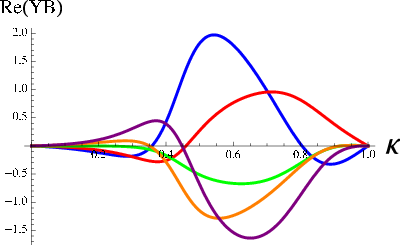
Refer to caption Refer to caption
S​U​(2)RSU(2)_{R} sector S​U​(2)LSU(2)_{L} sector
Figure 5: The figure shows the differences between the left and right-hand sides of the five Yang-Baxter equations, as a function of κ\kappa, for the specific choice of momenta p1=0.3p_{1}=0.3, p2=0.8p_{2}=0.8 and p3=1.4p_{3}=1.4. The blue, red, green, orange and purple curves show (l.h.s)−-(r.h.s) for the the first to fifth equation.

Ordinarily, verification of the Yang-Baxter equation for the two-magnon S-matrix counts as strong evidence for integrability. In our case, however, for κ\kappa strictly zero, the elementary QQ impurities “freeze”, and only Q​Q¯Q\bar{Q} dimers can propagate on the chain. Correspondingly, the QQ dispersion relation becomes momentum-independent,

EQ​(p,κ)=2​(1−κ)2+8​κ​sin2⁡(p2)→κ→02,E_{Q}(p;\kappa)=2(1-\kappa)^{2}+8\kappa\,\sin^{2}(\frac{p}{2})\xrightarrow[\kappa\to 0]{}2\,, (145)

and the S-matrix also degenerates to a simple expression. Verification of YB strictly at κ=0\kappa=0 may then appear like an accident due to this degenerate limit. What we find more significant, and non-trivial evidence for integrability, is that the integrable point κ=0\kappa=0 is reached smoothly, with YB failing infinitesimally for infinitesimal κ\kappa – this is clear since the S-matrices are analytic (rational) functions of κ\kappa. This smooth behavior is illustrated in figure 5, where we plot the differences between the left and right hand sides of the five equations (140–144) (for some choice of the momenta).

An elegant way to conclusively prove one-loop integrability at κ=0\kappa=0 would be to exhibit the algebraic Bethe ansatz for the SCQCD spin chain. The simplest guess for the R-matrix does not appear to work [32], but the issue deserves further investigation.

Another possible approach is to assume integrability to derive Bethe equations for the periodic chain, and then check whether their (numerical) solutions agree with the solutions obtained by direct diagonalization of the Hamiltonian. This is not entirely straightforward, because we cannot work strictly at κ=0\kappa=0. The naive Bethe equations at κ=0\kappa=0 have no interesting solutions for finite values of the Bethe roots – the non-trivial dynamics is hidden in Bethe roots with infinite imaginary parts (in the momentum variable). We saw this phenomenon in the evolution of the bound states as κ→0\kappa\to 0, where the individual magnon momenta behave as i​log⁡κi\log\kappa. Taking the SCQCD limit κ→0\kappa\to 0 too early we lose information about the bound states. (It is conceivable that the failure of the (simplest) algebraic Bethe ansatz is also due to this order-of-limits issue.) Nevertheless, it makes sense to write Bethe equations for small κ\kappa, viewed as a regulator to be removed at the end of the calculation. We can also calculate the S-matrix of the bound states, by using the fusion procedure for infinitesimal κ\kappa, and check their YB equation in the SCQCD limit. The consistency of this approach should follow from the smoothness of the κ→0\kappa\to 0 limit.

A natural extension of our work is the calculation of one-loop dilation operator in the complete theory, including fermions and derivatives [33]. Let us briefly comment on the symmetry structure of the complete spin chain. As is well-known, the symmetry of the 𝒩=4{\cal N}=4 spin chain in the excitation picture is P​S​U​(2|2)L×P​S​U​(2|2)R×ℝPSU(2|2)_{L}\times PSU(2|2)_{R}\times\mathbb{R}, where the central factor ℝ\mathbb{R} is identified with the Hamiltonian. The ℤ2\mathbb{Z}_{2} orbifold projection preserves the P​S​U​(2|2)RPSU(2|2)_{R} in the “right” sector (this is a subgroup of the 𝒩=2{\cal N}=2 superconformal group S​U​(2,2|2)SU(2,2|2)), but breaks P​S​U​(2|2)LPSU(2|2)_{L} to the bosonic subgroup S​U​(2)L×S​U​(2)αSU(2)_{L}\times SU(2)_{\alpha}, where S​U​(2)αSU(2)_{\alpha} denotes the left-handed Lorentz symmetry. At the orbifold point κ=1\kappa=1, the breaking is only due to a global twist of the chain, while locally the symmetry is the same as in 𝒩=4{\cal N}=4, but for κ≠1\kappa\neq 1 the symmetry is truly broken. All in all, the symmetry of the spin chain of the interpolating theory is S​U​(2)L×S​U​(2)α×P​S​U​(2|2)R×ℝSU(2)_{L}\times SU(2)_{\alpha}\times PSU(2|2)_{R}\times\mathbb{R}. In this paper we have found that in the two-body S-matrix of QQ impurities has a left ×\times right factorization, and we expect this feature to persist for the full chain.

An obvious question is whether symmetry is sufficient to fix the form of the S-matrix, as it does to all loops in 𝒩=4{\cal N}=4 SYM (up to an overall scalar factor). While unlikely for SLS_{L}, this is likely for SRS_{R}, which has a large supergroup symmetry. In fact, the symmetry in the right sector of the interpolating SCFT the same as in (either sector of) 𝒩=4{\cal N}=4 SYM. The SRS_{R} matrix of 𝒩=4{\cal N}=4 is uniquely fixed, up to an overall scalar factor, from the (centrally extended) S​U​(2|2)RSU(2|2)_{R} symmetry [34]. But our results for SRS_{R} in the interpolating theory are definitely different (for κ≠1\kappa\neq 1) from the 𝒩=4{\cal N}=4 results. This is clear already in the scalar sector studied in this paper, by inspection of the S-matrix of the Qℐ​+^Q_{{\cal I}\hat{+}} impurities. This discrepancy is explained by the fact in our case the magnons transform in a reducible representation of SU(2|2) (two copies of the fundamental representation). It will be interesting to see whether these assumptions can be relaxed to reproduce (and possibly uniquely fix) Remarkably, it is still possible to use symmetry to fix uniquely the form of the SRS_{R} matrix in the interpolating theory, up to a free parameter that can be identified with κ\kappa. This analysis will be presented elsewhere [35].

Finally it would be very interesting to evaluate the two-body S-matrix at strong coupling, in the dual string sigma-model, and see whether it has the same κ\kappa dependence as the perturbative S-matrix. Failure of integrability for generic κ\kappa is not an issue here, since we would not be using in any way factorization of nn-body scattering, but rather focus on the two-body S-matrix, which we expect to have a smooth interpolation from weak to strong coupling. The sigma-model at the orbifold point is well-known, and moving away from the orbifold point corresponds to changing the value of a theta angle β\beta (the period of the NSNS BB-field through the collapsed cycle of the orbifold) [36, 37]. The orbifold point corresponds to β=1/2\beta=1/2, while the SCQCD limit corresponds to β→0\beta\to 0. From the dual side, it is natural to expect integrability precisely at the two extrema 0 and 1/2, but not for generic values of the BB-field. A toy model for this behavior is the O⁡(3)O(3) sigma-model in a magnetic field [38].

One of our original motivations was to collect “bottom-up” clues about the string dual of 𝒩=2{\cal N}=2 SCQCD. While firm conclusions will have to wait a higher-oder (all order?) analysis, we can already see a qualitative agreement with the “top-down” approach of our previous paper [1]. We argued that 𝒩=2{\cal N}=2 SCQCD is dual to a non-critical string background, with seven geometric dimensions, containing both an A​d​S5AdS_{5} and an S1S^{1} factor. Rotation in S1S^{1} corresponds to the U​(1)rU(1)_{r} quantum number. In lightcone quantization of the sigma-model, the lightcone coordinates would be obtained by combining this S1S^{1} and the timelike direction of A​d​S5AdS_{5}. We then expect five bosonic gapless excitations, four associated to the transverse AdS coordinates and one to the seventh dimension. The vacuum of the lightcone sigma-model corresponds to chiral vacuum Tr​ϕℓ{\rm Tr}\,\phi^{\ell} of the spin chain, while the four AdS excitations correspond to derivative impurities on the chain. In the scalar sector that we have studied in this paper, one gapless excitation is then expected, the one corresponding to the seventh dimension: just what we found, the gapless magnon T⁡(p)T(p). As κ→0\kappa\to 0, the QQ impurities, carriers of the S​U​(2)L×S​U​(2)RSU(2)_{L}\times SU(2)_{R} quantum numbers associated with the three extra dimensions (the transverse S3S^{3}, see [1] for details), become non-dynamical, and only their composite bound state T⁡(p)T(p) survives as a gapless mode. We interpret this phenomenon as the field theory counterpart of the transition from the critical to the non-critical background.

Acknowledgements

It is a pleasure thank Vladimir Korepin, Pedro Liendo, Juan Maldacena, Joe Minahan, Joe Polchinski, Soo-Jong Rey, Martin Rocek, Radu Roiban, Matthias Staudacher, Pedro Vieira, and Kostya Zarembo for useful discussions. This work was supported in part by DOE grant DEFG-0292-ER40697 and by NSF grant PHY-0653351-001. Any opinions, findings, and conclusions or recommendations expressed in this material are those of the authors and do not necessarily reflect the views of the National Science Foundation.

Appendix A Simplified computation of the one-loop dilation operator

In this appendix we determine the one-loop spin-chain Hamiltonian by a simple shortcut. The interactions contributing to Hk,k+1H_{k,k+1} at one loop are listed schematically in figure 1. The first and second interactions (self-energy and gluon exchange) in figure 1 are proportional to the identity operator in Vk⊗Vk+1V_{k}\otimes V_{k+1}, while the non-trivial tensorial structures are contributed only by the third diagram (quartic interaction). The idea is to evaluate explicitly the third diagram, and to fix the terms proportional to the identity by requiring that the anomalous dimensions of a few protected operators vanish.

A.1 SCQCD

Let us recall our notations. The indices 𝔭,𝔮=±\mathfrak{p},\mathfrak{q}=\pm label the U​(1)rU(1)_{r} charges of ϕ\phi and ϕ¯\bar{\phi}, in other terms we define ϕ−≡ϕ\phi^{-}\equiv\phi, ϕ+≡ϕ¯\phi^{+}\equiv\bar{\phi}, and g𝔭​𝔮=(0110)g_{\mathfrak{p}\mathfrak{q}}=\left(\begin{array}[]{cc}0&1\\ 1&0\end{array}\right). The elements of the Hamiltonian due to quartic vertices are:

⟨ϕ𝔭′​ϕ𝔮′|H|ϕ𝔭​ϕ𝔮⟩ϕ4\displaystyle\langle\phi_{\mathfrak{p}^{\prime}}\phi_{\mathfrak{q}^{\prime}}|H|\phi^{\mathfrak{p}}\phi^{\mathfrak{q}}\rangle_{\phi^{4}} =\displaystyle= δ𝔭′𝔭​δ𝔮′𝔮+g𝔭​𝔮​g𝔭′​𝔮′−2​δ𝔮′𝔭​δ𝔭′𝔮\displaystyle\delta_{\mathfrak{p}^{\prime}}^{\mathfrak{p}}\delta_{\mathfrak{q}^{\prime}}^{\mathfrak{q}}+g^{\mathfrak{p}\mathfrak{q}}g_{\mathfrak{p}^{\prime}\mathfrak{q}^{\prime}}-2\delta_{\mathfrak{q}^{\prime}}^{\mathfrak{p}}\delta_{\mathfrak{p}^{\prime}}^{\mathfrak{q}} (146)
⟨ϕ𝔭′​ϕ𝔮′|H|Qℐ​Q¯𝒥⟩Q2​ϕ2\displaystyle\langle\phi_{\mathfrak{p}^{\prime}}\phi_{\mathfrak{q}^{\prime}}|H|Q_{\mathcal{I}}\bar{Q}^{\mathcal{J}}\rangle_{Q^{2}\phi^{2}} =\displaystyle= NfNc​g𝔭′​𝔮′​δℐ𝒥\displaystyle\sqrt{\frac{N_{f}}{N_{c}}}g_{\mathfrak{p}^{\prime}\mathfrak{q}^{\prime}}\delta_{\mathcal{I}}^{\mathcal{J}} (147)
⟨Q¯ℐ′​Q𝒥′|H|Qℐ​Q¯𝒥⟩Q4\displaystyle\langle\bar{Q}^{\mathcal{I}^{\prime}}Q_{\mathcal{J}^{\prime}}|H|Q_{\mathcal{I}}\bar{Q}^{\mathcal{J}}\rangle_{Q^{4}} =\displaystyle= NfNc​(2​δℐℐ′​δ𝒥′𝒥−δℐ𝒥​δ𝒥′ℐ′)\displaystyle\frac{N_{f}}{N_{c}}(2\delta_{\mathcal{I}}^{\mathcal{I}^{\prime}}\delta_{\mathcal{J}^{\prime}}^{\mathcal{J}}-\delta_{\mathcal{I}}^{\mathcal{J}}\delta_{\mathcal{J}^{\prime}}^{\mathcal{I}^{\prime}}) (148)
⟨Q𝒥′​Q¯ℐ′|H|Q¯𝒥​Qℐ⟩Q4\displaystyle\langle Q_{\mathcal{J}^{\prime}}\bar{Q}^{\mathcal{I}^{\prime}}|H|\bar{Q}^{\mathcal{J}}Q_{\mathcal{I}}\rangle_{Q^{4}} =\displaystyle= 2​δℐ𝒥​δ𝒥′ℐ′−δℐℐ′​δ𝒥′𝒥\displaystyle 2\delta_{\mathcal{I}}^{\mathcal{J}}\delta_{\mathcal{J}^{\prime}}^{\mathcal{I}^{\prime}}-\delta_{\mathcal{I}}^{\mathcal{I}^{\prime}}\delta_{\mathcal{J}^{\prime}}^{\mathcal{J}} (149)

The factors of NfNc\frac{N_{f}}{N_{c}} are explained in figure 6. Figures 6a,6b,6c,6d correspond to equations (146,147,148,149) respectively. This fixes the Hamiltonian up to the terms proportional to the identity,

Hk,k+1=\displaystyle H_{k,k+1}=
ϕ𝔭​ϕ𝔮Qℐ​Q¯𝒥Q¯𝒦​QℒQℐ​ϕ𝔭( ) ϕ𝔭′​ϕ𝔮′α​δ𝔭′𝔭​δ𝔮′𝔮+g𝔭​𝔮​g𝔭′​𝔮′−2​δ𝔮′𝔭​δ𝔭′𝔮NfNc​g𝔭′​𝔮′​δℐ𝒥00Q¯ℐ′​Q𝒥′NfNc​g𝔭​𝔮​δ𝒥′ℐ′β​δℐℐ′​δ𝒥′𝒥−δℐ𝒥​δ𝒥′ℐ′​NfNc00Q𝒦′​Q¯ℒ′00γ​δ𝒦′𝒦​δℒℒ′+2​δℒ𝒦​δ𝒦′ℒ′0Q¯ℐ′​ϕ𝔭′000η​δℐℐ′​δ𝔭′𝔭\displaystyle\bordermatrix{&\phi^{\mathfrak{p}}\phi^{\mathfrak{q}}&Q_{\mathcal{I}}\bar{Q}^{\mathcal{J}}&\bar{Q}^{\mathcal{K}}Q_{\mathcal{L}}&Q_{\mathcal{I}}\phi^{\mathfrak{p}}\cr&&&&\cr\phi_{\mathfrak{p}^{\prime}}\phi_{\mathfrak{q}^{\prime}}&\alpha\delta_{\mathfrak{p}^{\prime}}^{\mathfrak{p}}\delta_{\mathfrak{q}^{\prime}}^{\mathfrak{q}}+g^{\mathfrak{p}\mathfrak{q}}g_{\mathfrak{p}^{\prime}\mathfrak{q}^{\prime}}-2\delta_{\mathfrak{q}^{\prime}}^{\mathfrak{p}}\delta_{\mathfrak{p}^{\prime}}^{\mathfrak{q}}&\sqrt{\frac{N_{f}}{N_{c}}}g_{\mathfrak{p}^{\prime}\mathfrak{q}^{\prime}}\delta_{\mathcal{I}}^{\mathcal{J}}&0&0\cr\bar{Q}^{\mathcal{I}^{\prime}}Q_{\mathcal{J}^{\prime}}&\sqrt{\frac{N_{f}}{N_{c}}}g^{\mathfrak{p}\mathfrak{q}}\delta_{\mathcal{J}^{\prime}}^{\mathcal{I}^{\prime}}&\beta\delta_{\mathcal{I}}^{\mathcal{I}^{\prime}}\delta_{\mathcal{J}^{\prime}}^{\mathcal{J}}-\delta_{\mathcal{I}}^{\mathcal{J}}\delta_{\mathcal{J}^{\prime}}^{\mathcal{I}^{\prime}}\frac{N_{f}}{N_{c}}&0&0\cr Q_{\mathcal{K}^{\prime}}\bar{Q}^{\mathcal{L}^{\prime}}&0&0&\gamma\delta_{\mathcal{K}^{\prime}}^{\mathcal{K}}\delta^{\mathcal{L}^{\prime}}_{\mathcal{L}}+2\delta_{\mathcal{L}}^{\mathcal{K}}\delta_{\mathcal{K}^{\prime}}^{\mathcal{L}^{\prime}}&0\cr\bar{Q}^{\mathcal{I}^{\prime}}\phi_{\mathfrak{p}^{\prime}}&0&0&0&\eta\delta_{\mathcal{I}}^{\mathcal{I}^{\prime}}\delta_{\mathfrak{p}^{\prime}}^{\mathfrak{p}}}
Refer to caption

(a)
Refer to caption

(b)
Refer to caption

(c)
Refer to caption
(d)
Figure 6: The color/flavor structure of the quartic vertex. The solid black line represents the flow of the color index while the dotted blue line show the flow of the flavor index. Diagram (a) shows the ϕ4\phi^{4} interaction vertex, whose contribution is proportional to NcN_{c} as compared to the tree level. In (b) the Q2​ϕ2Q^{2}\phi^{2} interaction vertex has a factor of Nf/NcN_{f}/N_{c} compared to (a) because of the presence of one flavor loop. The Q4Q^{4} vertex in (c) has an additional factor of (Nf/Nc)2(N_{f}/N_{c})^{2} compared to (a) due to the presence of two flavor loops. Diagram (d), however, does not carry any additional Nf/NcN_{f}/N_{c} factors.

We can now find the coefficients α,β,γ\alpha,\beta,\gamma and η\eta from knowledge of the protected spectrum. Vanishing of the anomalous dimension of Tr​ϕk\mbox{Tr}\phi^{k} gives α=2\alpha=2. Another protected multiplet is the multiplet containing the stress-energy tensor. Its superconformal primary, called Tr​T\mbox{Tr}\,T, has R,r=0R,r=0 and Δ=2\Delta=2. Hence, it is a linear combination of Tr​[Qℐ​Q¯ℐ]\mbox{Tr}[Q_{\mathcal{I}}\bar{Q}^{\mathcal{I}}] and Tr​[ϕ​ϕ¯]\mbox{Tr}[\phi\bar{\phi}]. The restriction of the Hamiltonian to this subspace is

H=Tr​[ϕ​ϕ¯]Tr​[ℳ𝟏]Tr​[ϕ​ϕ¯]( 42​2​NfN) Tr​[ℳ𝟏]2​2​NfN(β+γ)−2​(NfNc−2)H=\quad\bordermatrix{&\mbox{Tr}[\phi\bar{\phi}]&&\mbox{Tr}[\mathcal{M}_{\bf 1}]\cr\mbox{Tr}[\phi\bar{\phi}]&4&&2\sqrt{\frac{2N_{f}}{N}}\cr\mbox{Tr}[\mathcal{M}_{\bf 1}]&2\sqrt{\frac{2N_{f}}{N}}&&(\beta+\gamma)-2(\frac{N_{f}}{N_{c}}-2)} (150)

This matrix must have a zero at the superconformal point Nf=2​NcN_{f}=2N_{c}, yielding β+γ=4\beta+\gamma=4. Finally, the fact that Tr​T​ϕ\mbox{Tr}\,T\phi is also a protected operator gives the relation β+2​η=8\beta+2\eta=8. We started with four coefficients α\alpha, β\beta, γ\gamma, η\eta and imposed three relations. The undetermined degrees of freedom corresponds to the “gauge” freedom of adding to the nearest neighbor Hamiltonian terms that vanish upon evaluating the full HH on a closed chain. We may solve the constraints by writing

α=2,β=4+12​(1+ξ),γ=−12​(1+ξ),η=14​(7−ξ),\alpha=2\,,\qquad\beta=4+\frac{1}{2}(1+\xi)\,,\qquad\gamma=-\frac{1}{2}(1+\xi)\,,\qquad\eta=\frac{1}{4}(7-\xi)\,, (151)

where ξ\xi is the arbitrary gauge parameter. The resulting Hamiltonian is in perfect agreement (for Nf=2​NcN_{f}=2N_{c}) with the answer (35) obtained by the slightly lengthier route of explicit evaluating all relevant one-loop diagrams. All in all, this confirms our understanding of the protected spectrum.

A.2 Interpolating SCFT

We can repeat the same exercise for the interpolating SCFT. The quartic vertices give

⟨ϕ𝔭′​ϕ𝔮′|ϕ𝔭​ϕ𝔮⟩ϕ4\displaystyle\langle\phi_{\mathfrak{p}^{\prime}}\phi_{\mathfrak{q}^{\prime}}|\phi^{\mathfrak{p}}\phi^{\mathfrak{q}}\rangle_{\phi^{4}} =\displaystyle= δ𝔭′𝔭​δ𝔮′𝔮+g𝔭​𝔮​g𝔭′​𝔮′−2​δ𝔮′𝔭​δ𝔭′𝔮\displaystyle\delta_{\mathfrak{p}^{\prime}}^{\mathfrak{p}}\delta_{\mathfrak{q}^{\prime}}^{\mathfrak{q}}+g^{\mathfrak{p}\mathfrak{q}}g_{\mathfrak{p}^{\prime}\mathfrak{q}^{\prime}}-2\delta_{\mathfrak{q}^{\prime}}^{\mathfrak{p}}\delta_{\mathfrak{p}^{\prime}}^{\mathfrak{q}} (152)
⟨ϕˇ𝔭′​ϕˇ𝔮′|ϕˇ𝔭​ϕˇ𝔮⟩ϕˇ4\displaystyle\langle\check{\phi}_{\mathfrak{p}^{\prime}}\check{\phi}_{\mathfrak{q}^{\prime}}|\check{\phi}^{\mathfrak{p}}\check{\phi}^{\mathfrak{q}}\rangle_{\check{\phi}^{4}} =\displaystyle= κ2​(δ𝔭′𝔭​δ𝔮′𝔮+g𝔭​𝔮​g𝔭′​𝔮′−2​δ𝔮′𝔭​δ𝔭′𝔮)\displaystyle\kappa^{2}(\delta_{\mathfrak{p}^{\prime}}^{\mathfrak{p}}\delta_{\mathfrak{q}^{\prime}}^{\mathfrak{q}}+g^{\mathfrak{p}\mathfrak{q}}g_{\mathfrak{p}^{\prime}\mathfrak{q}^{\prime}}-2\delta_{\mathfrak{q}^{\prime}}^{\mathfrak{p}}\delta_{\mathfrak{p}^{\prime}}^{\mathfrak{q}}) (153)
⟨Q¯ℒ^​ℒ​Q𝒦​𝒦^|Qℐ​ℐ^​Q¯𝒥^​𝒥⟩Q4\displaystyle\langle\bar{Q}^{\hat{\mathcal{L}}\mathcal{L}}Q_{\mathcal{K}\hat{\mathcal{K}}}|Q_{\mathcal{I}\hat{\mathcal{I}}}\bar{Q}^{\hat{\mathcal{J}}\mathcal{J}}\rangle_{Q^{4}} =\displaystyle= 2​δℐ^𝒥^​δ𝒦𝒥​δ𝒦^ℒ^​δℐℒ−δℐ𝒥​δℐ^𝒥^​δ𝒦ℒ​δ𝒦^ℒ^\displaystyle 2\,\delta_{\hat{\mathcal{I}}}^{\hat{\mathcal{J}}}\delta_{\mathcal{K}}^{\mathcal{J}}\delta_{\hat{\mathcal{K}}}^{\hat{\mathcal{L}}}\delta_{\mathcal{I}}^{\mathcal{L}}-\delta_{\mathcal{I}}^{\mathcal{J}}\delta_{\hat{\mathcal{I}}}^{\hat{\mathcal{J}}}\delta_{\mathcal{K}}^{\mathcal{L}}\delta_{\hat{\mathcal{K}}}^{\hat{\mathcal{L}}} (154)
+\displaystyle+ κ2​(2​δ𝒦^𝒥^​δℐ𝒥​δℐ^ℒ^​δ𝒦ℒ−δℐℒ​δℐ^ℒ^​δ𝒦𝒥​δ𝒦^𝒥^)\displaystyle\kappa^{2}(2\,\delta_{\hat{\mathcal{K}}}^{\hat{\mathcal{J}}}\delta_{\mathcal{I}}^{\mathcal{J}}\delta_{\hat{\mathcal{I}}}^{\hat{\mathcal{L}}}\delta_{\mathcal{K}}^{\mathcal{L}}-\delta_{\mathcal{I}}^{\mathcal{L}}\delta_{\hat{\mathcal{I}}}^{\hat{\mathcal{L}}}\delta_{\mathcal{K}}^{\mathcal{J}}\delta_{\hat{\mathcal{K}}}^{\hat{\mathcal{J}}})
⟨Qℐ​ℐ^​Q¯𝒥^​𝒥|Q¯ℒ^​ℒ​Q𝒦​𝒦^⟩Q4\displaystyle\langle Q_{\mathcal{I}\hat{\mathcal{I}}}\bar{Q}^{\hat{\mathcal{J}}\mathcal{J}}|\bar{Q}^{\hat{\mathcal{L}}\mathcal{L}}Q_{\mathcal{K}\hat{\mathcal{K}}}\rangle_{Q^{4}} =\displaystyle= 2​δℐ^𝒥^​δ𝒦𝒥​δ𝒦^ℒ^​δℐℒ−δℐ𝒥​δℐ^𝒥^​δ𝒦ℒ​δ𝒦^ℒ^\displaystyle 2\,\delta_{\hat{\mathcal{I}}}^{\hat{\mathcal{J}}}\delta_{\mathcal{K}}^{\mathcal{J}}\delta_{\hat{\mathcal{K}}}^{\hat{\mathcal{L}}}\delta_{\mathcal{I}}^{\mathcal{L}}-\delta_{\mathcal{I}}^{\mathcal{J}}\delta_{\hat{\mathcal{I}}}^{\hat{\mathcal{J}}}\delta_{\mathcal{K}}^{\mathcal{L}}\delta_{\hat{\mathcal{K}}}^{\hat{\mathcal{L}}} (155)
+\displaystyle+ κ2​(2​δ𝒦^𝒥^​δℐ𝒥​δℐ^ℒ^​δ𝒦ℒ−δℐℒ​δℐ^ℒ^​δ𝒦𝒥​δ𝒦^𝒥^)\displaystyle\kappa^{2}(2\,\delta_{\hat{\mathcal{K}}}^{\hat{\mathcal{J}}}\delta_{\mathcal{I}}^{\mathcal{J}}\delta_{\hat{\mathcal{I}}}^{\hat{\mathcal{L}}}\delta_{\mathcal{K}}^{\mathcal{L}}-\delta_{\mathcal{I}}^{\mathcal{L}}\delta_{\hat{\mathcal{I}}}^{\hat{\mathcal{L}}}\delta_{\mathcal{K}}^{\mathcal{J}}\delta_{\hat{\mathcal{K}}}^{\hat{\mathcal{J}}})
⟨ϕ𝔭′​ϕ𝔮′|Qℐ​ℐ^​Q¯𝒥^​𝒥⟩Q2​ϕ2\displaystyle\langle\phi_{\mathfrak{p}^{\prime}}\phi_{\mathfrak{q}^{\prime}}|Q_{\mathcal{I}\hat{\mathcal{I}}}\bar{Q}^{\hat{\mathcal{J}}\mathcal{J}}\rangle_{Q^{2}\phi^{2}} =\displaystyle= g𝔭′​𝔮′​δℐ𝒥​δℐ^𝒥^\displaystyle g_{\mathfrak{p}^{\prime}\mathfrak{q}^{\prime}}\delta_{\mathcal{I}}^{\mathcal{J}}\delta_{\hat{\mathcal{I}}}^{\hat{\mathcal{J}}} (156)
⟨ϕˇ𝔭′​ϕˇ𝔮′|Q¯𝒥^​𝒥​Qℐ​ℐ^⟩Q2​ϕˇ2\displaystyle\langle\check{\phi}_{\mathfrak{p}^{\prime}}\check{\phi}_{\mathfrak{q}^{\prime}}|\bar{Q}^{\hat{\mathcal{J}}\mathcal{J}}Q_{\mathcal{I}\hat{\mathcal{I}}}\rangle_{Q^{2}\check{\phi}^{2}} =\displaystyle= κ2​g𝔭′​𝔮′​δℐ𝒥​δℐ^𝒥^\displaystyle\kappa^{2}g_{\mathfrak{p}^{\prime}\mathfrak{q}^{\prime}}\delta_{\mathcal{I}}^{\mathcal{J}}\delta_{\hat{\mathcal{I}}}^{\hat{\mathcal{J}}} (157)
⟨Q¯𝒥^​𝒥​ϕˇ𝔮|ϕ𝔭​Qℐ​ℐ^⟩ϕ​Q​ϕˇ​Q¯\displaystyle\langle\bar{Q}^{\hat{\mathcal{J}}\mathcal{J}}\check{\phi}_{\mathfrak{q}}|\phi^{\mathfrak{p}}Q_{\mathcal{I}\hat{\mathcal{I}}}\rangle_{\phi Q\check{\phi}\bar{Q}} =\displaystyle= −2​κ​δ𝔮𝔭​δℐ𝒥​δℐ^𝒥^\displaystyle-2\kappa\delta_{\mathfrak{q}}^{\mathfrak{p}}\delta_{\mathcal{I}}^{\mathcal{J}}\delta_{\hat{\mathcal{I}}}^{\hat{\mathcal{J}}} (158)
⟨ϕ𝔭​Q¯𝒥^​𝒥|Qℐ​ℐ^​ϕˇ𝔮⟩ϕ​Q​ϕˇ​Q¯\displaystyle\langle\phi^{\mathfrak{p}}\bar{Q}^{\hat{\mathcal{J}}\mathcal{J}}|Q_{\mathcal{I}\hat{\mathcal{I}}}\check{\phi}_{\mathfrak{q}}\rangle_{\phi Q\check{\phi}\bar{Q}} =\displaystyle= −2​κ​δ𝔮𝔭​δℐ𝒥​δℐ^𝒥^\displaystyle-2\kappa\delta_{\mathfrak{q}}^{\mathfrak{p}}\delta_{\mathcal{I}}^{\mathcal{J}}\delta_{\hat{\mathcal{I}}}^{\hat{\mathcal{J}}} (159)

The first four elements can have additional identity pieces. They are easily determined by imposing the symmetry under g↔gˇg\leftrightarrow\check{g}, Q↔Q¯Q\leftrightarrow\bar{Q} and ϕ↔ϕˇ\phi\leftrightarrow\check{\phi} and by requiring the Hamiltonian to reduce to that of SCQCD in the limit κ→0\kappa\to 0. The one loop Hamiltonian (54) is precisely reproduced by this method.

Appendix B The Hamiltonian for SCQCD in the Dimer Picture

In this appendix we rewrite the Hamiltonian for SCQCD as acting on adjoint fields and dimers Qℐ​Q¯𝒥Q_{\mathcal{I}}\bar{Q}^{\mathcal{J}}, regarded as basic objects. We define the singlet combination ℳ=12ℳℐ 𝒥δ𝒥ℐ\mathcal{M}=\frac{1}{\sqrt{2}}\mathcal{M}_{\mathcal{I}}^{\mbox{ }\mathcal{J}}\delta_{\mathcal{J}}^{\mathcal{I}} and the triplet ℳi=12ℳℐ 𝒥(σi)𝒥ℐ\mathcal{M}^{i}=\frac{1}{\sqrt{2}}\mathcal{M}_{\mathcal{I}}^{\mbox{ }\mathcal{J}}(\sigma^{i})_{\mathcal{J}}^{\mathcal{I}}, where σi\sigma^{i} are three Pauli matrices. These can be rewritten in an S​O​(4)SO(4) notation as ℳm=12ℳℐ 𝒥(σm)𝒥ℐ\mathcal{M}^{m}=\frac{1}{\sqrt{2}}\mathcal{M}_{\mathcal{I}}^{\mbox{ }\mathcal{J}}(\sigma^{m})_{\mathcal{J}}^{\mathcal{I}}, where m=0,…,3m=0,\ldots,3 and σ0≡𝕀2×2\sigma^{0}\equiv\mathbb{I}_{2\times 2}.

Consider the action of HH on following sequence in the spin chain,

ϕ𝔭QℐQ¯𝒥ϕ𝔮12​(3+ξ2)(5−ξ2)​𝕀Q​Q−2​𝕂Q​Q12​(3+ξ2)↓↓↓ϕ𝔭′Q¯ℐ′Q𝒥′ϕ𝔮′\begin{array}[]{ccccccc}\phi^{\mathfrak{p}}&&Q_{\mathcal{I}}&&\bar{Q}^{\mathcal{J}}&&\phi^{\mathfrak{q}}\\ &\frac{1}{2}(3+\frac{\xi}{2})&&(5-\frac{\xi}{2})\mathbb{I}_{QQ}-2\mathbb{K}_{QQ}&&\frac{1}{2}(3+\frac{\xi}{2})\\ &\downarrow&&\downarrow&&\downarrow\\ \phi_{\mathfrak{p}^{\prime}}&&\bar{Q}^{\mathcal{I}^{\prime}}&&Q_{\mathcal{J}^{\prime}}&&\phi_{\mathfrak{q}^{\prime}}\end{array} (160)

In the new picture, where ℳ\mathcal{M} is regarded as a basic impurity, the middle term (5−ξ2)​𝕀Q​Q−2​𝕂Q​Q(5-\frac{\xi}{2})\mathbb{I}_{QQ}-2\mathbb{K}_{QQ} is the “self energy” of ℳ\mathcal{M}, and we split it evenly between the ϕ​ℳ\phi{\cal M} and ℳ​ϕ{\cal M}\phi matrix elements. So we write

⟨…ϕ𝔭′ℳ¯ 𝒥′ℐ′…|H|…ϕ𝔭ℳℐ 𝒥…⟩\displaystyle\langle\ldots\phi_{\mathfrak{p}^{\prime}}\bar{\mathcal{M}}_{\mbox{ }\mathcal{J}^{\prime}}^{\mathcal{I}^{\prime}}\ldots|H|\ldots\phi^{\mathfrak{p}}\mathcal{M}_{\mathcal{I}}^{\mbox{ }\mathcal{J}}\ldots\rangle =\displaystyle= [12​(3+ξ2)+12​(5−ξ2)]​δ𝔭′𝔭​δℐℐ′​δ𝒥′𝒥−δ𝔭′𝔭​δℐ𝒥​δ𝒥′ℐ′\displaystyle[\frac{1}{2}(3+\frac{\xi}{2})+\frac{1}{2}(5-\frac{\xi}{2})]\delta_{\mathfrak{p}^{\prime}}^{\mathfrak{p}}\delta_{\mathcal{I}}^{\mathcal{I}^{\prime}}\delta_{\mathcal{J}^{\prime}}^{\mathcal{J}}-\delta_{\mathfrak{p}^{\prime}}^{\mathfrak{p}}\delta_{\mathcal{I}}^{\mathcal{J}}\delta_{\mathcal{J}^{\prime}}^{\mathcal{I}^{\prime}}
=\displaystyle= (4​δℐℐ′​δ𝒥′𝒥−δℐ𝒥​δ𝒥′ℐ′)​δ𝔭′𝔭\displaystyle(4\delta_{\mathcal{I}}^{\mathcal{I}^{\prime}}\delta_{\mathcal{J}^{\prime}}^{\mathcal{J}}-\delta_{\mathcal{I}}^{\mathcal{J}}\delta_{\mathcal{J}^{\prime}}^{\mathcal{I}^{\prime}})\delta_{\mathfrak{p}^{\prime}}^{\mathfrak{p}}
⟨…​ϕ𝔭′​ℳ¯m′​…|H|…​ϕ𝔭​ℳm​…⟩\displaystyle\langle\ldots\phi_{\mathfrak{p}^{\prime}}\bar{\mathcal{M}}^{m^{\prime}}\ldots|H|\ldots\phi^{\mathfrak{p}}\mathcal{M}^{m}\ldots\rangle =\displaystyle= δ𝔭′𝔭​δm​m′​(4−2​δm​0).\displaystyle\delta_{\mathfrak{p}^{\prime}}^{\mathfrak{p}}\delta^{mm^{\prime}}(4-2\delta^{m0})\,.

Similarly, to find the action of HH on two neighboring ℳ{\cal M}s, we consider the sequence

QℐQ¯𝒥Q𝒦Q¯ℒ(5−ξ2)​𝕀Q​Q−2​𝕂Q​Q(ξ2−1)​𝕀Q​Q+2​𝕂Q​Q(5−ξ2)​𝕀Q​Q−2​𝕂Q​Q↓↓↓Q¯ℐ′Q𝒥′Q¯𝒦′Qℒ′\begin{array}[]{ccccccc}Q_{\mathcal{I}}&&\bar{Q}^{\mathcal{J}}&&Q_{\mathcal{K}}&&\bar{Q}^{\mathcal{L}}\\ &(5-\frac{\xi}{2})\mathbb{I}_{QQ}-2\mathbb{K}_{QQ}&&(\frac{\xi}{2}-1)\mathbb{I}_{QQ}+2\mathbb{K}_{QQ}&&(5-\frac{\xi}{2})\mathbb{I}_{QQ}-2\mathbb{K}_{QQ}\\ &\downarrow&&\downarrow&&\downarrow\\ \bar{Q}^{\mathcal{I}^{\prime}}&&Q_{\mathcal{J}^{\prime}}&&\bar{Q}^{\mathcal{K}^{\prime}}&&Q_{\mathcal{L}^{\prime}}\end{array} (161)

This gives

⟨…​ℳ¯m′​ℳ¯n′​…|H|…​ℳm​ℳn​…⟩\displaystyle\langle\ldots\bar{\mathcal{M}}^{m^{\prime}}\bar{\mathcal{M}}^{n^{\prime}}\ldots|H|\ldots\mathcal{M}^{m}\mathcal{M}^{n}\ldots\rangle =\displaystyle= δm​m′​δn​n′​(13−4​δm​0−4​δn​0)\displaystyle\delta^{mm^{\prime}}\delta^{nn^{\prime}}(13-4\delta^{m0}-4\delta^{n0})
+δm​n​δm′​n′−δm​n′​δn​m′+i​ϵm​n​n′​m′.\displaystyle+\delta^{mn}\delta^{m^{\prime}n^{\prime}}-\delta^{mn^{\prime}}\delta^{nm^{\prime}}+i\epsilon^{mnn^{\prime}m^{\prime}}\,.

References

  • [1] A. Gadde, E. Pomoni, and L. Rastelli, The Veneziano Limit of 𝒩=2{\cal N}=2 Superconformal QCD: Towards the String Dual of 𝒩=2{\cal N}=2 S​U​(Nc)SU(N_{c}) SYM with Nf=2​NcN_{f}=2N_{c}, arXiv:0912.4918.
  • [2] J. A. Minahan and K. Zarembo, The Bethe-ansatz for N = 4 super Yang-Mills, JHEP 03 (2003) 013, [hep-th/0212208].
  • [3] N. Beisert and M. Staudacher, The N=4 SYM Integrable Super Spin Chain, Nucl. Phys. B670 (2003) 439–463, [hep-th/0307042].
  • [4] M. Staudacher, The factorized S-matrix of CFT/AdS, JHEP 05 (2005) 054, [hep-th/0412188].
  • [5] N. Beisert and M. Staudacher, Long-range PSU(2,2|4) Bethe ansaetze for gauge theory and strings, Nucl. Phys. B727 (2005) 1–62, [hep-th/0504190].
  • [6] N. Beisert, B. Eden, and M. Staudacher, Transcendentality and crossing, J. Stat. Mech. 0701 (2007) P021, [hep-th/0610251].
  • [7] N. Gromov, V. Kazakov, and P. Vieira, Exact Spectrum of Anomalous Dimensions of Planar N=4 Supersymmetric Yang-Mills Theory, Phys. Rev. Lett. 103 (2009) 131601, [arXiv:0901.3753].
  • [8] S.-J. Rey and T. Suyama, Exact Results and Holography of Wilson Loops in N=2 Superconformal (Quiver) Gauge Theories, arXiv:1001.0016.
  • [9] G. Veneziano, Some Aspects of a Unified Approach to Gauge, Dual and Gribov Theories, Nucl. Phys. B117 (1976) 519–545.
  • [10] G. ’t Hooft, A planar diagram theory for strong interactions, Nucl. Phys. B72 (1974) 461.
  • [11] J. Kinney, J. M. Maldacena, S. Minwalla, and S. Raju, An index for 4 dimensional super conformal theories, Commun. Math. Phys. 275 (2007) 209–254, [hep-th/0510251].
  • [12] N. Beisert and R. Roiban, The Bethe ansatz for Z(S) orbifolds of N = 4 super Yang- Mills theory, JHEP 11 (2005) 037, [hep-th/0510209].
  • [13] A. Solovyov, Bethe Ansatz Equations for General Orbifolds of N=4 SYM, JHEP 04 (2008) 013, [arXiv:0711.1697].
  • [14] M. R. Douglas and G. W. Moore, D-branes, Quivers, and ALE Instantons, hep-th/9603167.
  • [15] A. Dymarsky, I. R. Klebanov, and R. Roiban, Perturbative gauge theory and closed string tachyons, JHEP 11 (2005) 038, [hep-th/0509132].
  • [16] J. A. Minahan and K. Zarembo, The Bethe ansatz for superconformal Chern-Simons, JHEP 09 (2008) 040, [arXiv:0806.3951].
  • [17] D. Bak and S.-J. Rey, Integrable Spin Chain in Superconformal Chern-Simons Theory, JHEP 10 (2008) 053, [arXiv:0807.2063].
  • [18] D. Gaiotto, S. Giombi, and X. Yin, Spin Chains in N=6 Superconformal Chern-Simons-Matter Theory, JHEP 04 (2009) 066, [arXiv:0806.4589].
  • [19] D. Bak, D. Gang, and S.-J. Rey, Integrable Spin Chain of Superconformal U(M)xU(N) Chern- Simons Theory, JHEP 10 (2008) 038, [arXiv:0808.0170].
  • [20] O. Aharony, O. Bergman, D. L. Jafferis, and J. Maldacena, N=6 superconformal Chern-Simons-matter theories, M2-branes and their gravity duals, JHEP 10 (2008) 091, [arXiv:0806.1218].
  • [21] O. Aharony, O. Bergman, and D. L. Jafferis, Fractional M2-branes, JHEP 11 (2008) 043, [arXiv:0807.4924].
  • [22] J. A. Minahan, W. Schulgin, and K. Zarembo, Two loop integrability for Chern-Simons theories with N=6 supersymmetry, JHEP 03 (2009) 057, [arXiv:0901.1142].
  • [23] J. Minahan, O. Ohlsson Sax, and C. Sieg, Magnon dispersion to four loops in the ABJM and ABJ models, J.Phys.A A43 (2010) 275402, [arXiv:0908.2463].
  • [24] P. Di Vecchia and A. Tanzini, N = 2 super Yang-Mills and the XXZ spin chain, J. Geom. Phys. 54 (2005) 116–130, [hep-th/0405262].
  • [25] V. K. Dobrev and V. B. Petkova, ON THE GROUP THEORETICAL APPROACH TO EXTENDED CONFORMAL SUPERSYMMETRY: CLASSIFICATION OF MULTIPLETS, Lett. Math. Phys. 9 (1985) 287–298.
  • [26] V. K. Dobrev and V. B. Petkova, GROUP THEORETICAL APPROACH TO EXTENDED CONFORMAL SUPERSYMMETRY: FUNCTION SPACE REALIZATIONS AND INVARIANT DIFFERENTIAL OPERATORS, Fortschr. Phys. 35 (1987) 537.
  • [27] V. K. Dobrev and V. B. Petkova, All Positive Energy Unitary Irreducible Representations of Extended Conformal Supersymmetry, Phys. Lett. B162 (1985) 127–132.
  • [28] F. A. Dolan and H. Osborn, On short and semi-short representations for four dimensional superconformal symmetry, Ann. Phys. 307 (2003) 41–89, [hep-th/0209056].
  • [29] V. K. Dobrev, Characters of the positive energy UIRs of D = 4 conformal supersymmetry, Phys. Part. Nucl. 38 (2007) 564–609, [hep-th/0406154].
  • [30] S. Gukov, Comments on N = 2 AdS orbifolds, Phys. Lett. B439 (1998) 23–28, [hep-th/9806180].
  • [31] Y. Nakayama, Index for orbifold quiver gauge theories, Phys. Lett. B636 (2006) 132–136, [hep-th/0512280].
  • [32] A. Gadde and W. Yan, Private Communication, .
  • [33] P. Liendo, E. Pomoni, and L. Rastelli, The Complete One-Loop Dilation Operator of N=2 SuperConformal QCD, arXiv:1105.3972.
  • [34] N. Beisert, The su(2|2) dynamic S-matrix, Adv. Theor. Math. Phys. 12 (2008) 945, [hep-th/0511082].
  • [35] A. Gadde and L. Rastelli, Twisted Magnons, arXiv:1012.2097.
  • [36] A. E. Lawrence, N. Nekrasov, and C. Vafa, On conformal field theories in four dimensions, Nucl. Phys. B533 (1998) 199–209, [hep-th/9803015].
  • [37] I. R. Klebanov and N. A. Nekrasov, Gravity duals of fractional branes and logarithmic RG flow, Nucl. Phys. B574 (2000) 263–274, [hep-th/9911096].
  • [38] A. B. Zamolodchikov and A. B. Zamolodchikov, Massless factorized scattering and sigma models with topological terms, Nucl. Phys. B379 (1992) 602–623.