跳到论文正文
W Papers独立论文阅读器 arXiv:1005.5706 论文正文 计算阅读时间 · 0%
引用这篇论文根据当前论文元数据生成,正式投稿前建议核对。


License: arXiv.org perpetual non-exclusive license
arXiv:1005.5706v2 [hep-ph] 15 Jun 2010

TUM-HEP 762/10
MPP-2010-68

Radiatively induced flavour violation in the general two-Higgs doublet model with Yukawa alignment

Carolin B. Braeuninger★,♥, Alejandro Ibarra★ and Cristoforo Simonetto★

★Physik-Department T30d, Technische Universität München,
James-Franck-Straße, 85748 Garching, Germany

♥Max-Planck-Institut für Physik (Werner-Heisenberg-Institut),
Föhringer Ring 6, 80805 München, Germany

June 14, 2010

The most general two Higgs doublet model contains new sources of flavour violation that are usually in conflict with the experimental constraints. One possibility to suppress the exotic contribution to the flavour changing neutral currents consists on imposing the alignment of the Yukawa couplings. This condition presumably holds at a high-energy scale and is spoiled by the radiative corrections. We compute in this letter the size of the radiatively induced flavour violating Higgs couplings at the electroweak scale. These also yield the absolute lower bound on the size of the exotic contributions to the flavour changing neutral currents in any two Higgs doublet model, barring cancellations and the existence of discrete symmetries. We show that these contributions are well below the experimental bounds in large regions of the parameter space.

1 Introduction

The LHC finally set out to find the Higgs and in anticipation of its results it is important to consider all viable scenarios for the Higgs sector in order to be able to interpret the data once they arrive. The simplest extensions of the SM Higgs sector are so-called two Higgs doublet models (2HDM) where a second Higgs doublet is added to the SM particle content. In addition to the three Goldstone bosons needed to generate the gauge boson masses, there are then five physical Higgs particles: two neutral scalars hh and HH, one neutral pseudo-scalar AA and two charged scalars H±H^{\pm}.

In the most general 2HDM there are two Yukawa matrices per fermion type (up-type quarks, down-type quarks, leptons) which cannot be simultaneously diagonalized. Without any further protection, this leads to unacceptably large flavour changing neutral currents (FCNCs). Therefore in the literature mostly 2HDMs with a discrete symmetry have been considered, ensuring that each right-handed fermion field can couple to no more than one Higgs doublet. There are several choices of the discrete symmetry. The ones most often studied are referred to as type I (only one of the Higgs doublets couples to the fermions) or type II (down-type quarks and leptons couple to one Higgs doublet, up-type quarks to the other) 2HDM. FCNCs are completely absent at tree level in such models.

A generic way to suppress the FCNCs consists in imposing the hypothesis of Minimal Flavour Violation to the flavour symmetry breaking parameters [1]. This hypothesis is implemented in the aligned two-Higgs Doublet model recently discussed in [2]: If the two Yukawa couplings for each fermion type are aligned, they are simultaneously diagonalizable and FCNCs are absent at tree level. This ansatz is more general than discrete symmetries in two ways: Firstly, it contains type I and type II and all other 2HDMs with discrete symmetries as particular cases. Secondly, it allows to have additional sources of CP violation in the Yukawa sector, in contrast to type I and II 2HDM.

The alignment condition presumably holds at a high-energy scale and, in general, will be spoiled by quantum corrections. In this letter we analyse the size of these corrections in order to determine the viability of this scenario. Furthermore, in the absence of cancellations and in the absence of ad hoc discrete symmetries, this scenario yields the lower bound on the exotic contributions to the FCNCs in any 2HDM.

The paper is organized as follows: In sec. 2 we recapitulate the 2HDM and Yukawa alignment. In sec. 3 we present an approximate solution to the renormalization group equations (RGEs) in a 2HDM with Yukawa alignment. Therefrom we derive expressions for the flavour violating neutral Higgs couplings in the quark sector in sec. 4. Bounds on the parameters entering in these couplings are then derived from experimental constraints on meson-antimeson mixing and the leptonic B decay in sec. 5. Finally we conclude in sec. 6.

2 The 2HDM with Yukawa alignment

The general 2HDM we consider has the same fermion content and SU​(3)C×SU​(2)L×U​(1)Y{\rm SU}(3)_{C}\times{\rm SU}(2)_{L}\times{\rm U}(1)_{Y} gauge symmetry as the Standard Model. The Higgs sector consists of two scalar SU⁡(2){\rm SU}(2) doublets ϕ1\phi_{1} and ϕ2\phi_{2} with weak hypercharge Y=12Y=\frac{1}{2}. Both Higgs doublets couple to all fermions11 1 This is sometimes called a type III 2HDM. and the Yukawa part of the Lagrangian therefore reads:

ℒYukawa=(Yu(1))i​j​q¯L​i′​uR​j′​ϕ~1+(Yd(1))i​j​q¯L​i′​dR​j′​ϕ1+(Ye(1))i​j​l¯L​i′​eR​j′​ϕ1+(Yu(2))i​j​q¯L​i′​uR​j′​ϕ~2+(Yd(2))i​j​q¯L​i′​dR​j′​ϕ2+(Ye(2))i​j​l¯L​i′​eR​j′​ϕ2+h.c.\begin{split}\mathcal{L}_{\rm Yukawa}=(Y^{(1)}_{u})_{ij}\bar{q}_{Li}^{\prime}u_{Rj}^{\prime}\tilde{\phi}_{1}+(Y^{(1)}_{d})_{ij}\bar{q}_{Li}^{\prime}d_{Rj}^{\prime}\phi_{1}+(Y^{(1)}_{e})_{ij}\bar{l}_{Li}^{\prime}e_{Rj}^{\prime}\phi_{1}\\ +(Y^{(2)}_{u})_{ij}\bar{q}_{Li}^{\prime}u_{Rj}^{\prime}\tilde{\phi}_{2}+(Y^{(2)}_{d})_{ij}\bar{q}_{Li}^{\prime}d_{Rj}^{\prime}\phi_{2}+(Y^{(2)}_{e})_{ij}\bar{l}_{Li}^{\prime}e_{Rj}^{\prime}\phi_{2}+\rm{h.c.}\end{split} (1)

where i,ji,j are flavour indices and ϕ~a=i​τ2​ϕa∗\tilde{\phi}_{a}=i\tau_{2}\phi^{*}_{a}. The neutral components of the two Higgs doublets acquire vacuum expectation values (vevs) during electroweak symmetry breaking (EWSB) which in general can be complex. While one phase can be rotated away, the phase difference is physical. Nevertheless we can choose to work in a basis where both vevs are positive, shifting the phase to the potential and the Yukawas:

⟨ϕa⟩=12​(0va).\left\langle\phi_{a}\right\rangle=\frac{1}{\sqrt{2}}\left(\begin{array}[]{c}0\\ v_{a}\end{array}\right). (2)

In order to minimize the FCNC effects without imposing ad hoc discrete symmetries we postulate that at a high energy cut-off scale, Λ\Lambda, the Yukawa couplings of the same fermion type are aligned [2]. We parameterize this condition as:

Yu(1)​(Λ)\displaystyle Y_{u}^{(1)}(\Lambda) =cos⁡ψu​Yu,Yu(2)​(Λ)\displaystyle=\cos\psi_{u}Y_{u},\ \ \ \ \ \ Y_{u}^{(2)}(\Lambda) =sin⁡ψu​Yu,\displaystyle=\sin\psi_{u}Y_{u}, (3)
Yd(1)​(Λ)\displaystyle Y_{d}^{(1)}(\Lambda) =cos⁡ψd​Yd,Yd(2)​(Λ)\displaystyle=\cos\psi_{d}Y_{d},\ \ \ \ \ \ Y_{d}^{(2)}(\Lambda) =sin⁡ψd​Yd,\displaystyle=\sin\psi_{d}Y_{d}, (4)
Ye(1)​(Λ)\displaystyle Y_{e}^{(1)}(\Lambda) =cos⁡ψe​Ye,Ye(2)​(Λ)\displaystyle=\cos\psi_{e}Y_{e},\ \ \ \ \ \ Y_{e}^{(2)}(\Lambda) =sin⁡ψe​Ye;\displaystyle=\sin\psi_{e}Y_{e}; (5)

The type I 2HDM is contained in this parameterization as the special case ψu=ψd=ψe=0\psi_{u}=\psi_{d}=\psi_{e}=0 and type II as ψu=0,ψd=ψe=π2\psi_{u}=0,\ \psi_{d}=\psi_{e}=\frac{\pi}{2}.

3 Radiative corrections to the aligned Yukawa couplings

The renormalization group equations (RGEs) for a general 2HDM with Yukawa alignment have been derived in [3]. We reproduce them in our notation in appendix A. The radiative corrections introduce a misalignment of the Yukawa couplings at low energy. To see whether this leads to unacceptably large FCNCs, we solved the RGEs numerically and analytically using the so-called "leading log approximation" which estimates the down-type quark couplings at the electroweak scale as:

Yd(k)​(mZ)≈Yd(k)​(Λ)+116​π2​βYd(k)​(Λ)​log⁡(mZΛ),Y_{d}^{(k)}(m_{Z})\approx Y_{d}^{(k)}(\Lambda)+\frac{1}{16\pi^{2}}\beta_{Y_{d}^{(k)}}(\Lambda)\log\left(\frac{m_{Z}}{\Lambda}\right), (6)

and similarly for the Yukawa matrices of the up-type quarks and leptons. Inserting the β\beta-function (49), the coupling at the EW scale takes the form:

Yd(k)​(mZ)≈kd(k)​Yd+ϵd(k)​Yu​Yu†​Yd+δd(k)​Yd​Yd†​Yd,Y_{d}^{(k)}(m_{Z})\approx k_{d}^{(k)}Y_{d}+\epsilon_{d}^{(k)}Y_{u}Y_{u}^{\dagger}Y_{d}+\delta_{d}^{(k)}Y_{d}Y_{d}^{\dagger}Y_{d}, (7)

where the coefficients kd(k)k_{d}^{(k)}, ϵd(k)\epsilon_{d}^{(k)} and δd(k)\delta_{d}^{(k)} can be found in appendix B, as well as the corresponding formulae for up-type quarks and leptons.

4 Flavour violating neutral Higgs couplings

To derive the low energy Lagrangian it is convenient to rotate the Higgs fields to a basis where only one of the two doublets, say Φ1\Phi_{1}, gets a vev:

(Φ1−Φ2)=(cos⁡βsin⁡βsin⁡β−cos⁡β)​(ϕ1ϕ2).\left(\begin{array}[]{c}\Phi_{1}\\ -\Phi_{2}\end{array}\right)=\left(\begin{array}[]{cc}\cos\beta&\sin\beta\\ \sin\beta&-\cos\beta\end{array}\right)\left(\begin{array}[]{c}\phi_{1}\\ \phi_{2}\end{array}\right). (8)

Here tan⁡β=v2v1\tan\beta=\frac{v_{2}}{v_{1}} is the ratio of the vacuum expectation values in the original basis. In the new basis the Lagrangian can be written in the following form (quark sector):

ℒYukawa=2v{q¯L′(MuΦ~1+ΓuΦ~2)uR′+q¯L′(MdΦ1+ΓdΦ2)dR′+h.c.},\mathcal{L}_{\rm Yukawa}=\frac{\sqrt{2}}{v}\left\{\bar{q}_{L}^{\prime}\left(M_{u}\tilde{\Phi}_{1}+\Gamma_{u}\tilde{\Phi}_{2}\right)u^{\prime}_{R}+\bar{q}_{L}^{\prime}\left(M_{d}\Phi_{1}+\Gamma_{d}\Phi_{2}\right)d^{\prime}_{R}+\rm{h.c.}\right\}, (9)

where v2=v12+v22=(246​GeV)2v^{2}=v_{1}^{2}+v_{2}^{2}=(246\mathrm{\ GeV})^{2} and the couplings Mu,dM_{u,d} and Γu,d\Gamma_{u,d} are evaluated at the scale mZm_{Z}. Their expression in terms of the original couplings in the basis {ϕ1,ϕ2}\{\phi_{1},\phi_{2}\} is:

Md,u​(mZ)\displaystyle M_{d,u}(m_{Z}) =v2​(cos⁡β​Yd,u(1)​(mZ)+sin⁡β​Yd,u(2)​(mZ)),\displaystyle=\frac{v}{\sqrt{2}}\left(\cos\beta\ Y_{d,u}^{(1)}(m_{Z})+\sin\beta\ Y_{d,u}^{(2)}(m_{Z})\right), (10)
Γd,u​(mZ)\displaystyle\Gamma_{d,u}(m_{Z}) =v2​(−sin⁡β​Yd,u(1)​(mZ)+cos⁡β​Yd,u(2)​(mZ)).\displaystyle=\frac{v}{\sqrt{2}}\left(-\sin\beta\ Y_{d,u}^{(1)}(m_{Z})+\cos\beta\ Y_{d,u}^{(2)}(m_{Z})\right). (11)

In order to rewrite the Lagrangian eq. (9) in terms of the mass eigenstates, we first express the Higgs doublets Φ1\Phi_{1}, Φ2\Phi_{2} in terms of the physical Higgs fields h,H,A,H±h,H,A,H^{\pm} and the Goldstone bosons G0,G±G^{0},G^{\pm}:

Φ1=(G+12​(v+cos⁡(α−β)​H−sin⁡(α−β)​h+i​G0)),\Phi_{1}=\left(\begin{array}[]{c}G^{+}\\ \frac{1}{\sqrt{2}}(v+\cos(\alpha-\beta)H-\sin(\alpha-\beta)h+iG^{0})\end{array}\right), (12)
Φ2=(H+12​(sin⁡(α−β)​H+cos⁡(α−β)​h+i​A)),\Phi_{2}=\left(\begin{array}[]{c}H^{+}\\ \frac{1}{\sqrt{2}}(\sin(\alpha-\beta)H+\cos(\alpha-\beta)h+iA)\end{array}\right), (13)

for a CP conserving Higgs potential and where α\alpha is the mixing angle of the mass eigenstates. Note that in a general 2HDM the ratio of the expectation values tan⁡β\tan\beta has no well defined meaning. The basis of the Higgs fields can be freely chosen and we could just have started in the basis Φ1,Φ2\Phi_{1},\Phi_{2} instead of ϕ1,ϕ2\phi_{1},\phi_{2} (thus setting β=0\beta=0). The only relevant mixing angle is therefore α−β\alpha-\beta. This is in contrast to 2HDM type I and II where there is a clear distinction of the two Higgs doublets by the way they couple to the fermions. The ratio of the two vevs then gets a real, physical meaning.

Finally, we perform unitary transformations in flavour space of the quark fields

uL′\displaystyle u_{L}^{\prime} =VuL​(mZ)​uL,\displaystyle=V_{u}^{L}(m_{Z})\ u_{L}, uR′\displaystyle u_{R}^{\prime} =VuR​(mZ)​uR,\displaystyle=V_{u}^{R}(m_{Z})\ u_{R}, (14)
dL′\displaystyle d_{L}^{\prime} =VdL​(mZ)​dL,\displaystyle=V_{d}^{L}(m_{Z})\ d_{L}, dR′\displaystyle d_{R}^{\prime} =VdR​(mZ)​dR,\displaystyle=V_{d}^{R}(m_{Z})\ d_{R}, (15)

in order to diagonalize the quark mass matrices: Mu=VuLMudiag.VuR†M_{u}=V_{u}^{L}M_{u}^{\rm diag.}V_{u}^{R\dagger}, Md=VdLMddiag.VdR†M_{d}=V_{d}^{L}M_{d}^{\rm diag.}V_{d}^{R\dagger}. In this new basis, where the Higgs and quark mass matrices are all diagonal, Γu​(mZ),Γd​(mZ)\Gamma_{u}(m_{Z}),\ \Gamma_{d}(m_{Z}) are not diagonal and thus give rise to the following flavour violating neutral Higgs couplings:

ℒ⊃u¯L​Δu​[cos⁡(α−β)​h+sin⁡(α−β)​H−i​A]​uR+d¯L​Δd​[cos⁡(α−β)​h+sin⁡(α−β)​H+i​A]​dR,\begin{split}\mathcal{L}\supset\ &\bar{u}_{L}\Delta_{u}\left[\cos(\alpha-\beta)h+\sin(\alpha-\beta)H-iA\right]u_{R}\\ &+\bar{d}_{L}\Delta_{d}\left[\cos(\alpha-\beta)h+\sin(\alpha-\beta)H+iA\right]d_{R},\end{split} (16)

where:

Δu\displaystyle\Delta_{u} =\displaystyle= 1vVuL†(mZ)Γu(mZ)VuR(mZ),\displaystyle\frac{1}{v}V_{u}^{L\dagger}(m_{Z})\Gamma_{u}(m_{Z})V_{u}^{R}(m_{Z}), (17)
Δd\displaystyle\Delta_{d} =\displaystyle= 1vVdL†(mZ)Γd(mZ)VdR(mZ).\displaystyle\frac{1}{v}V_{d}^{L\dagger}(m_{Z})\Gamma_{d}(m_{Z})V_{d}^{R}(m_{Z}). (18)

It is possible to calculate approximate expressions for Δu\Delta_{u}, Δd\Delta_{d} noting that:

Δu\displaystyle\Delta_{u} =\displaystyle= 1v(VuL†ΓuMu−1VuL)(VuL†MuVuR),\displaystyle\frac{1}{v}(V_{u}^{L\dagger}\Gamma_{u}M_{u}^{-1}V_{u}^{L})(V_{u}^{L\dagger}M_{u}V_{u}^{R}), (19)

and analogously for Δd\Delta_{d}. Substituting eqs. (7), (10) and (11) and keeping the lower order terms in ϵu\epsilon_{u}, δu\delta_{u} we find that the off-diagonal couplings read:

Δuoff−diag.=Eu​Qu,\displaystyle\Delta_{u}^{\rm off-diag.}=E_{u}Q_{u}, (20)
Δdoff−diag.=Ed​Qd,\displaystyle\Delta_{d}^{\rm off-diag.}=E_{d}Q_{d}, (21)

where, assuming real ψu,ψd\psi_{u},\psi_{d}:

Qu\displaystyle Q_{u} ≡1v3​(VC​K​M​(Mdd​i​a​g.)2​VC​K​M†​Mud​i​a​g.)off−diag.,\displaystyle\equiv\frac{1}{v^{3}}\left(V_{CKM}\left(M_{d}^{diag.}\right)^{2}V_{CKM}^{\dagger}M_{u}^{diag.}\right)^{\rm off-diag.}, (22)
Eu\displaystyle E_{u} ≡18​π2​sin⁡(2​(ψu−ψd))cos2⁡(β−ψu)​cos2⁡(β−ψd)​log⁡(mZΛ),\displaystyle\equiv\frac{1}{8\pi^{2}}\frac{\sin(2(\psi_{u}-\psi_{d}))}{\cos^{2}(\beta-\psi_{u})\cos^{2}(\beta-\psi_{d})}\log\left(\frac{m_{Z}}{\Lambda}\right), (23)
Qd\displaystyle Q_{d} ≡1v3​(VC​K​M†​(Mud​i​a​g.)2​VC​K​M​Mdd​i​a​g.)off−diag.,\displaystyle\equiv\frac{1}{v^{3}}\left(V_{CKM}^{\dagger}\left(M_{u}^{diag.}\right)^{2}V_{CKM}M_{d}^{diag.}\right)^{\rm off-diag.}, (24)
Ed\displaystyle E_{d} ≡−Eu.\displaystyle\equiv-E_{u}. (25)

Thus, the off-diagonal elements of the flavour violating Higgs couplings Δu,d\Delta_{u,d} can be factorized in two parts: Qu,dQ_{u,d} are determined by the experimental values of the entries of the CKM matrix and the quark masses, whereas Eu,dE_{u,d} depend on the unknown details of the 2HDM and the scale Λ\Lambda at which the alignment condition is imposed. It is apparent from (23) and (25) that Eu,dE_{u,d} depend just on two parameters: β−ψu\beta-\psi_{u} and β−ψd\beta-\psi_{d}. Moreover, for ψu=ψd\psi_{u}=\psi_{d} and ψu=ψd±π/2\psi_{u}=\psi_{d}\pm\pi/2 the flavour violating Higgs couplings vanish, since Eu=Ed=0E_{u}=E_{d}=0. This choice includes as special cases the type I (ψu=ψd=0\psi_{u}=\psi_{d}=0) and type II (ψu=0,ψd=π/2\psi_{u}=0,\ \psi_{d}=\pi/2) 2HDMs.

Refer to caption
(a) Analytical approximation of EdE_{d}
Refer to caption
(b) Numerical result for 2.5​Ed2.5E_{d}
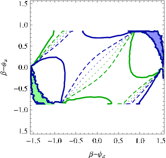
Figure 1: Contour plots of EdE_{d} for Λ=1019​GeV\Lambda=10^{19}{\rm~GeV}. The left figure corresponds to the analytic formula, eq. (25). Solid/dashed/dotted lines correspond to the absolute values of 1/0.3/0.1, blue lines correspond to negative values, green lines to positive ones. The right figure shows 2.5​Δd,23/Qd,232.5\Delta_{d,23}/Q_{d,23} where Δd,23\Delta_{d,23} has been obtained by numerically solving the RGEs. The rescaling was done in order to make the comparison to the analytical result easier.

In fig. 1 contours of EdE_{d} are plotted. The parameter range −π2<β−ψd,u<π2-\frac{\pi}{2}<\beta-\psi_{d,u}<\frac{\pi}{2} is sufficient as EdE_{d} is invariant under the shift β−ψd,u→β−ψd,u+π\beta-\psi_{d,u}\to\beta-\psi_{d,u}+\pi. As cut-off Λ=1019​GeV\Lambda=10^{19}{\rm~GeV} has been chosen as it is the scenario where maximal FCNCs can be expected and largest deviations of the leading log approximation. For this cut-off the grey shaded rectangles are not accessible as some Yukawa couplings become non-perturbative below Λ=1019​GeV\Lambda=10^{19}{\rm~GeV}. As will be shown in section 5 EdE_{d} can easily be 𝒪⁡(1)\mathcal{O}(1) while still satisfying the bounds on exotic contributions to the FCNCs.

To evaluate the accuracy of the analytical formulae we have calculated the flavour violating Higgs coupling Δd​ 23\Delta_{d\,23} solving numerically the full one-loop RGEs in the appendix.22 2 We have used β−ψe=0\beta-\psi_{e}=0 but the result is independent unless cos⁡(β−ψe)→0\cos(\beta-\psi_{e})\to 0. We show in fig. 1(b) Δd​ 23/Qd​ 23\Delta_{d\,23}/Q_{d\,23} and we find a very good agreement with the value EdE_{d} calculated analytically in eqs. (23) and (25) up to an overall factor of 2.5 (due to the large, flavour independent, effects in the running of the strong coupling constant and the top Yukawa coupling, which are not contemplated by the leading log approximation). We find, nevertheless, a new feature: There are regions with flipped sign at the top right and bottom left of the figure which are shown shaded. In these regions, differences in the running of Yd(1)Y_{d}^{(1)} compared to Yd(2)Y_{d}^{(2)}, not present in the leading log approximation, lead to a change of the sign of MdM_{d}, cf. eq. (10). Diagonalizing the quark masses, eqs. (15), this sign is transferred to Δd\Delta_{d}.

Before deriving upper bounds on the flavour off-diagonal couplings we will present our approximate formulae in two parameterizations widely used in the literature: the Wolfenstein parameterization of the CKM matrix and the Cheng & Sher parameterization of flavour violating couplings in a general 2HDM.

In the Wolfenstein parameterization

Using the Wolfenstein parameterization of the CKM matrix [4]:

VC​K​M=(1−λ22λA​λ3​(ρ−i​η)−λ1−λ22A​λ2A​λ3​(1−ρ−i​η)−A​λ21)+𝒪⁡(λ4)V_{CKM}=\left(\begin{array}[]{ccc}1-\frac{\lambda^{2}}{2}&\lambda&A\lambda^{3}(\rho-i\eta)\\ -\lambda&1-\frac{\lambda^{2}}{2}&A\lambda^{2}\\ A\lambda^{3}(1-\rho-i\eta)&-A\lambda^{2}&1\end{array}\right)+\mathcal{O}(\lambda^{4}) (26)

with λ≈0.2\lambda\approx 0.2, A≈0.8A\approx 0.8, ρ≈0.2\rho\approx 0.2 and η≈0.3\eta\approx 0.3 [5] and the approximate expressions

Mud​i​a​g.∼v2​diag​(λ6,λ3,1),Mdd​i​a​g.∼v2​diag​(λ6,λ4,λ2),M_{u}^{diag.}\sim\frac{v}{\sqrt{2}}{\rm diag}(\lambda^{6},\lambda^{3},1),\ \ \ M_{d}^{diag.}\sim\frac{v}{\sqrt{2}}{\rm diag}(\lambda^{6},\lambda^{4},\lambda^{2}), (27)

we get the following estimates:

[Qu]12\displaystyle[Q_{u}]_{12} ∼λ12,\displaystyle\sim\lambda^{12}, [Qu]13\displaystyle[Q_{u}]_{13} ∼λ8,\displaystyle\sim\lambda^{8}, [Qu]23\displaystyle[Q_{u}]_{23} ∼λ6,\displaystyle\sim\lambda^{6}, (28)
[Qd]12\displaystyle[Q_{d}]_{12} ∼λ9,\displaystyle\sim\lambda^{9}, [Qd]13\displaystyle[Q_{d}]_{13} ∼λ5,\displaystyle\sim\lambda^{5}, [Qd]23\displaystyle[Q_{d}]_{23} ∼λ4,\displaystyle\sim\lambda^{4}, (29)

and smaller values for the (21),(31),(32)(21),(31),(32) entries.

In the Cheng & Sher parameterization

The non-diagonal couplings of 2HDM are often parameterized as [6]:

(Δu)i​j=λi​ju​mu​i​mu​jv,(Δd)i​j=λi​jd​md​i​md​jv.(\Delta_{u})_{ij}=\lambda^{u}_{ij}\frac{\sqrt{m_{u\,i}m_{u\,j}}}{v},~~~~~~~~~(\Delta_{d})_{ij}=\lambda^{d}_{ij}\frac{\sqrt{m_{d\,i}m_{d\,j}}}{v}. (30)

Bounds on the coefficients λi​ju,d\lambda_{ij}^{u,d} have been derived from experimental results e.g. in [7]. These bounds depend on the masses of the Higgs bosons and on whether the parameters λi​ju,d\lambda_{ij}^{u,d} are assumed to be universal or to posses some kind of hierarchy. We do not assume universality. Instead the Yukawa alignment condition leads to:

|λ12u|\displaystyle|\lambda^{u}_{12}| ∼6×10⁻⁷​Eu,\displaystyle\sim 6\times 10^{-7}\ E_{u}, |λ13u|\displaystyle|\lambda^{u}_{13}| ∼10−4​Eu,\displaystyle\sim 10^{-4}\ E_{u}, |λ23u|\displaystyle|\lambda^{u}_{23}| ∼7×10⁻⁵​Eu,\displaystyle\sim 7\times 10^{-5}\ E_{u}, (31)
|λ12d|\displaystyle|\lambda^{d}_{12}| ∼5×10⁻⁴​Ed,\displaystyle\sim 5\times 10^{-4}\ E_{d}, |λ13d|\displaystyle|\lambda^{d}_{13}| ∼6×10⁻²​Ed,\displaystyle\sim 6\times 10^{-2}\ E_{d}, |λ23d|\displaystyle|\lambda^{d}_{23}| ∼0.1​Ed.\displaystyle\sim 0.1\ E_{d}. (32)

5 Experimental Bounds

In general, there are numerous experimental bounds on the parameters of 2HDMs. Constraints derived for the type I or type II apply also in our scenario as it is more general. In [2] bounds on the aligned 2HDM have been studied explicitly. As the alignment condition is broken by radiative corrections, in addition tree-level FCNCs are present. This leads to further constraints on the parameters of this type of 2HDMs, as FCNCs are known from experiment to be highly suppressed.

5.1 Meson-antimeson mixing

Stringent experimental bounds on FCNCs come from meson-antimeson mixing. In the SM this mixing can occur only at loop level while in a general 2HDM there is also a tree level mediation, see fig. 2(a). As the flavour eigenstates are thus not mass eigenstates this mixing leads to tiny mass differences that have been determined experimentally for Bd0,Bs0,D0B_{d}^{0},B_{s}^{0},D^{0} and K0K^{0} mesons. Here, we treat only the Bs0−B¯s0B_{s}^{0}-\bar{B}_{s}^{0} system as it gives the strongest constraints (see e.g. eqs. (31) and (32)). The effective Hamiltonian of the Δ​B=2\Delta B=2 transition Bs0↔B¯s0B_{s}^{0}\leftrightarrow\bar{B}^{0}_{s} is at scale ∼mZ\sim m_{Z}:

Heff.Δ​B=2=∑i,aCia​(mZ)​Qia​(mZ),H_{\rm eff.}^{\Delta B=2}=\sum_{i,a}C_{i}^{a}(m_{Z})Q_{i}^{a}(m_{Z}), (33)

where in a 2HDM with flavour violation at tree level the relevant operators are:

Q1S​L​L=(b¯R​sL)​(b¯R​sL),\displaystyle Q_{1}^{SLL}=(\bar{b}_{R}s_{L})(\bar{b}_{R}s_{L}), Q1S​R​R=(b¯L​sR)​(b¯L​sR),\displaystyle Q_{1}^{SRR}=(\bar{b}_{L}s_{R})(\bar{b}_{L}s_{R}), Q2L​R=(b¯R​sL)​(b¯L​sR).\displaystyle Q_{2}^{LR}=(\bar{b}_{R}s_{L})(\bar{b}_{L}s_{R}). (34)

The corresponding Wilson coefficients can be read off the effective Hamiltonian to be:

C1S​L​L\displaystyle C_{1}^{SLL} =−(Δd​ 23∗)22​(sα−β2mH2+cα−β2mh2−1mA2)\displaystyle=-\frac{(\Delta_{d\,23}^{*})^{2}}{2}\left(\frac{s^{2}_{\alpha\!-\!\beta}}{m_{H}^{2}}+\frac{c^{2}_{\alpha\!-\!\beta}}{m_{h}^{2}}-\frac{1}{m_{A}^{2}}\right) C1S​R​R\displaystyle C_{1}^{SRR} =−(Δd​ 32)22​(sα−β2mH2+cα−β2mh2−1mA2)\displaystyle=-\frac{(\Delta_{d\,32})^{2}}{2}\left(\frac{s^{2}_{\alpha\!-\!\beta}}{m_{H}^{2}}+\frac{c^{2}_{\alpha\!-\!\beta}}{m_{h}^{2}}-\frac{1}{m_{A}^{2}}\right) (35)
C2L​R\displaystyle C_{2}^{LR} =−Δd​ 23∗​Δd​ 32​(sα−β2mH2+cα−β2mh2+1mA2)\displaystyle=-\Delta_{d\,23}^{*}\Delta_{d\,32}\left(\frac{s^{2}_{\alpha\!-\!\beta}}{m_{H}^{2}}+\frac{c^{2}_{\alpha\!-\!\beta}}{m_{h}^{2}}+\frac{1}{m_{A}^{2}}\right) (36)

and the meson-antimeson mass difference can be calculated as:

Δ​mBs=|Δ​mBsSM+23​mBs​FBs2​[P2L​R​C2L​R​(mZ)+P1S​L​L​(C1S​L​L​(mZ)+C1S​R​R​(mZ))]|,\Delta m_{B_{s}}=\left|\Delta m_{B_{s}}^{\rm SM}+\frac{2}{3}m_{B_{s}}F_{B_{s}}^{2}\left[P_{2}^{LR}C_{2}^{LR}(m_{Z})+P_{1}^{SLL}\left(C_{1}^{SLL}(m_{Z})+C_{1}^{SRR}(m_{Z})\right)\right]\right|, (37)

where the coefficients PiaP_{i}^{a} include both the renormalization group evolution from the high scale mZm_{Z} down to low energy ∼mBs\sim m_{B_{s}} and the hadronization of the quarks to mesons. They can be calculated using the formulae in [8] and lattice QCD results from [9]. For the Bs0−B¯s0B^{0}_{s}-\bar{B}^{0}_{s}-system we get P2L​R=3.0P_{2}^{LR}=3.0 and P1S​L​L=−1.9P_{1}^{SLL}=-1.9. As [Δd]i​j≫[Δd]j​i[\Delta_{d}]_{ij}\gg[\Delta_{d}]_{ji} for j>ij>i the term involving C1S​R​RC_{1}^{SRR} is always neglible, whereas C2L​RC_{2}^{LR} dominates only for degenerate Higgs masses or in the decoupling limit (cα−β→0,mH≈mAc_{\alpha\!-\!\beta}\rightarrow 0,\ m_{H}\approx m_{A}). Therefore:

Δ​mBs\displaystyle\Delta m_{B_{s}} ≃\displaystyle\simeq |Δ​mBsSM+13​mBs​FBs2​P1S​L​L​Δd​ 23∗2​(sα−β2mH2+cα−β2mh2−1mA2)|,\displaystyle\left|\Delta m_{B_{s}}^{\rm SM}+\frac{1}{3}m_{B_{s}}F_{B_{s}}^{2}P_{1}^{SLL}\Delta_{d\,23}^{*2}\left(\frac{s^{2}_{\alpha\!-\!\beta}}{m_{H}^{2}}+\frac{c^{2}_{\alpha\!-\!\beta}}{m_{h}^{2}}-\frac{1}{m_{A}^{2}}\right)\right|, (38)
Δ​mBs\displaystyle\Delta m_{B_{s}} ≃\displaystyle\simeq |Δ​mBsSM+23​mBs​FBs2​P2L​R​Δd​ 23∗​Δd​ 32​(sα−β2mH2+cα−β2mh2+1mA2)|(degeneratemasses ordecoupling limit).\displaystyle\left|\Delta m_{B_{s}}^{\rm SM}+\frac{2}{3}m_{B_{s}}F_{B_{s}}^{2}P_{2}^{LR}\Delta_{d\,23}^{*}\Delta_{d\,32}\left(\frac{s^{2}_{\alpha\!-\!\beta}}{m_{H}^{2}}+\frac{c^{2}_{\alpha\!-\!\beta}}{m_{h}^{2}}+\frac{1}{m_{A}^{2}}\right)\right|\ \ \ \left(\begin{subarray}{c}\text{\footnotesize\mbox{degenerate}}\\ \text{\footnotesize\mbox{masses or}}\\ \text{\footnotesize\mbox{decoupling limit}}\end{subarray}\right). (39)

The SM prediction for the mass difference Δ​mBsSM=(135±20)⋅10−13\Delta m_{B_{s}}^{\rm SM}=(135\pm 20)\cdot 10^{-13} GeV [10] agrees quite well with the experimental value Δ​mBsexp.=(117.0±0.8)⋅10−13\Delta m_{B_{s}}^{\rm exp.}=(117.0\pm 0.8)\cdot 10^{-13} GeV [5]. Nevertheless there is room for new physics as long as the new contribution to the mass difference is smaller than the theoretical uncertainty, i.e. 20⋅10−1320\cdot 10^{-13} GeV. Using eq. (21) this leads to the approximate bound (we take FBs=238.8±9.5F_{B_{s}}=238.8\pm 9.5 MeV [9], mBs=5.37m_{B_{s}}=5.37 GeV [5] and values for the quark masses at mZm_{Z} from [11]):

|sα−β2mH2+cα−β2mh2−1mA2|​|Ed|2≲1(80​Gev)2.\left|\frac{s^{2}_{\alpha\!-\!\beta}}{m_{H}^{2}}+\frac{c^{2}_{\alpha\!-\!\beta}}{m_{h}^{2}}-\frac{1}{m_{A}^{2}}\right||E_{d}|^{2}\lesssim\frac{1}{(80\mathrm{~Gev})^{2}}. (40)

Thus, even for light Higgs masses, 𝒪⁡(100​GeV)\mathcal{O}(100\ \rm GeV), the present experimental constraints from meson-antimeson mixing allow EdE_{d} to be of 𝒪⁡(1)\mathcal{O}(1). In the case of degenerate masses or the decoupling limit the bound is even weaker:

|sα−β2mH2+cα−β2mh2+1mA2|​|Ed|2≲1(20​Gev)2.\left|\frac{s^{2}_{\alpha\!-\!\beta}}{m_{H}^{2}}+\frac{c^{2}_{\alpha\!-\!\beta}}{m_{h}^{2}}+\frac{1}{m_{A}^{2}}\right||E_{d}|^{2}\lesssim\frac{1}{(20\mathrm{~Gev})^{2}}. (41)
\fmfframe

(10,0)(0,5)


(a) Bs−B¯sB_{s}-\bar{B}_{s} mixing††feynman-diagram: (Feynman diagram, (x5)
\fmfframe

(10,)(0,5)


(b) B¯s→μ+​μ−\bar{B}_{s}\to\mu^{+}\mu^{-} ††feynman-diagram: (Feynman diagram, (x5)
Figure 2: Feynman diagrams for tree level flavour changing processes in a general 2HDM

5.2 Leptonic B decays

The decay B¯s→l+​l−​(l=e,μ,τ)\bar{B}_{s}\rightarrow l^{+}l^{-}\ (l=e,\mu,\tau), based on the flavour transition b→sb\rightarrow s, is another example of a process that can be mediated at tree level in a general 2HDM (see fig. 2(b)) but neither in the SM nor in an aligned 2HDM. As the branching ratio depends on the lepton Yukawa coupling one expects the decay B¯s→τ+​τ−\bar{B}_{s}\rightarrow\tau^{+}\tau^{-} to be favoured. However, the produced τ\tau’s decay immediately to jets and leptons whose observed invariant mass will not reconstruct back to the mass of the B meson, so that these decays cannot be tagged in detectors [12]. In contrast, tagging B¯s→μ+​μ−\bar{B}_{s}\rightarrow\mu^{+}\mu^{-} is rather easy leading to an unparalleled bound on the branching ratio. Integrating out the Higgs boson, the matrix element for the hh exchange is, assuming real Δe​ 22\Delta_{e\,22} (see Feynman rule (74)):

ℳB¯s→μ+​μ−h=14​cα−β​(Δd​ 23−Δd​ 32∗)​⟨B¯s|​s¯​γ5​b​|0⟩​1mh2​(−mμv​sα−β+cα−β​Δe​ 22)​μ¯​μ,\mathcal{M}_{\bar{B}_{s}\rightarrow\mu^{+}\mu^{-}}^{h}=\frac{1}{4}c_{\alpha-\beta}(\Delta_{d\,23}-\Delta_{d\,32}^{*})\bra{\bar{B}_{s}}\bar{s}\gamma^{5}b\ket{0}\frac{1}{m_{h}^{2}}\left(-\frac{m_{\mu}}{v}s_{\alpha-\beta}+c_{\alpha-\beta}\Delta_{e\,22}\right)\bar{\mu}\mu, (42)

since ⟨B¯s|​s¯​b​|0⟩\bra{\bar{B}_{s}}\bar{s}b\ket{0} is zero, as B¯s\bar{B}_{s} is parity-odd, whereas s¯​b\bar{s}b is parity-even (see e.g. [13]). On the other hand, the matrix element for HH exchange is of the same form as eq. (42), with the replacements cα−β→sα−β,sα−β→−cα−β,mh→mHc_{\alpha-\beta}\rightarrow s_{\alpha-\beta},\ s_{\alpha-\beta}\rightarrow-c_{\alpha-\beta},\ m_{h}\rightarrow m_{H}. Lastly, the invariant amplitude for the exchange of a pseudo-scalar AA can be inferred from eq. (75) to be:

ℳB¯s→μ+​μ−A=14​(Δd​ 23+Δd​ 32∗)​⟨B¯s|​s¯​γ5​b​|0⟩​1mA2​Δe​ 22​μ¯​γ5​μ.\mathcal{M}_{\bar{B}_{s}\rightarrow\mu^{+}\mu^{-}}^{A}=\frac{1}{4}(\Delta_{d\,23}+\Delta_{d\,32}^{*})\bra{\bar{B}_{s}}\bar{s}\gamma^{5}b\ket{0}\frac{1}{m_{A}^{2}}\Delta_{e\,22}\ \bar{\mu}\gamma^{5}\mu. (43)

The decay rate can now be straightforwardly calculated from the decay amplitudes. Using

⟨B¯s|​s¯​γ5​b​|0⟩≈i​fB​mBs,\bra{\bar{B}_{s}}\bar{s}\gamma^{5}b\ket{0}\approx if_{B}m_{B_{s}}, (44)

and neglecting again terms proportional to [Δd]j​i,j>i[\Delta_{d}]_{ji,j>i} we obtain:

ΓB¯s→μ+​μ−=fBs2​mBs364​π|Δd​ 23|2×{Δe​ 222mA4+|sα−βmH2​(mμv​cα−β+Δe​ 22​sα−β)+cα−βmh2​(−mμv​sα−β+Δe​ 22​cα−β)|2}.\Gamma_{\bar{B}_{s}\rightarrow\mu^{+}\mu^{-}}=\frac{f_{B_{s}}^{2}m_{B_{s}}^{3}}{64\pi}|\Delta_{d\,23}|^{2}\ \times\\ \left\{\frac{\Delta_{e\,22}^{2}}{m_{A}^{4}}+\left|\frac{s_{\alpha\!-\!\beta}}{m_{H}^{2}}\left(\frac{m_{\mu}}{v}c_{\alpha\!-\!\beta}+\Delta_{e\,22}s_{\alpha\!-\!\beta}\right)+\frac{c_{\alpha\!-\!\beta}}{m_{h}^{2}}\left(-\frac{m_{\mu}}{v}s_{\alpha\!-\!\beta}+\Delta_{e\,22}c_{\alpha\!-\!\beta}\right)\right|^{2}\right\}. (45)

Requiring that the tree level alone does not exceed the present experimental bound BR⁡(B¯s→μ+​μ−)<4.7⋅10−8{\rm BR}(\bar{B}_{s}\rightarrow\mu^{+}\mu^{-})<4.7\cdot 10^{-8} [5] we find for Δe​ 22≫mμv\Delta_{e\,22}\gg\frac{m_{\mu}}{v}:

1mA4+|sα−β2mH2+cα−β2mh2|2​Δe​ 22​|Ed|≲1(600​Gev)2.\sqrt{\frac{1}{m_{A}^{4}}+\left|\frac{s_{\alpha\!-\!\beta}^{2}}{m_{H}^{2}}+\frac{c_{\alpha\!-\!\beta}^{2}}{m_{h}^{2}}\right|^{2}}\Delta_{e\,22}|E_{d}|\lesssim\frac{1}{(600\mathrm{~Gev})^{2}}. (46)

Hence for Higgs masses of 𝒪⁡(100​GeV)\mathcal{O}(100\ \rm GeV) and EdE_{d} of 𝒪⁡(1)\mathcal{O}(1) there is only a conflict for tan⁡(ψe−β)∼Δe​ 22​vmμ≳50\tan(\psi_{e}-\beta)\sim\Delta_{e\,22}\frac{v}{m_{\mu}}\gtrsim 50. The opposite case, Δe​ 22≪mμv\Delta_{e\,22}\ll\frac{m_{\mu}}{v}, results in a bound on EdE_{d} and the Higgs masses only. However, for generic Higgs masses the bound coming from Bs−B¯sB_{s}-\bar{B}_{s} mixing is stronger.

6 Conclusions and outlook

We have studied in this letter the general two Higgs doublet model imposing that the Yukawa couplings for each fermion type are aligned at a high energy cut-off scale. This hypothesis guarantees the absence of new sources of flavour violation at tree level. We have shown, however, that quantum corrections spoil in general the alignment condition, inducing small flavour violating Higgs couplings at low energies. Without imposing ad hoc discrete symmetries and in the absence of tunings, the radiatively induced flavour violation in the Higgs sector yields the minimal size of the exotic contributions to the FCNCs in any 2HDM. We have shown that, for a wide range of parameters, this exotic contribution is well below the experimental constraints from meson-antimeson mixing and leptonic BB-decays.

In this letter we have concentrated on the constraints in the hadronic sector although the analysis can be extended to the leptonic sector. In the minimal extension of the Standard Model with one extra Higgs doublet, the Yukawa alignment in the leptonic sector is preserved after including the radiative corrections, due to the exactly preserved family lepton numbers. However, this scenario is incompatible with the observed neutrino oscillations. In a forthcoming publication [14] we will analyse the implications for the lepton flavour violating processes of the 2HDM with heavy right-handed neutrinos, necessary to generate neutrino masses through the see-saw mechanism.

Acknowledgements

We are grateful to Andrzej J. Buras, Gino Isidori and Tillmann Heidsieck for their valuable advice in the calculation of the experimental constraints on the 2HDM from B physics. This work was partially supported by the DFG cluster of excellence “Origin and Structure of the Universe” and by the Graduiertenkolleg “Particle Physics at the Energy Frontier of New Phenomena”.

Note added:

Simultaneously to the submission of this manuscript, the related works [15, 16] appeared. Our conclusions agree in the aspects where the analyses overlap.

Appendix A RGEs of the Yukawa couplings

The Renormalization Group Equation of the Yukawa couplings reads

16​π2​μ​d​Yfd​μ=βYf,16\pi^{2}\mu\frac{\mathrm{d}Y_{f}}{\mathrm{d}\mu}=\beta_{Y_{f}}, (47)

where

βYu(k)\displaystyle\beta_{Y_{u}^{(k)}} =\displaystyle= auYu(k)+∑l=1,2[3Tr(Yu(k)Yu(l)†+Yd(k)†Yd(l))+Tr(Ye(k)†Ye(l))]Yu(l)\displaystyle a_{u}Y_{u}^{(k)}+\sum_{l=1,2}\left[3\mathrm{Tr}\left(Y_{u}^{(k)}Y_{u}^{(l)\dagger}+Y_{d}^{(k)\dagger}Y_{d}^{(l)}\right)+\mathrm{Tr}\left(Y_{e}^{(k)\dagger}Y_{e}^{(l)}\right)\right]Y_{u}^{(l)} (48)
+∑l=1,2(−2Yd(l)Yd(k)†Yu(l)+Yu(k)Yu(l)†Yu(l)+12Yd(l)Yd(l)†Yu(k)+12Yu(l)Yu(l)†Yu(k)),\displaystyle+\sum_{l=1,2}\left(-2Y_{d}^{(l)}Y_{d}^{(k)\dagger}Y_{u}^{(l)}+Y_{u}^{(k)}Y_{u}^{(l)\dagger}Y_{u}^{(l)}+\frac{1}{2}Y_{d}^{(l)}Y_{d}^{(l)\dagger}Y_{u}^{(k)}+\frac{1}{2}Y_{u}^{(l)}Y_{u}^{(l)\dagger}Y_{u}^{(k)}\right),
βYd(k)\displaystyle\beta_{Y_{d}^{(k)}} =\displaystyle= adYd(k)+∑l=1,2[3Tr(Yu(k)†Yu(l)+Yd(k)Yd(l)†)+Tr(Ye(k)Ye(l)†)]Yd(l)\displaystyle a_{d}Y_{d}^{(k)}+\sum_{l=1,2}\left[3\mathrm{Tr}\left(Y_{u}^{(k)\dagger}Y_{u}^{(l)}+Y_{d}^{(k)}Y_{d}^{(l)\dagger}\right)+\mathrm{Tr}\left(Y_{e}^{(k)}Y_{e}^{(l)\dagger}\right)\right]Y_{d}^{(l)} (49)
+∑l=1,2(−2Yu(l)Yu(k)†Yd(l)+Yd(k)Yd(l)†Yd(l)+12Yu(l)Yu(l)†Yd(k)+12Yd(l)Yd(l)†Yd(k)),\displaystyle+\sum_{l=1,2}\left(-2Y_{u}^{(l)}Y_{u}^{(k)\dagger}Y_{d}^{(l)}+Y_{d}^{(k)}Y_{d}^{(l)\dagger}Y_{d}^{(l)}+\frac{1}{2}Y_{u}^{(l)}Y_{u}^{(l)\dagger}Y_{d}^{(k)}+\frac{1}{2}Y_{d}^{(l)}Y_{d}^{(l)\dagger}Y_{d}^{(k)}\right),
βYe(k)\displaystyle\beta_{Y_{e}^{(k)}} =\displaystyle= aeYe(k)+∑l=1,2[3Tr(Yu(k)†Yu(l)+Yd(k)Yd(l)†)+Tr(Ye(k)Ye(l)†)]Ye(l)\displaystyle a_{e}Y_{e}^{(k)}+\sum_{l=1,2}\left[3\mathrm{Tr}\left(Y_{u}^{(k)\dagger}Y_{u}^{(l)}+Y_{d}^{(k)}Y_{d}^{(l)\dagger}\right)+\mathrm{Tr}\left(Y_{e}^{(k)}Y_{e}^{(l)\dagger}\right)\right]Y_{e}^{(l)} (50)
+∑l=1,2(Ye(k)Ye(l)†Ye(l)+12Ye(l)Ye(l)†Ye(k)),\displaystyle+\sum_{l=1,2}\left(Y_{e}^{(k)}Y_{e}^{(l)\dagger}Y_{e}^{(l)}+\frac{1}{2}Y_{e}^{(l)}Y_{e}^{(l)\dagger}Y_{e}^{(k)}\right),

where afa_{f} (f=u,d,ef=u,d,e) stands for contributions due to gauge interactions, which are flavour-diagonal:

au\displaystyle a_{u} =−8​gs2−94​g2−1712​g′2,\displaystyle=-8g_{s}^{2}-\frac{9}{4}g^{2}-\frac{17}{12}g^{\prime 2}, (51)
ad\displaystyle a_{d} =−8​gs2−94​g2−512​g′2,\displaystyle=-8g_{s}^{2}-\frac{9}{4}g^{2}-\frac{5}{12}g^{\prime 2}, (52)
ae\displaystyle a_{e} =−94​g2−154​g′2,\displaystyle=-\frac{9}{4}g^{2}-\frac{15}{4}g^{\prime 2}, (53)

where gs,gg_{s},\ g and g′g^{\prime} are the gauge couplings constants of SU​(3)C,SU​(2)L{\rm SU}(3)_{C},\ {\rm SU}(2)_{L} and U​(1)Y{\rm U}(1)_{Y}, respectively. The terms in the first sum in the β\beta-function are due to the Higgs wave function renormalization, the first term in the second sum is due to the vertex renormalization (absent for leptons) and the last three (two) terms are due to the renormalization of the fermion wave function.

Appendix B Yukawa couplings at the EW scale

B.1 d-quarks

Yd(k)​(mZ)≈kd(k)​Yd+ϵd(k)​Yu​Yu†​Yd+δd(k)​Yd​Yd†​YdY_{d}^{(k)}(m_{Z})\approx k_{d}^{(k)}Y_{d}+\epsilon_{d}^{(k)}Y_{u}Y_{u}^{\dagger}Y_{d}+\delta_{d}^{(k)}Y_{d}Y_{d}^{\dagger}Y_{d} (54)

with

kd(1)\displaystyle k_{d}^{(1)} =cosψd+log⁡mZΛ16​π2[adcosψd+3cosψu∗cos(ψu−ψd)Tr(Yu†Yu)+3cosψdTr(YdYd†)+cosψecos(ψe∗−ψd)Tr(YeYe†)],\displaystyle=\cos\psi_{d}+\frac{\log\frac{m_{Z}}{\Lambda}}{16\pi^{2}}\Big[\begin{aligned} &a_{d}\cos\psi_{d}+3\cos\psi_{u}^{*}\cos(\psi_{u}-\psi_{d})\mathrm{Tr}(Y_{u}^{\dagger}Y_{u})\\ &+3\cos\psi_{d}\mathrm{Tr}(Y_{d}Y_{d}^{\dagger})+\cos\psi_{e}\cos(\psi_{e}^{*}-\psi_{d})\mathrm{Tr}(Y_{e}Y_{e}^{\dagger})\Big],\end{aligned} (55)
ϵd(1)\displaystyle\epsilon_{d}^{(1)} =log⁡mZΛ16​π2(12cosψd−2cosψu∗cos(ψu−ψd)),\displaystyle=\frac{\log\frac{m_{Z}}{\Lambda}}{16\pi^{2}}\left(\frac{1}{2}\cos\psi_{d}-2\cos\psi_{u}^{*}\cos(\psi_{u}-\psi_{d})\right), (56)
δd(1)\displaystyle\delta_{d}^{(1)} =3​log⁡mZΛ32​π2cosψd,\displaystyle=\frac{3\log\frac{m_{Z}}{\Lambda}}{32\pi^{2}}\cos\psi_{d}, (57)
kd(2)\displaystyle k_{d}^{(2)} =sinψd+log⁡mZΛ16​π2[adsinψd+3sinψu∗cos(ψu−ψd)Tr(Yu†Yu)+3sinψdTr(YdYd†)+sinψecos(ψe∗−ψd)Tr(YeYe†)],\displaystyle=\sin\psi_{d}+\frac{\log\frac{m_{Z}}{\Lambda}}{16\pi^{2}}\Big[\begin{aligned} &a_{d}\sin\psi_{d}+3\sin\psi_{u}^{*}\cos(\psi_{u}-\psi_{d})\mathrm{Tr}(Y_{u}^{\dagger}Y_{u})\\ &+3\sin\psi_{d}\mathrm{Tr}(Y_{d}Y_{d}^{\dagger})+\sin\psi_{e}\cos(\psi_{e}^{*}-\psi_{d})\mathrm{Tr}(Y_{e}Y_{e}^{\dagger})\Big],\end{aligned} (58)
ϵd(2)\displaystyle\epsilon_{d}^{(2)} =log⁡mZΛ16​π2(12sinψd−2sinψu∗cos(ψu−ψd)),\displaystyle=\frac{\log\frac{m_{Z}}{\Lambda}}{16\pi^{2}}\left(\frac{1}{2}\sin\psi_{d}-2\sin\psi_{u}^{*}\cos(\psi_{u}-\psi_{d})\right), (59)
δd(2)\displaystyle\delta_{d}^{(2)} =3​log⁡mZΛ32​π2sinψd;\displaystyle=\frac{3\log\frac{m_{Z}}{\Lambda}}{32\pi^{2}}\sin\psi_{d}; (60)

B.2 u-quarks

Yu(k)​(mZ)≈ku(k)​Yu+ϵu(k)​Yd​Yd†​Yu+δu(k)​Yu​Yu†​YuY_{u}^{(k)}(m_{Z})\approx k_{u}^{(k)}Y_{u}+\epsilon_{u}^{(k)}Y_{d}Y_{d}^{\dagger}Y_{u}+\delta_{u}^{(k)}Y_{u}Y_{u}^{\dagger}Y_{u} (61)

with

ku(1)\displaystyle k_{u}^{(1)} =cosψu+log⁡mZΛ16​π2[aucosψu+3cosψuTr(Yu†Yu)+3cosψd∗cos(ψd−ψu)Tr(YdYd†)+cosψe∗cos(ψe−ψu)Tr(YeYe†)],\displaystyle=\cos\psi_{u}+\frac{\log\frac{m_{Z}}{\Lambda}}{16\pi^{2}}\Big[\begin{aligned} &a_{u}\cos\psi_{u}+3\cos\psi_{u}\mathrm{Tr}(Y_{u}^{\dagger}Y_{u})+3\cos\psi_{d}^{*}\cos(\psi_{d}-\psi_{u})\mathrm{Tr}(Y_{d}Y_{d}^{\dagger})\\ &+\cos\psi_{e}^{*}\cos(\psi_{e}-\psi_{u})\mathrm{Tr}(Y_{e}Y_{e}^{\dagger})\Big],\end{aligned} (62)
ϵu(1)\displaystyle\epsilon_{u}^{(1)} =log⁡mZΛ16​π2(12cosψu−2cosψd∗cos(ψd−ψu)),\displaystyle=\frac{\log\frac{m_{Z}}{\Lambda}}{16\pi^{2}}\left(\frac{1}{2}\cos\psi_{u}-2\cos\psi_{d}^{*}\cos(\psi_{d}-\psi_{u})\right), (63)
δu(1)\displaystyle\delta_{u}^{(1)} =3​log⁡mZΛ32​π2cosψu,\displaystyle=\frac{3\log\frac{m_{Z}}{\Lambda}}{32\pi^{2}}\cos\psi_{u}, (64)
ku(2)\displaystyle k_{u}^{(2)} =sinψu+log⁡mZΛ16​π2[ausinψu+3sinψuTr(Yu†Yu)+3sinψd∗cos(ψd−ψu)Tr(YdYd†)+sinψe∗cos(ψe−ψu)Tr(YeYe†)],\displaystyle=\sin\psi_{u}+\frac{\log\frac{m_{Z}}{\Lambda}}{16\pi^{2}}\Big[\begin{aligned} &a_{u}\sin\psi_{u}+3\sin\psi_{u}\mathrm{Tr}(Y_{u}^{\dagger}Y_{u})+3\sin\psi_{d}^{*}\cos(\psi_{d}-\psi_{u})\mathrm{Tr}(Y_{d}Y_{d}^{\dagger})\\ &+\sin\psi_{e}^{*}\cos(\psi_{e}-\psi_{u})\mathrm{Tr}(Y_{e}Y_{e}^{\dagger})\Big],\end{aligned} (65)
ϵu(2)\displaystyle\epsilon_{u}^{(2)} =log⁡mZΛ16​π2(12sinψu−2sinψd∗cos(ψd−ψu)),\displaystyle=\frac{\log\frac{m_{Z}}{\Lambda}}{16\pi^{2}}\left(\frac{1}{2}\sin\psi_{u}-2\sin\psi_{d}^{*}\cos(\psi_{d}-\psi_{u})\right), (66)
δu(2)\displaystyle\delta_{u}^{(2)} =3​log⁡mZΛ32​π2sinψu;\displaystyle=\frac{3\log\frac{m_{Z}}{\Lambda}}{32\pi^{2}}\sin\psi_{u}; (67)

B.3 Leptons

As there are no vertex corrections in the leptonic sector, the coupling at the electroweak scale has a different structure:

Ye(k)​(mZ)≈ke(k)​Ye+δe(k)​Ye​Ye†​YeY_{e}^{(k)}(m_{Z})\approx k_{e}^{(k)}Y_{e}+\delta_{e}^{(k)}Y_{e}Y_{e}^{\dagger}Y_{e} (68)

with

ke(1)\displaystyle k_{e}^{(1)} =cosψe+log⁡mZΛ16​π2[aecosψe+3cosψu∗cos(ψu−ψe)Tr(Yu†Yu)+3cosψdcos(ψd∗−ψe)Tr(YdYd†)+cosψeTr(YeYe†)],\displaystyle=\cos\psi_{e}+\frac{\log\frac{m_{Z}}{\Lambda}}{16\pi^{2}}\Big[\begin{aligned} &a_{e}\cos\psi_{e}+3\cos\psi_{u}^{*}\cos(\psi_{u}-\psi_{e})\mathrm{Tr}(Y_{u}^{\dagger}Y_{u})\\ &+3\cos\psi_{d}\cos(\psi_{d}^{*}-\psi_{e})\mathrm{Tr}(Y_{d}Y_{d}^{\dagger})+\cos\psi_{e}\mathrm{Tr}(Y_{e}Y_{e}^{\dagger})\Big],\end{aligned} (69)
δe(1)\displaystyle\delta_{e}^{(1)} =3​log⁡mZΛ32​π2cosψe,\displaystyle=\frac{3\log\frac{m_{Z}}{\Lambda}}{32\pi^{2}}\cos\psi_{e}, (70)
ke(2)\displaystyle k_{e}^{(2)} =sinψe+log⁡mZΛ16​π2[aesinψe+3sinψu∗cos(ψu−ψe)Tr(Yu†Yu)+3sinψdcos(ψd∗−ψe)Tr(YdYd†)+sinψeTr(YeYe†)],\displaystyle=\sin\psi_{e}+\frac{\log\frac{m_{Z}}{\Lambda}}{16\pi^{2}}\Big[\begin{aligned} &a_{e}\sin\psi_{e}+3\sin\psi_{u}^{*}\cos(\psi_{u}-\psi_{e})\mathrm{Tr}(Y_{u}^{\dagger}Y_{u})\\ &+3\sin\psi_{d}\cos(\psi_{d}^{*}-\psi_{e})\mathrm{Tr}(Y_{d}Y_{d}^{\dagger})+\sin\psi_{e}\mathrm{Tr}(Y_{e}Y_{e}^{\dagger})\Big],\end{aligned} (71)
δe(2)\displaystyle\delta_{e}^{(2)} =3​log⁡mZΛ32​π2sinψe;\displaystyle=\frac{3\log\frac{m_{Z}}{\Lambda}}{32\pi^{2}}\sin\psi_{e}; (72)

Appendix C Feynman rules

\fmfframe

(3,3)(3,3)

††feynman-diagram: (Feynman diagram, (x2)
=−i2​[2​cα−β​mf​iv​δi​j+sα−β​((Δf+Δf†)i​j+(Δf−Δf†)i​j​γ5)]\displaystyle=-\frac{i}{2}\left[2c_{\alpha-\beta}\frac{m_{f\,i}}{v}\delta_{ij}+s_{\alpha-\beta}\left((\Delta_{f}+\Delta_{f}^{\dagger})_{ij}+(\Delta_{f}-\Delta_{f}^{\dagger})_{ij}\gamma^{5}\right)\right] (73)

for f=u,d,ef=u,d,e

\fmfframe

(3,3)(3,3)

††feynman-diagram: (Feynman diagram, (x2)
=−i2​[−2​sα−β​mf​iv​δi​j+cα−β​((Δf+Δf†)i​j+(Δf−Δf†)i​j​γ5)]\displaystyle=-\frac{i}{2}\left[-2s_{\alpha-\beta}\frac{m_{f\,i}}{v}\delta_{ij}+c_{\alpha-\beta}\left((\Delta_{f}+\Delta_{f}^{\dagger})_{ij}+(\Delta_{f}-\Delta_{f}^{\dagger})_{ij}\gamma^{5}\right)\right] (74)

for f=u,d,ef=u,d,e

\fmfframe

(3,3)(3,3)

††feynman-diagram: (Feynman diagram, (x2)
=12​[(Δf−Δf†)i​j+(Δf+Δf†)i​j​γ5]\displaystyle=\frac{1}{2}\left[(\Delta_{f}-\Delta_{f}^{\dagger})_{ij}+(\Delta_{f}+\Delta_{f}^{\dagger})_{ij}\gamma^{5}\right] (75)

for f=d,ef=d,e and for f=uf=u the same with negative sign

\fmfframe

(3,3)(3,3)

††feynman-diagram: (Feynman diagram, (x2)
=−i2​[(−Δu†​VC​K​M+VC​K​M​Δd)i​j+(Δu†​VC​K​M+VC​K​M​Δd)i​j​γ5]\displaystyle=-\frac{i}{\sqrt{2}}\left[(-\Delta_{u}^{\dagger}V_{CKM}+V_{CKM}\Delta_{d})_{ij}+(\Delta_{u}^{\dagger}V_{CKM}+V_{CKM}\Delta_{d})_{ij}\gamma^{5}\right] (76)

for quarks and VC​K​M​Δd→ΔeV_{CKM}\Delta_{d}\to\Delta_{e}, Δu→0\Delta_{u}\to 0 for leptons

Here mf​im_{f\,i} is the corresponding fermion mass and Δf\Delta_{f} is defined by eqs. (17), (18) and analogously for the leptons.

References