Keywords: Phase transitions into absorbing states (Theory), Population dynamics (Theory), Stochastic processes, Coarsening processes (Theory)
Three-fold way to extinction in populations of cyclically competing species
Abstract
Species extinction occurs regularly and unavoidably in ecological systems. The time scales for extinction can broadly vary and inform on the ecosystem’s stability. We study the spatio-temporal extinction dynamics of a paradigmatic population model where three species exhibit cyclic competition. The cyclic dynamics reflects the non-equilibrium nature of the species interactions. While previous work focusses on the coarsening process as a mechanism that drives the system to extinction, we found that unexpectedly the dynamics to extinction is much richer. We observed three different types of dynamics. In addition to coarsening, in the evolutionary relevant limit of large times, oscillating traveling waves and heteroclinic orbits play a dominant role. The weight of the different processes depends on the degree of mixing and the system size. By analytical arguments and extensive numerical simulations we provide the full characteristics of scenarios leading to extinction in one of the most surprising models of ecology.
pacs
87.23.Cc, 05.40.-a, 02.50.Ey1 Introduction
Stochastic many-particle systems provide a testing ground for non-equilibrium dynamics. In nature, systems frequently evolve away from equilibrium and then relax to an equilibrium steady state. Understanding the relaxation process is a central topic in non-equilibrium physics. Near-equilibrium fluctuations are governed by the same laws that hold in steady state and the transient is typically an exponential decay. Many systems, however, comprise absorbing states, which can be reached but never be left by the dynamics. In this case no fluctuations are present in the steady states. Such systems arise in a broad variety of problems, e.g. physics, chemistry or epidemics [1]. Much effort has been spent on the investigation of simple, diffusion-limited chemical reactions where the decay to equilibrium can obey power laws [2].
Understanding transitions into absorbing states is not only fundamental for non-equilibrium physics, but is also highly relevant for ecology. Here, absorbing states correspond to the extinction of species. Another characteristic feature of ecological systems are cyclic interactions. As a classic example, the work of Lotka and Volterra describes the dynamics of fish populations in the adriatic as persistent oscillations due to predator-prey interactions. Other examples include coral reef invertebrates [3], rodents in the high arctic tundra in Greenland [4], cyclic competition between different mating strategies of lizards [5] and chemical warfare of Escherichia coli bacteria under laboratory conditions [6].
Recent work has investigated cyclic competition in one-dimensional systems with no or only weak diffusion of the reacting agents [7, 8, 9, 10]. Coarse-graining of temporally growing and annihilating domains has been identified as the mechanism that eventually leads to species extinction. However, individual’s mobility may be significant and alter this picture qualitatively.
In this article, we investigate the spatio-temporal dynamics of extinction in a paradigmatic model of three species in cyclic competition. Individuals are positioned on a one-dimensional lattice and are equipped with fast mobility that leads to effective diffusion. The system possesses absorbing states in the form of extinction of two of the three species and, because of fluctuations, the dynamics eventually comes to rest there. However, the time-scales until extinction occurs provide information on the stability of species diversity [11]. We identify three distinct types of dynamics that lead to extinction. These types of dynamics arise from the possible influences that intrinsic fluctuations can have on the coarsening process and on the traveling waves that the cyclic dynamics induces. The different dynamics lead to characteristic dependences of the extinction-time probability on the elapsed time and the system size . We provide semi-phenomenological arguments that quantify the functional form and the scaling behaviour of the extinction-time probability. These arguments yield information on the emergence and characteristics of the different types of dynamics.
2 The model
Consider a stochastic, spatial variant of the May-Leonard model which serves as a prototype for cyclic, rock-paper-scissors-like species interactions. Three species compete with each other in a cyclic manner, at rate , and reproduce at rate upon availability of empty space :
| (1) | |||||
| (2) |
For increasingly large populations intrinsic fluctuations eventually become negligible. If in addition spatial structure is absent, i.e., if every individual can interact with every other in the population at equal probability, the population dynamics is aptly described by deterministic rate equations for the densities of the species and :
| (3) |
Hereby the indices are understood as modulo and denotes the total density. May and Leonard showed that these equations possess absorbing fixed points, corresponding to the survival of one of the species and to an empty system [12]. Furthermore a reactive fixed point exists that represents coexistence of all three species. Linear stability analysis shows that is unstable. The absorbing steady states that correspond to extinction, , and , are heteroclinic points. The Lyapunov function demonstrates that the trajectories of the deterministic equations (3), when initially close to the reactive fixed point, spiral outward on an invariant manifold. On this manifold the trajectories then approach the boundary of the phase space and form heteroclinic cycles, converging to the boundary and the absorbing states without ever reaching them.
However, intrinsic noise from finite-system sizes [13, 14] and spatial correlations alter the above behaviour [15, 16, 17, 18]. While fluctuations ultimately drive the system into one of the absorbing fixed points [19], the formation of spatial patterns can substantially delay extinction and promote species coexistence [16, 20, 21]. The resulting spatio-temporal dynamics of extinction is nontrivial and highly interesting.
3 Numerical results
We consider a one-dimensional lattice of sites with periodic boundary conditions. Each lattice site hosts a fixed number of individuals and empty spaces , such that the concentrations in the rate equations (3) are given by the number of particles of a specified type divided by . may hence be viewed as the carrying capacity of a lattice site. The reactions (2) occur between individuals on the same lattice site. Individuals may change place with another individual or an empty space on a neighbouring lattice site at rate . In order to keep the length scale, i.e. characteristic length scale for diffusion, fixed when changing the lattice spacing we have to rescale appropriately. In the continuum limit, where (3) holds, the exchange processes therefore lead to an effective diffusion of individuals at a diffusion constant and thus to coupling between the lattice sites. In our simulations we implemented a continuous-time Markov process with sequential updating. At each simulation step an individual is randomly chosen. It then either reacts with a randomly chosen individual of the same site or changes place with a randomly chosen individual of the two neighbouring stacks, at probabilities corresponding to the rates , and .
The population model introduced above possesses a net system size of which plays the role of an overall carrying capacity. For large enough and the intrinsic fluctuations have a strength proportional to the inverse square-root of [22]. Different equivalent ways therefore exist for performing the thermodynamic limit, e.g., increasing the number of individuals per lattice site, while keeping the lattice size fixed or increasing the lattice size , keeping fixed. Because for large a huge amount of exchange processes takes place between the reactions, requiring long computation time, we performed the thermodynamic limit in and kept fixed. The insensitivity of the results to the choice of the limit is supported by recent studies [10]. was chosen sufficiently large, such that was much smaller than the correlation length.
We here consider the case of equal reproduction and selection rates . Similar behaviour can be expected for , when is rescaled appropriately [20], and species dependent interaction rates [10, 23]. We chose a random initial configuration in which the density of the species approximately equals the ones of the internal fixed point of the rate equations (3).


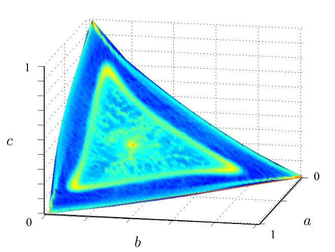
Our simulations reveal three distinct classes of dynamics (Figure 1). First, at short time scales stochastic effects lead to the emergence of domains due to coarsening. In this scenario, after a short coarsening process, domains emerge, whose order does not correspond to the rules of cyclic dominance, leading to oppositely moving fronts and hence immediate annihilation. Extinction occurs rapidly in this scenario. The coarsening dynamics to extinction has been extensively studied [7, 8, 9]. However, our simulations reveal a much richer dynamics to extinction. Two more processes dominate the dynamics for large times. Second, we observe situations where the population is almost entirely taken over by a species in cost of a second species, which dies out. A few individuals of the other surviving species are present in the system and, being the dominant one, slowly fixate. This scenario is intimately related to the heteroclinic orbits of the rate equations (3). The global dynamics moves along the boundary of the invariant manifold of (3). Spatial patterns are of minor importance. Third, the system can enter a state of propagating waves of cyclically aligned, uniform domains. These states are only metastable: fluctuating front positions result in domain-annihilation and eventual extinction. For small this effect was also denoted in [10] and corresponds to the spiral waves found in the two-dimensional model [20]. Rare events at the leading edge of the fronts cause the tunneling of domains and oscillating overall species densities.
Figure 2 provides a concrete picture of the different dynamical processes. The system’s state probability is projected onto the invariant manifold of the rate equations (3). The colour signifies the logarithmic probability to find a given net density of species on the manifold before reaching an absorbing fixed point. We recognize that the system spends considerable time in the vicinity of the boundary, especially near the corners of the simplex, corresponding to the heteroclinic orbits occurring in the second scenario. The stochastic limit cycle around the unstable fixed point reflects the oscillating traveling waves from the third scenario (see also, e.g., [25]). In the center single trajectories of non-oscillating waves are visible.
The influence of mobility is visualised in Figure 2. The Lyapunov function characterizes the system’s behavior: it is zero at the boundaries and increases monotonically to the unstable fixed point . therefore provides a measure for the distance of the system’s state from the boundaries. The logarithmic probability to find the system at a certain value of , depending on the diffusivity , is given in Figure 2. A drastic change in the system’s behavior occurs at a critical mobility . Above we observe only heteroclinic orbits, characterized by a high probability to find the system at small values of . For very small the system exhibits traveling waves, performing random walks in concentration space. Below both types of dynamics are present. The high probabilities for small values of indicate heteroclinic orbits, while the ridge at larger values is caused by oscillating traveling waves.

Quantification of the three different dynamical scenarios is feasible through the extinction-time probability, , meaning the probability density that two species go extinct at a certain time . Mathematically it gives the probability distribution function of first-passage times into one of the absorbing fixed points. In our simulations we varied from 1 to 2800 and set , i.e. in the region, where all types of dynamics arise simultaneously. Figure 3 shows the extinction-time probability distribution for various system sizes. The sharp peak at small times results from the annihilation of oppositely propagating waves as a result of the coarsening process, i.e. the first scenario. The functional form of the extinction-time probability distribution for intermediate and large times is determined by the heteroclinic orbits and propagating waves, the second and third types of dynamics. We find an exponentially decaying tail that is, for large , preceded by a intermediate asymptotic power-law interval. The length of this intermediate interval scales linearly with . The plateau or second maximum originates in the short term dynamics of the latter two scenarios.
4 Semi-phenomenological arguments
The characteristics of the critical behavior shown in Figure 2 can be understood through the spatial variant of the rate equations, (3). Following Ref. [26] the system’s dynamics on the invariant manifold can, through a nonlinear transformation to variables and , be recast in terms of the complex Ginzburg-Landau equation
| (4) |
with , , and [27]. The theory of front propagation into unstable states predicts that (4) always admits traveling waves as stable solutions [28]. Following a classic treatment of the problem of front-speed selection we obtain their wavelength as . At the critical diffusivity the wavelength exceeds the system size such that the fronts become unstable. From the condition and accounting for the rescaling factor mentioned in [27] we obtain , which is in very good agreement with our numerical results.
The behaviour of the extinction-time probability distribution can be understood through semi-phenomenological models. In the following we show how such models yield the shape of the extinction-time probability distribution and its dependence on . In particular, we give an explanation for the scaling behaviour of the power-law interval and the long-time exponential decay. We show that, depending on the system size, either heteroclinic orbits or traveling waves dominate the long-time dynamics.
The dynamics of the heteroclinic orbits can be quantified as follows. Consider a small density of individuals of species in a large pool of species []. Due to reproduction of empty space is as sparse as individuals are: . Simulations inform us that spatial patterns are not relevant in this scenario. We therefore consider a well-mixed system of size . Three reactions lead to the take-over of the population through the dominating species :
| at rate | ||||
| at rate | ||||
| at rate |
Here the rates are meant as transitions per unit time. The fast processes are in equilibrium and can be adiabatically eliminated for large , yielding . Species occurs at the same density as empty sites times . A series of reproduction events remains, each with an exponentially distributed waiting time. In the language of stochastic processes this is a pure birth process, studied arising in preferential attachment problems. The extinction-time probability distribution is thus given by a convolution over exponential functions. By applying the Laplace transform one can show that it can be expressed in closed form as
| (5) |
with rates [29]. One finally has to marginalize over the probability of starting with an initial density of species to obtain the extinction-time probability distribution as results from the heteroclinic-orbit dynamics:
| (6) |
For any reasonable the asymptotic behaviour is dominated by the term for the lowest initial concentration and the lowest reproduction rate : We thus find a -dependence of the exponential tail on the system size. For intermediate times we have to take the full convolution and marginalization sums of eq. (6) into account. Numerical evaluation indeed yields a power-law interval for uniformly distributed . The time of crossover between the power-law and the exponential decay scales with . We therefore find that the second type of dynamics, heteroclinic orbits, lead to the intermediate power-law regime in the extinction-time probability distribution. The exponential tail of this distribution can either result from heteroclinic orbits or from propagating waves as shown below.
The third type of spatio-temporal dynamics, propagating waves, is metastable. They disappear only through the rare annihilation of neighbouring fronts. By symmetry, the waves move with the same average velocity. For small the domain interfaces are sharp and therefore interact only on distances that are much smaller than the average domain size. The extinction dynamics in this scenario can therefore be described within an interface picture, where, in a comoving frame, the wave fronts behave as random walkers on a one dimensional lattice with diffusion coefficient . For larger long-range interactions between the interfaces become important, leading to a tunneling of domains. However, within the interface picture this merely corresponds to a relabeling of interfaces and therefore does not influence the extinction dynamics. Numerical simulations validate the assumption of normal diffusion. For a single series of subsequent domains the survival probability , meaning the probability that all three domains still coexist at time , follows as the survival probability of a single random walker between absorbing boundaries at distance . The probability distribution for the random walker to be at position and time when starting at obeys a diffusion equation subject to absorbing boundary conditions. The solution is well known:
| (7) |
with the coefficients being determined by the initial condition , see e.g. [30]. Averaging over space, the initial positions and identically distributed interval lengths yields the survival probability from the traveling-wave dynamics:
| (8) |
In the asymptotic limit the expression evaluates to . The extinction-time probability distribution follows as . What is the diffusion constant of the domain front? Brunet et al. proposed [31] that the diffusion constant for a broad class of stochastic propagating waves depends on as . Therewith the exponential decay of the extinction-time probability distribution’s tail, as resulting from the traveling-wave dynamics, is proportional to . This result is validated by our numerical simulations, see Figure 3 bottom right. Heteroclinic orbits and traveling waves both contribute to the asymptotic limit of the net extinction-time probability distribution : . Both contributions yield exponential decays at large times, but with different scalings in . For small systems the term in , resulting from the traveling-wave dynamics, dominates. In contrast, the -decay in resulting from heteroclinic orbits yields the major contribution when is large. In agreement with these analytical results we indeed find numerically that the exponential decay scales as for small and as for large (Figure 3). Numerically we identified the crossover between both regimes to occur at .
5 Conclusion
We investigated the spatio-temporal extinction dynamics in a three species stochastic population model with cyclic interactions. While previous work has mainly focused on the coarse graining process that drives the system to extinction we identified two more types of dynamics that are rare but due to their lifetime most important from an evolutionary perspective. The three classes of dynamics, namely rapid annihilation of domains, heteroclinic orbits, and traveling waves are correlated with features of the phase portrait and leave their fingerprints in the extinction-time probability distribution. The weight of these processes depends on the degree of mixing as well as on the system size. Based on the different dynamical scenarios we provided semi-phenomenological calculations that yield the functional form of this probability distribution and its dependence on the system size. We believe that our results are of general relevance as we expect a similar phenomenology in other systems described by the complex Ginzburg-Landau equation.
References
References
- [1] Hinrichsen H 2000 Adv. Phys. 49 815–958
- [2] Täuber U C, Howard M and Vollmayr-Lee B P 2005 J. Phys. A-Math. Gen. 38 R79–R131
- [3] Jackson J B C and Buss L 1975 Proc. Nat. Acad. Sci. USA 72 5160–5163
- [4] Gilg O, Hanski I and Sittler B 2001 Science 302 866–868
- [5] Sinervo B and Lively C M 1996 Nature 380 240–243
- [6] Kerr B, Riley M A, Feldman M W and Bohannan B J M 2002 Nature 418 171–174
- [7] Tainaka K 1988 J. Phys. Soc. Jpn. 57 2588–2590
- [8] Frachebourg L, Krapivsky P L and BenNaim E 1996 Phys. Rev. Lett. 77 2125–2128
- [9] Frachebourg L, Krapivsky P L and Ben-Naim E 1996 Phys. Rev. E 54 6186–6200
- [10] He Q, Mobilia M and Täuber U 2010 Phys. Rev. E 82
- [11] Cremer J, Reichenbach T and Frey E 2009 New J. Phys. 11 093029
- [12] May R and Leonard W 1975 SIAM J. Appl. Math. 29 243–253
- [13] Claussen J C and Traulsen A 2008 Phys. Rev. Lett. 100 058104
- [14] Boland R P, Galla T and McKane A J 2009 Phys. Rev. E 79 051131
- [15] Durrett R and Levin S 1998 Theor. Pop. Biol.
- [16] Szabó G and Fath G 2007 Phys. Rep. 446 97–216
- [17] Abta R, Schiffer M and Shnerb N M 2007 Phys. Rev. Lett. 98 098104
- [18] Peltomäki M and Alava M 2008 Phys. Rev. E 78 031906
- [19] Parker M and Kamenev A 2009 Phys. Rev. E 80 021129
- [20] Reichenbach T, Mobilia M and Frey E 2007 Nature 448 1046–1049
- [21] Efimov A, Shabunin A and Provata A 2008 Phys. Rev. E 78 056201
- [22] Gardiner C 2004 Handbook of Stochastic Methods (Springer-Verlag)
- [23] Venkat S and Pleimling M 2010 Phys. Rev. E 81 021917
- [24] Reichenbach T, Mobilia M and Frey E 2006 Phys. Rev. E 74 051907
- [25] Bladon A J, Galla T and McKane A J 2010 Phys. Rev. E 81 066122
- [26] Reichenbach T, Mobilia M and Frey E 2008 J. Theor. Biol. 254 368–383
- [27] Reichenbach T, Mobilia M and Frey E 2007 Phys. Rev. Lett. 99
- [28] van Saarlos W 2003 Phys. Rep. 386 29–222
- [29] Kannan D 1979 Introduction to stochastic processes (Elsevier North Holland)
- [30] Redner S 2001 A guide to first passage processes (Cambridge University Press)
- [31] Brunet E, Derrida B, Mueller A H and Munier S 2006 Phys. Rev. E 73 056126