跳到论文正文
W Papers独立论文阅读器 arXiv:1005.5697 论文正文 计算阅读时间 · 0%
引用这篇论文根据当前论文元数据生成,正式投稿前建议核对。


License: arXiv.org perpetual non-exclusive license
arXiv:1005.5697v1 [math.ST] 31 May 2010

Unbiased Estimation of a Sparse Vector in
White Gaussian Noise

Alexander Jung Affiliation: Institute of Communications and Radio-Frequency Engineering, Vienna University of TechnologyGusshausstrasse 25/389, 1040 Vienna, AustriaPhone: +43 1 58801 38963, Fax: +43 1 58801 38999, E-mail: {ajung, fhlawats}@nt.tuwien.ac.at    Zvika Ben-Haim Affiliation: Technion—Israel Institute of TechnologyHaifa 32000, Israel; e-mail: {zvikabh@tx, yonina@ee}.technion.ac.il    Franz Hlawatsch Affiliation: Institute of Communications and Radio-Frequency Engineering, Vienna University of TechnologyGusshausstrasse 25/389, 1040 Vienna, AustriaPhone: +43 1 58801 38963, Fax: +43 1 58801 38999, E-mail: {ajung, fhlawats}@nt.tuwien.ac.at       Yonina C. Eldar ††thanks: This work was supported by the FWF under Grant S10603-N13 (Statistical Inference) within the National Research Network SISE, by the WWTF under Grant MA 07-004 (SPORTS), by the Israel Science Foundation under Grant 1081/07, and by the European Commission under the FP7 Network of Excellence in Wireless Communications NEWCOM++ (contract no. 216715). Parts of this work were previously presented at ICASSP 2010, Dallas, TX, March 2010. Affiliation: Technion—Israel Institute of TechnologyHaifa 32000, Israel; e-mail: {zvikabh@tx, yonina@ee}.technion.ac.il
Abstract

We consider unbiased estimation of a sparse nonrandom vector corrupted by additive white Gaussian noise. We show that while there are infinitely many unbiased estimators for this problem, none of them has uniformly minimum variance. Therefore, we focus on locally minimum variance unbiased (LMVU) estimators. We derive simple closed-form lower and upper bounds on the variance of LMVU estimators or, equivalently, on the Barankin bound (BB). Our bounds allow an estimation of the threshold region separating the low-SNR and high-SNR regimes, and they indicate the asymptotic behavior of the BB at high SNR. We also develop numerical lower and upper bounds which are tighter than the closed-form bounds and thus characterize the BB more accurately. Numerical studies compare our characterization of the BB with established biased estimation schemes, and demonstrate that while unbiased estimators perform poorly at low SNR, they may perform better than biased estimators at high SNR. An interesting conclusion of our analysis is that the high-SNR behavior of the BB depends solely on the value of the smallest nonzero component of the sparse vector, and that this type of dependence is also exhibited by the performance of certain practical estimators.

Index Terms: 
Sparsity, unbiased estimation, denoising, Cramér–Rao bound, Barankin bound, Hammersley–Chapman–Robbins bound, locally minimum variance unbiased estimator.

I Introduction

Research in the past few years has led to a recognition that the performance of signal processing algorithms can be boosted by exploiting the tendency of many signals to have sparse representations. Applications of this principle include signal reconstruction (e.g. in the context of compressed sensing [1, 2]) and signal enhancement (e.g. in the context of image denoising and deblurring [3, 4, 5]).

In this work, we consider the estimation of an SS-sparse, finite-dimensional vector 𝐱∈ℝN\mathbf{x}\!\in\!\mathbb{R}^{N}\!. By “SS-sparse” we mean that the vector 𝐱\mathbf{x} has at most SS nonzero entries, which is denoted by ‖𝐱‖0≜|supp⁡(𝐱)|≤S{\|\mathbf{x}\|}_{0}\triangleq|\supp(\mathbf{x})|\leq S, where supp⁡(𝐱)\supp(\mathbf{x}) denotes the set of indices of the nonzero entries of 𝐱\mathbf{x}. The “sparsity” SS is assumed to be known, and typically S≪NS\!\ll\!N. However, the positions of the nonzero entries (i.e., supp⁡(𝐱)\supp(\mathbf{x})) as well as the values of the nonzero entries are unknown. We investigate how much we can gain in estimation accuracy by knowing a priori that the vector 𝐱\mathbf{x} is SS-sparse. We will use the frequentist setting [6] of estimation theory, i.e., we will model 𝐱\mathbf{x} as unknown but deterministic. This is in contrast to Bayesian estimation theory, where one treats 𝐱\mathbf{x} as a random vector whose probability density function (pdf) or certain moments thereof are assumed to be known. In the Bayesian setting, the sparsity can be modeled by using a pdf that favors sparse vectors, see e.g. [7, 8, 9].

A fundamental concept in the frequentist setting is that of unbiasedness [6, 10, 11]. An unbiased estimator is one whose expectation always equals the true underlying vector 𝐱{\bf x}. The restriction to unbiased estimators is important as it excludes trivial and practically useless estimators, and it allows us to study the difficulty of the estimation problem using established techniques such as the Cramér–Rao bound (CRB) [12, 10, 11]. Another justification of unbiasedness is that for typical estimation problems, when the variance of the noise is low, it is necessary for an estimator to be unbiased in order to achieve a small mean-squared estimation error (MSE) [6].

These reasons notwithstanding, there is no guarantee that unbiased estimators are necessarily optimal. In fact, in many settings, including the scenario described in this paper, there exist biased estimators which are strictly better than any unbiased technique in terms of MSE [13, 14, 15]. Nevertheless, for simplicity and because of the reasons stated above, we focus on bounds for unbiased estimation in this work. As we will see, bounds on unbiased techniques give some indication of the general difficulty of the setting, and as such some of our conclusions will be shown empirically to characterize biased techniques as well.

Our main contribution is a characterization of the optimal performance of unbiased estimators 𝐱^​(𝐲)\hat{\mathbf{x}}(\mathbf{y}) that are based on

observing

𝐲=𝐀𝐱+𝐧\mathbf{y}\hskip 0.56905pt=\hskip 0.56905pt\mathbf{A}\mathbf{x}+\mathbf{n} (1)

where 𝐀∈ℝM×N\mathbf{A}\!\in\!\mathbb{R}^{M\times N} (M≥NM\!\geq\!N) is a known matrix with orthonormal columns, i.e., 𝐀T​𝐀=𝐈N\mathbf{A}^{T}\hskip-0.56905pt\mathbf{A}=\mathbf{I}_{N}, and 𝐧∼𝒩⁡(𝟎,σ2​𝐈M)\mathbf{n}\sim\mathcal{N}(\mathbf{0},\sigma^{2}\mathbf{I}_{M}) denotes zero-mean white Gaussian noise with known variance σ2\sigma^{2} (here, 𝐈N\mathbf{I}_{N} denotes the identity matrix of size N×NN\times N). Note that without loss of generality we can then assume that 𝐀=Ê​𝐈N\mathbf{A}=Ê\mathbf{I}_{N} and M=NM=N, i.e., 𝐲=𝐱+𝐧\mathbf{y}=\mathbf{x}+\mathbf{n}, since premultiplication of the model (1) by 𝐀T\mathbf{A}^{T} will reduce the estimation problem to an equivalent problem 𝐲′=𝐀′​𝐱+𝐧′\mathbf{y}^{\prime}=\mathbf{A}^{\prime}\mathbf{x}+\mathbf{n}^{\prime} in which 𝐀′=𝐀T​𝐀=𝐈N\mathbf{A}^{\prime}=\mathbf{A}^{T}\hskip-0.56905pt\mathbf{A}=\mathbf{I}_{N} and the noise 𝐧′=𝐀T​𝐧\mathbf{n}^{\prime}=\mathbf{A}^{T}\mathbf{n} is again zero-mean white Gaussian with variance σ2\sigma^{2}. Such a sparse signal model can be used, e.g., for channel estimation [16] when the channel consists only of few significant taps and an orthogonal training signal is used [17]. Another application that fits our scope is image denoising using an orthonormal wavelet basis [3]. We note that parts of this work were previously presented in [18].

The estimation problem (1) with 𝐀=𝐈N\mathbf{A}=\mathbf{I}_{N} was studied by Donoho and Johnstone [19, 20]. Their work was aimed at demonstrating asymptotic minimax optimality, i.e., they considered estimators having optimal worst-case behavior when the problem dimensions N,SN,S tend to infinity. By contrast, we consider the finite-dimensional setting, and attempt to characterize the performance at each value of 𝐱{\bf x}, rather than analyzing worst-case behavior. Such a “pointwise” approach was also advocated by the authors of [21, 22], who studied the CRB for the sparse linear model (1) with arbitrary 𝐀\mathbf{A}. However, the CRB is a local bound, in the sense that the performance characterization it provides is only based on the statistical properties in the neighborhood of the specific value of 𝐱{\bf x} being examined. In particular, the CRB for a given 𝐱{\bf x} is only based on a local unbiasedness assumption, meaning that the estimator is only required to be unbiased at 𝐱{\bf x} and in its infinitesimal neighborhood. Our goal in this paper is to obtain performance bounds for the more restrictive case of globally unbiased estimators, i.e., estimators whose expectation equals the true 𝐱{\bf x} for each SS-sparse vector 𝐱{\bf x}. Since any globally unbiased estimator is also locally unbiased, our lower bounds will be tighter than those of [21, 22].

Our contributions and the organization of this paper can be summarized as follows. In Section II, we show that whereas only one unbiased estimator exists for the ordinary (nonsparse) signal in noise model, there are infinitely many unbiased estimators for the sparse signal in noise model; on the other hand, none of them has uniformly minimum variance. In Sections III and IV, we characterize the performance of locally minimum variance unbiased estimators by providing, respectively, lower and upper bounds on their mean-squared error (MSE). These bounds can equivalently be viewed as lower and upper bounds on the Barankin bound [23, 24]. Finally, numerical studies exploring and extending our performance bounds and comparing them with established estimator designs are presented in Section V.

Notation: Throughout the paper, boldface lowercase letters (e.g., 𝐱\mathbf{x}) denote column vectors while boldface uppercase letters (e.g., 𝐌\mathbf{M}) denote matrices. We denote by tr​(𝐌)\mbox{tr}(\mathbf{M}), 𝐌T\mathbf{M}^{T}\!, and 𝐌†\mathbf{M}^{\dagger} the trace, transpose, and Moore-Penrose pseudoinverse of 𝐌\mathbf{M}, respectively. The identity matrix of size N×NN\!\times\!N is denoted by 𝐈N\mathbf{I}_{N}. The notation 𝐌⪰𝐍\mathbf{M}\succeq\mathbf{N} indicates that 𝐌−𝐍\mathbf{M}\!-\!\mathbf{N} is a positive semidefinite matrix. The set of indices of the nonzero entries of a vector 𝐱{\bf x} is denoted by supp⁡(𝐱)\supp({\bf x}), and ‖𝐱‖0{\|{\bf x}\|}_{0} is defined as the size of this set. The kk\hskip 0.56905ptth entry of 𝐱\mathbf{x} is written xkx_{k}. We also use the signum function of a real number yy, sgn​(y)≜y/|y|\mbox{sgn}(y)\triangleq y/|y|. The sets of nonnegative, nonpositive, and positive real numbers will be denoted by ℝ+\mathbb{R}_{+}, ℝ−\mathbb{R}_{-}, and ℝ+⁣+\mathbb{R}_{++}, respectively.

II The Sparse Signal in Noise Model

II-A Problem Setting

Let 𝐱∈ℝN\mathbf{x}\hskip-0.56905pt\in\hskip-0.56905pt{\mathbb{R}}^{N} be an unknown deterministic vector which is known to be SS-sparse, i.e.,

𝐱∈𝒳S,with​𝒳S≜{𝐱∈ℝN:‖𝐱‖0≤S}.\mathbf{x}\!\in\!\mathcal{X}_{S}\,,\qquad\text{with}\;\;\mathcal{X}_{S}\triangleq\{\mathbf{x}\!\in\!\mathbb{R}^{N}:{\|\mathbf{x}\|}_{0}\hskip-0.56905pt\leq\hskip-0.56905ptS\}\,.

The vector 𝐱\mathbf{x} is to be estimated based on the observation of a vector 𝐲\mathbf{y} which is the sum of 𝐱\mathbf{x} and zero-mean white Gaussian noise. Thus

𝐲=𝐱+𝐧,with​𝐱∈𝒳S​,​𝐧∼𝒩⁡(𝟎,σ2​𝐈N)\mathbf{y}\hskip 0.56905pt=\hskip 0.56905pt\mathbf{x}+\mathbf{n}\,,\quad\quad\text{with}\;\;\mathbf{x}\!\in\!\mathcal{X}_{S}\,\mbox{,}\;\;\mathbf{n}\sim\mathcal{N}(\mathbf{0},\sigma^{2}\mathbf{I}_{N}) (2)

where the noise variance σ2\sigma^{2} is assumed to be nonzero and known. It follows that the pdf of 𝐲{\bf y}, parameterized by the deterministic but unknown parameter 𝐱∈𝒳S\mathbf{x}\!\in\!\mathcal{X}_{S}, is

f⁡(𝐲,𝐱)=1(2​π​σ2)N/2​exp⁡(−12​σ2​‖𝐲−𝐱‖22).f(\mathbf{y};\mathbf{x})\,=\,\frac{1}{(2\pi\sigma^{2})^{N/2}}\,\exp\hskip-0.56905pt\hskip-0.56905pt\bigg(\!\!-\frac{1}{2\sigma^{2}}\|\mathbf{y}\!-\!\mathbf{x}\|_{2}^{2}\bigg). (3)

We refer to (2) as the sparse signal in noise model (SSNM). As explained previously, settings of the form (1) with an orthonormal matrix 𝐀{\bf A} can be converted to the SSNM (2). The case S=NS\!=\!N corresponds to the situation in which no sparsity assumption is made. As we will see, this case is fundamentally different from the sparse setting S<NS\!<\!N, which is our focus in this paper.

An estimator 𝐱^​(𝐲)\hat{\mathbf{x}}(\mathbf{y}) of the parameter 𝐱\mathbf{x} is a function that maps (a realization of) the observation 𝐲\mathbf{y} to (a realization of) the estimated vector 𝐱^\hat{\mathbf{x}}, i.e.,

𝐱^​(⋅):ℝN→ℝN:𝐲↦𝐱^.\hat{\mathbf{x}}(\cdot):\mathbb{R}^{N}\!\hskip-0.56905pt\rightarrow\mathbb{R}^{N}\!:\mathbf{y}\mapsto\hat{\mathbf{x}}.

With an abuse of notation, we will use the symbol 𝐱^\hat{\mathbf{x}} for both the estimator (which is a function) and the estimate (a specific function value). The meaning should be clear from the context. The question now is how we can exploit the information that 𝐱\mathbf{x} is SS-sparse in order to construct “good” estimators. Our measure of the quality of an estimator 𝐱^​(⋅)\hat{\mathbf{x}}(\cdot) for a given parameter value 𝐱∈𝒳S\mathbf{x}\!\in\!\mathcal{X}_{S} will be the estimator’s MSE, which is defined

as

ε⁡(𝐱,𝐱^)​Ê≜𝖤𝐱​{‖𝐱^​(𝐲)−𝐱‖22}.\varepsilon(\mathbf{x};\hat{\mathbf{x}})Ê\,\triangleq\,\mathsf{E}_{\mathbf{x}}\big\{\|\hat{\mathbf{x}}(\mathbf{y})-\mathbf{x}\|^{2}_{2}\big\}\,.

Here, the notation 𝖤𝐱​{⋅}\mathsf{E}_{\mathbf{x}}\{\cdot\} means that the expectation is taken with respect to the pdf f⁡(𝐲,𝐱)f(\mathbf{y};\mathbf{x}) of the observation 𝐲\mathbf{y} parameterized by 𝐱{\bf x}. Note that even though 𝐱\mathbf{x} is known to be SS-sparse, the estimates 𝐱^\hat{\mathbf{x}} are not constrained to be SS-sparse.

The MSE can be written as the sum of a bias term and a variance term, i.e.,

ε⁡(𝐱,𝐱^)=‖𝐛⁡(𝐱,𝐱^)​Ê‖22+V⁡(𝐱,𝐱^)​Ê\varepsilon(\mathbf{x};\hat{\mathbf{x}})\,=\,\|\mathbf{b}(\mathbf{x};\hat{\mathbf{x}})Ê\|^{2}_{2}\,+V(\mathbf{x};\hat{\mathbf{x}})Ê

where the bias 𝐛⁡(𝐱,𝐱^)​Ê≜𝖤𝐱​{𝐱^​(𝐲)}−𝐱\mathbf{b}(\mathbf{x};\hat{\mathbf{x}})Ê\triangleq\mathsf{E}_{\mathbf{x}}\{\hat{\mathbf{x}}(\mathbf{y})\}-\mathbf{x} accounts for systematic estimation errors and the variance V⁡(𝐱,𝐱^)​Ê≜𝖤𝐱​{‖𝐱^​(𝐲)−𝖤𝐱​{𝐱^​(𝐲)}‖22}V(\mathbf{x};\hat{\mathbf{x}})Ê\triangleq\mathsf{E}_{\mathbf{x}}\{\|\hat{\mathbf{x}}(\mathbf{y})-\mathsf{E}_{\mathbf{x}}\{\hat{\mathbf{x}}(\mathbf{y})\}\|_{2}^{2}\} accounts for errors due to random fluctuations of the estimate. Thus, for unbiased estimators (𝐛⁡(𝐱,𝐱^)=𝟎\mathbf{b}(\mathbf{x};\hat{\mathbf{x}})\hskip-0.56905pt=\hskip-0.56905pt\mathbf{0} for all 𝐱∈𝒳S\mathbf{x}\!\in\!\mathcal{X}_{S}), the MSE is equal to the variance, i.e., ε⁡(𝐱,𝐱^)\varepsilon(\mathbf{x};\hat{\mathbf{x}})=V⁡(𝐱,𝐱^)=V(\mathbf{x};\hat{\mathbf{x}}).

We will also consider the mean power (second moment) of an estimator,

P⁡(𝐱,𝐱^)≜𝖤𝐱​{‖𝐱^​(𝐲)‖22}=V⁡(𝐱,𝐱^)+‖𝖤𝐱​{𝐱^​(𝐲)}‖22.P(\mathbf{x};\hat{\mathbf{x}})\hskip 0.56905pt\,\triangleq\,\hskip 0.56905pt\mathsf{E}_{\mathbf{x}}\big\{\|\hat{\mathbf{x}}(\mathbf{y})\|^{2}_{2}\big\}\,=\,V(\mathbf{x};\hat{\mathbf{x}})\hskip 0.56905pt+\hskip 0.56905pt\|\mathsf{E}_{\mathbf{x}}\{\hat{\mathbf{x}}(\mathbf{y})\}\|^{2}_{2}\,. (4)

For unbiased estimators, ‖𝖤𝐱​{𝐱^​(𝐲)}‖22=‖𝐱‖22\|\mathsf{E}_{\mathbf{x}}\{\hat{\mathbf{x}}(\mathbf{y})\}\|^{2}_{2}=\|\mathbf{x}\|^{2}_{2}; thus, minimizing the variance V⁡(𝐱,𝐱^)V(\mathbf{x};\hat{\mathbf{x}}) at a fixed 𝐱∈𝒳S\mathbf{x}\!\in\!\mathcal{X}_{S} among all unbiased estimators is equivalent to minimizing P⁡(𝐱,𝐱^)P(\mathbf{x};\hat{\mathbf{x}}).

II-B Estimator Design

Two well-established estimator designs are the least squares (LS) estimator defined by

𝐱^LS​(𝐲)≜arg​min𝐱′∈𝒳S⁡‖𝐲−𝐱′‖22\hat{\mathbf{x}}_{\text{LS}}(\mathbf{y})\,\triangleq\,\argmin_{\mathbf{x}^{\prime}\in\mathcal{X}_{S}}\|\mathbf{y}\!-\!\mathbf{x}^{\prime}\|_{2}^{2}\vskip 1.99168pt (5)

and the maximum likelihood (ML) estimator defined by

𝐱^ML​(𝐲)≜arg​max𝐱′∈𝒳S⁡f​(𝐲,𝐱′).\hat{\mathbf{x}}_{\text{ML}}(\mathbf{y})\,\triangleq\,\argmax_{\mathbf{x}^{\prime}\in\mathcal{X}_{S}}f(\mathbf{y};\mathbf{x}^{\prime}).\vskip 1.99168pt (6)

For the SSNM, due to (3), the LS and ML estimators coincide; they are easily seen to be given by

𝐱^LS​(𝐲)=𝐱^ML​(𝐲)=𝖯S​(𝐲)\hat{\mathbf{x}}_{\text{LS}}(\mathbf{y})\hskip 0.56905pt\hskip 0.56905pt=\hskip 0.56905pt\hskip 0.56905pt\hat{\mathbf{x}}_{\text{ML}}(\mathbf{y})\hskip 0.56905pt\hskip 0.56905pt=\hskip 0.56905pt\hskip 0.56905pt{\mathsf{P}}_{\!S}(\mathbf{y}) (7)

where 𝖯S\mathsf{P}_{\!S} is an operator that retains the SS largest (in magnitude) components and zeros out all others. The LS/ML estimator is biased unless S=NS\!=\!N. Note that this estimator is not based on a direct minimization of the MSE. Indeed, if the sparsity constraint is removed (S=NS\!=\!N) and N≥3N\!\geq\hskip-0.56905pt3, it has been shown [13, 14, 15] that there exist estimators which yield a better MSE performance than that of the LS/ML estimator.

The MSE ε⁡(𝐱,𝐱^)\varepsilon(\mathbf{x};\hat{\mathbf{x}}) of a specific estimator 𝐱^​(⋅)\hat{\mathbf{x}}(\cdot) depends on the value of the parameter 𝐱\mathbf{x}. This makes it difficult to define optimality in terms of minimum MSE. For example, if an estimator 𝐱^​(⋅)\hat{\mathbf{x}}(\cdot) performs well (i.e., has a small MSE) for a specific parameter value 𝐱1\mathbf{x}_{1}, it may still exhibit poor performance (i.e., a large MSE) for a different parameter value 𝐱2\mathbf{x}_{2}. Ideally, an optimal estimator should have minimum MSE for all parameter values simultaneously. However, such an optimality criterion is unobtainable since the minimum MSE achievable at a specific parameter value 𝐱1\mathbf{x}_{1} is zero; it is achieved by the trivial estimator 𝐱^​(𝐲)≡𝐱1\hat{\mathbf{x}}(\mathbf{y})\equiv\mathbf{x}_{1} which is constant and completely ignores the observation 𝐲\mathbf{y}. Therefore, if there were a uniformly minimum MSE estimator, it would have to achieve zero MSE for all parameter values, which is obviously impossible. Thus, requiring the estimator to minimize the MSE at all parameter values simultaneously makes no sense.

One useful optimality criterion is the minimax approach, which considers the worst-case MSE

sup𝐱∈𝒳Sε⁡(𝐱,𝐱^)\sup\limits_{\mathbf{x}\in\mathcal{X}_{S}}\varepsilon(\mathbf{x};\hat{\mathbf{x}})\vskip 2.84526pt

of an estimator 𝐱^​(⋅)\hat{\mathbf{x}}(\cdot). An optimal estimator in the minimax sense minimizes the worst-case MSE, i.e., is a solution of the optimization

problem

inf𝐱^​(⋅)sup𝐱∈𝒳Sε⁡(𝐱,𝐱^).\inf_{\hat{\mathbf{x}}(\cdot)}\sup_{\mathbf{x}\in\mathcal{X}_{S}}\varepsilon(\mathbf{x};\hat{\mathbf{x}})\,.\vskip 2.84526pt

Considerable effort has been spent to identify minimax estimators for sparse models such as the SSNM in (2); see, e.g., [19, 20, 25]. However, these results only apply in the asymptotic regime, i.e., when N,S→∞N,S\rightarrow\infty. By contrast, our goal is to analyze estimator performance for finite problem dimensions. There are no known closed-form expressions of the minimax risk or of minimax-optimal estimators for the SSNM in this case.

In this work, rather than pursuing the minimax criterion, we consider unbiased estimators 𝐱^​(⋅)\hat{\mathbf{x}}(\cdot) for the SSNM. An unbiased estimator is one for which the bias 𝐛⁡(𝐱,𝐱^)\mathbf{b}(\mathbf{x};\hat{\mathbf{x}}) is zero for all SS-sparse parameter vectors

i.e.,

𝖤𝐱​{𝐱^​(𝐲)}=𝐱for all ​𝐱∈𝒳S.\mathsf{E}_{\mathbf{x}}\{\hat{\mathbf{x}}(\mathbf{y})\}=\mathbf{x}\qquad\text{for all }\,\mathbf{x}\!\in\!\mathcal{X}_{S}\,. (8)

Let 𝒰\mathcal{U} denote the set of all unbiased estimators 𝐱^​(⋅)\hat{\mathbf{x}}(\cdot) for the SSNM. Constraining an estimator to be unbiased excludes such trivial estimators as 𝐱^​(𝐲)≡𝐱1\hat{\mathbf{x}}(\mathbf{y})\hskip-0.56905pt\equiv\hskip-0.56905pt\mathbf{x}_{1} where 𝐱1∈𝒳S\mathbf{x}_{1}\!\hskip-0.56905pt\in\!\mathcal{X}_{S} is some fixed SS-sparse parameter vector.

II-C Unbiased Estimation for the SSNM

We now study the set 𝒰\mathcal{U} of unbiased estimators for the SSNM in more detail. In particular, we will show that with the exception of the case S=NS\!=\!N, this set is uncountably large, i.e., there are infinitely many unbiased estimators. We will also show that there exists no uniformly minimum variance unbiased estimator unless S=NS\!=\!N. In what follows, we will say that an estimator 𝐱^\hat{\mathbf{x}} has a bounded MSE if ε⁡(𝐱,𝐱^)≤C\varepsilon(\mathbf{x};\hat{\mathbf{x}})\leq C for all 𝐱∈ℝN\mathbf{x}\!\in\!\mathbb{R}^{N}\hskip-0.56905pt, where CC is a constant which may depend on NN, SS, and

σ2\sigma^{2}.

Theorem 1.

Consider the SSNM (2) with S=NS\!=\!N, i.e., without a sparsity constraint, in which case 𝒳S=ℝN\mathcal{X}_{S}\hskip-0.56905pt=\hskip-0.56905pt\mathbb{R}^{N}\hskip-0.56905pt. Then, there exists exactly one unbiased estimator having bounded MSE (up to deviations having zero measure). This estimator is given by 𝐱^​(𝐲)=𝐲\hat{\mathbf{x}}(\mathbf{y})\hskip-0.56905pt=\hskip-0.56905pt\mathbf{y}, which equals the LS/ML estimator

in (5)–(7).

The proof of this result can be found in Appendix A. By contrast with Theorem 1, when sparsity constraints are imposed there exists a large family of unbiased estimators, as we now

show.

Theorem 2.

For ≤S<N1\!\leq\!S\!<\!N, there are uncountably infinitely many unbiased estimators for the SSNM.

Proof. Consider the class of estimators defined by

x^(𝐲)=𝐲+Êay1[∏k=2S+1h(c,d)(yk)](1 0⋯ 0)T,a∈ℝ,c,d∈ℝ+⁣+\hat{x}(\mathbf{y})\,=\,\mathbf{y}+Êa\hskip 0.56905pty_{1}\Bigg[\prod_{k=2}^{S+1}h^{(c,d)}(y_{k})\Bigg]\big(1\;\hskip 0.56905pt0\,\cdots\,0\big)^{T},\quad\;a\hskip-0.56905pt\in\hskip-0.56905pt\mathbb{R}\mbox{,}\;\,c,d\hskip-0.56905pt\in\hskip-0.56905pt\mathbb{R}_{++}\vskip-2.84526pt (9)

where

h(c,d)​(y)≜{sgn​(y),|y|∈[c,c+d]0,else.h^{(c,d)}(y)\,\triangleq\hskip 0.56905pt\begin{cases}\mbox{sgn}(y)\hskip 0.56905pt,&|y|\in[c,c+d]\\[-2.84526pt] 0\hskip 0.56905pt,&\mbox{else}.\end{cases} (10)

A straightforward calculation shows that each estimator of this uncountably infinite class is an unbiased estimator for the SSNM. □\Box

This (constructive) proof points at a noteworthy fact. Consider a particular parameter value 𝐱\mathbf{x}. By an appropriate choice of the parameters a,c,da,c,d in (9), one can reduce the magnitude of the estimate 𝐱^​(𝐲)\hat{\mathbf{x}}(\mathbf{y}) for sets of realizations 𝐲\mathbf{y} with high probability, i.e., for which f⁡(𝐲,𝐱)f(\mathbf{y};\mathbf{x}) is large. This results in a reduced mean power and (since the estimator is unbiased) in a reduced variance and MSE at the specific parameter value 𝐱\mathbf{x}. One can thus construct an unbiased estimator that performs better than the (biased) LS/ML estimator at the given 𝐱\mathbf{x}.

In view of Theorems 1 and 2, we will only consider the case S<NS\!<\!N in the following. Since in this case there are infinitely many unbiased estimators, we would like to find an unbiased estimator having minimum variance (and, thus, minimum MSE) among all unbiased estimators. If there exists an unbiased estimator 𝐱^​(⋅)∈𝒰\hat{\mathbf{x}}(\cdot)\!\in\hskip-0.56905pt\mathcal{U} which minimizes the variance simultaneously for all SS-sparse parameter vectors 𝐱∈𝒳S\mathbf{x}\!\in\!\mathcal{X}_{S}, then this estimator is called a uniformly minimum variance unbiased (UMVU) estimator [6]. In other words, a UMVU estimator for the SSNM solves the optimization problem

arg​min𝐱^​(⋅)∈𝒰⁡V​(𝐱,𝐱^)\argmin_{\hat{\mathbf{x}}(\cdot)\hskip 0.56905pt\in\,\mathcal{U}}\,V(\mathbf{x};\hat{\mathbf{x}})\vskip 2.84526pt (11)

simultaneously for all 𝐱∈𝒳S\mathbf{x}\!\in\!\mathcal{X}_{S}. In the nonsparse case S=NS\!=\!N, it is well known that the LS estimator is the UMVU estimator [10]; however, in light of Theorem 1, this is not a very strong result, since 𝐱^LS\hat{\mathbf{x}}_{\text{LS}} is the only unbiased estimator in that case. On the other hand, for the sparse case S<NS\!<\!N, the following negative result is shown in Appendix B.

Theorem 3.

For the SSNM with S<NS\!<\!N, there exists no UMVU estimator, i.e., there is no unbiased estimator 𝐱^∈𝒰\hat{\mathbf{x}}\!\in\hskip-0.56905pt\mathcal{U} that minimizes V⁡(𝐱,𝐱^)V(\mathbf{x};\hat{\mathbf{x}}) simultaneously for all parameter vectors 𝐱∈𝒳S\mathbf{x}\!\in\!\mathcal{X}_{S}.

Despite the fact that a UMVU estimator does not exist for the SSNM, one can still attempt to solve the optimization problem (11) separately for each value of 𝐱∈𝒳S{\bf x}\!\in\!\mathcal{X}_{S}. An unbiased estimator which solves (11) for a specific value of 𝐱{\bf x} is said to be locally minimum variance unbiased (LMVU) [6]. The MSE of this estimator at 𝐱{\bf x} cannot be improved upon by any unbiased estimator. When viewed as a function of 𝐱{\bf x}, this minimum MSE is known as the Barankin bound (BB) [23, 24]. Thus, the BB characterizes the minimum MSE achievable by any unbiased estimator for each value of 𝐱∈𝒳S{\bf x}\!\in\!\mathcal{X}_{S}; it is the highest and tightest lower bound on the MSE of unbiased estimators. As such, the BB serves as a measure of the difficulty of estimating 𝐱\mathbf{x}.

Computing the BB is equivalent to calculating min𝐱^​(⋅)∈𝒰⁡V⁡(𝐱,𝐱^)\min_{\hat{\mathbf{x}}(\cdot)\hskip 0.56905pt\in\,\mathcal{U}}V(\mathbf{x};\hat{\mathbf{x}}) for each parameter vector 𝐱∈𝒳S\mathbf{x}\!\in\!\mathcal{X}_{S} separately. Unfortunately, there does not appear to be a simple closed-form expression of the BB, and the numerical computation of the BB seems to be difficult as well. Therefore, in the remainder of this paper, we will provide lower and upper bounds on the BB. When these bounds are close to one another, they provide an accurate characterization of the BB.

III Lower Bounds on the Minimum MSE

In this section, we will develop a lower bound on the BB (which is thus a lower bound on the MSE of any unbiased estimator) by calculating a limiting case of the Hammersley–Chapman–Robbins bound [23] for the SSNM.

III-A Review of the CRB

A variety of techniques exist for developing lower bounds on the MSE of unbiased estimators. The simplest is the CRB [12, 26, 11], which was previously derived for a more general sparse estimation setting in [21, 22]. In the current setting, i.e., for the SSNM (1), the CRB is given by

ε⁡(𝐱,𝐱^)≥{S​σ2,‖𝐱‖0=SN​σ2,‖𝐱‖0<S\varepsilon(\mathbf{x};\hat{\mathbf{x}})\geq\begin{cases}S\sigma^{2},&{\|\mathbf{x}\|}_{0}\hskip-0.56905pt=\hskip-0.56905ptS\\[-4.2679pt] N\sigma^{2},&{\|\mathbf{x}\|}_{0}\hskip-0.56905pt<\hskip-0.56905ptS\end{cases} (12)

where 𝐱^∈𝒰\hat{\mathbf{x}}\hskip-0.56905pt\hskip-0.56905pt\in\hskip-0.56905pt\mathcal{U}, i.e., 𝐱^​(⋅)\hat{\mathbf{x}}(\cdot) is any unbiased estimator for the SSNM.

In the case of parameter values 𝐱∈𝒳S\mathbf{x}\!\in\!\mathcal{X}_{S} with non-maximal support, i.e., ‖𝐱‖0<S{\|\mathbf{x}\|}_{0}\hskip-0.56905pt<\hskip-0.56905ptS, the CRB is N​σ2N\sigma^{2}. This is the MSE of the trivial unbiased estimator 𝐱^​(𝐲)=𝐲\hat{\mathbf{x}}(\mathbf{y})\hskip-0.56905pt=\hskip-0.56905pt\mathbf{y}. Since the CRB is thus achieved by an unbiased estimator, we conclude that the CRB is a maximally tight lower bound for ‖𝐱‖0<S{\|\mathbf{x}\|}_{0}\hskip-0.56905pt<\hskip-0.56905ptS; no other lower bound can be tighter (higher). We also conclude that for ‖𝐱‖0<S{\|\mathbf{x}\|}_{0}\hskip-0.56905pt<\hskip-0.56905ptS, the trivial estimator 𝐱^​(𝐲)=𝐲\hat{\mathbf{x}}(\mathbf{y})\hskip-0.56905pt=\hskip-0.56905pt\mathbf{y} is the LMVU estimator; no other unbiased estimator can have a smaller MSE.

For parameter values 𝐱∈𝒳S\mathbf{x}\!\in\!\mathcal{X}_{S} with maximal support, i.e., ‖𝐱‖0=S{\|\mathbf{x}\|}_{0}\hskip-0.56905pt=\hskip-0.56905ptS, we will see that the CRB is not maximally tight, and the trivial estimator 𝐱^​(𝐲)=𝐲\hat{\mathbf{x}}(\mathbf{y})\hskip-0.56905pt=\hskip-0.56905pt\mathbf{y} is not the LMVU estimator. Indeed, one problem with the CRB in (12) is that it is discontinuous in the transition between ‖𝐱‖0=S{\|\mathbf{x}\|}_{0}\hskip-0.56905pt=\hskip-0.56905ptS and ‖𝐱‖0<S{\|\mathbf{x}\|}_{0}\hskip-0.56905pt<\hskip-0.56905ptS. Since the MSE of any estimator is continuous [6], this discontinuity implies that the CRB is not the tightest lower bound obtainable for unbiased estimators. In order to obtain tighter bounds for ‖𝐱‖0=S{\|\mathbf{x}\|}_{0}\hskip-0.56905pt=\hskip-0.56905ptS, it is important to realize that the CRB is a local bound, which assumes unbiasedness only in a neighborhood of 𝐱\mathbf{x}. Since we are interested in estimators that are unbiased for all 𝐱∈𝒳S{\bf x}\!\in\!{\mathcal{X}_{S}}, which is a more restrictive constraint than local unbiasedness, tighter (i.e., higher) lower bounds can be expected for unbiased estimators in the case ‖𝐱‖0=S{\|\mathbf{x}\|}_{0}\hskip-0.56905pt=\hskip-0.56905ptS.

III-B Hammersley–Chapman–Robbins Bound

An alternative lower bound for unbiased estimators is the Hammersley–Chapman–Robbins bound (HCRB) [27, 28, 23], which can be stated, in our context, as follows.

Proposition 4.

Given a parameter value 𝐱∈𝒳S\mathbf{x}\!\in\!{\mathcal{X}_{S}}, consider a set of pp “test points” {𝐯i}i=1p\{\mathbf{v}_{i}\}_{i=1}^{p} such that 𝐱+𝐯i∈𝒳S\mathbf{x}+\mathbf{v}_{i}\in{\mathcal{X}_{S}} for all i=1,…,pi=1,\ldots,p. Then, the covariance of any unbiased estimator 𝐱^​(⋅)\hat{{\bf x}}(\cdot), C⁡(𝐱,𝐱^)≜𝖤𝐱​{[𝐱^​(𝐲)−𝖤𝐱​{𝐱^​(𝐲)}]​[𝐱^​(𝐲)−𝖤𝐱​{𝐱^​(𝐲)}]T}C({\bf x};{\hat{{\bf x}}})\triangleq\mathsf{E}_{\mathbf{x}}\big\{\big[\hat{\mathbf{x}}(\mathbf{y})-\mathsf{E}_{\mathbf{x}}\{\hat{\mathbf{x}}(\mathbf{y})\}\big]\big[\hat{\mathbf{x}}(\mathbf{y})-\mathsf{E}_{\mathbf{x}}\{\hat{\mathbf{x}}(\mathbf{y})\}\big]^{T}\big\}, satisfies

C⁡(𝐱,𝐱^)⪰𝐕𝐉†​𝐕TC({\bf x};{\hat{{\bf x}}})\hskip 0.56905pt\hskip 0.56905pt\succeq\hskip 0.56905pt\hskip 0.56905pt{\bf V}{\bf J}^{\dagger}{\bf V}^{T} (13)

where

𝐕≜(𝐯1⋯𝐯p)∈ℝN×p\mathbf{V}\,\triangleq\,(\mathbf{v}_{1}\cdots\mathbf{v}_{p})\in\mathbb{R}^{N\times p} (14)

and the (i,j)(i,j)th entry of the matrix 𝐉∈ℝp×p\mathbf{J}\hskip-0.56905pt\in\mathbb{R}^{p\times p} is given by

(𝐉)i,j≜exp⁡(𝐯iT​𝐯jσ2)−1.(\mathbf{J})_{i,j}\hskip 0.56905pt\triangleq\,\exp\!\left(\frac{{\bf v}_{i}^{T}{\bf v}_{j}}{\sigma^{2}}\right)-1\,.\vskip-2.84526pt (15)

In particular, the MSE of 𝐱^​(⋅)\hat{{\bf x}}(\cdot)

satisfies

ε⁡(𝐱,𝐱^)≥tr⁡(𝐕𝐉†​𝐕T).\varepsilon(\mathbf{x};\hat{\mathbf{x}})\hskip 0.56905pt\hskip 0.56905pt\geq\hskip 0.56905pt\hskip 0.56905pt{\rm tr}\big({\bf V}{\bf J}^{\dagger}{\bf V}^{T}\big)\,.\vskip 2.84526pt (16)

The proof of Proposition 4, which can be found in Appendix C, involves an application of the multivariate HCRB of Gorman and Hero [23] to the SSNM setting. Note that both the number of test points pp and their values 𝐯i\mathbf{v}_{i} are arbitrary and can depend on 𝐱\mathbf{x}. In general, including additional test points 𝐯i\mathbf{v}_{i} will result in a tighter HCRB [23]. Our goal in this section is to choose test points 𝐯i\mathbf{v}_{i} which result in a tight but analytically tractable bound.

Before attempting to derive a bound which is tighter than the CRB, we first observe that the CRB itself can be obtained as the limit of a sequence of HCRBs with appropriately chosen test points. Indeed, consider the specific test points given by11 1 Note that, with a slight abuse of notation, the index ii of the test points is now allowed to take on non-sequential values from the set {1,…,N}\{1,\ldots,N\}.

{t​𝐞i}i∈supp⁡(𝐱),‖𝐱‖0\displaystyle{\{t\hskip 0.56905pt\mathbf{e}_{i}\}}_{i\in\supp(\mathbf{x})}\,,\quad{\|\mathbf{x}\|}_{0} =S\displaystyle\hskip-0.56905pt=\hskip-0.56905ptS (17a)
{t​𝐞i}i∈{1,…,N},‖𝐱‖0\displaystyle{\{t\hskip 0.56905pt\mathbf{e}_{i}\}}_{i\in\{1,\ldots,N\}}\,,\quad{\|\mathbf{x}\|}_{0} <S\displaystyle\hskip-0.56905pt<\hskip-0.56905ptS (17b)

where t>0t\hskip-0.56905pt\hskip-0.56905pt>\hskip-0.56905pt\hskip-0.56905pt0 is a constant and 𝐞i\mathbf{e}_{i} represents the iith column of the N×NN\times N identity matrix. Note that p=Sp\hskip-0.56905pt\hskip-0.56905pt=\hskip-0.56905pt\hskip-0.56905ptS in (17a) and p=Np\hskip-0.56905pt\hskip-0.56905pt=\hskip-0.56905pt\hskip-0.56905ptN in (17b). Each value of tt yields a different set of test points and, via Proposition 4, a different lower bound on the MSE of unbiased estimators. We show in Appendix D that the CRB in (12) is the limit of a sequence of such bounds as t→0t\hskip-0.56905pt\hskip-0.56905pt\rightarrow\hskip-0.56905pt\hskip-0.56905pt0, and that it is tighter than any bound that can be obtained via Proposition 4 using the test points (17) for a fixed t>0t\hskip-0.56905pt\hskip-0.56905pt>\hskip-0.56905pt\hskip-0.56905pt0.

Can a set of test points different from (17) yield a lower bound that is tighter than the CRB? As discussed above, this is only possible for parameter values 𝐱\mathbf{x} having maximal support, i.e., ‖𝐱‖0=S{\|\mathbf{x}\|}_{0}\hskip-0.56905pt=\hskip-0.56905ptS, because for ‖𝐱‖0<S{\|\mathbf{x}\|}_{0}\hskip-0.56905pt<\hskip-0.56905ptS the CRB is already maximally tight. Therefore, let us consider a parameter 𝐱\mathbf{x} with ‖𝐱‖0=S{\|\mathbf{x}\|}_{0}\hskip-0.56905pt=\hskip-0.56905ptS. Suppose one of the entries within the support, xjx_{j} for some j∈supp⁡(𝐱)j\in\supp(\mathbf{x}), has a small magnitude. Such a parameter 𝐱\mathbf{x} just barely qualifies as having maximal support, so it makes sense to adapt the optimal test points (17b) from the non-maximal support case. However, including a test point t​𝐞it\hskip 0.56905pt{\bf e}_{i} with i∉supp⁡(𝐱)i\notin\supp(\mathbf{x}) is not allowed, since in this case 𝐱+t​𝐞i\mathbf{x}+t\hskip 0.56905pt{\bf e}_{i} is not in 𝒳S{\mathcal{X}_{S}}. Instead, one could include the test point 𝐯i=t​𝐞i−xj​𝐞j{\bf v}_{i}=t\hskip 0.56905pt{\bf e}_{i}-x_{j}\hskip 0.56905pt{\bf e}_{j}, which satisfies the requirement 𝐱+𝐯i∈𝒳S\mathbf{x}+{\bf v}_{i}\in{\mathcal{X}_{S}} and is still close to t​𝐞it\hskip 0.56905pt{\bf e}_{i} if xjx_{j} is small. More generally, for any maximal-support parameter 𝐱\mathbf{x}, we propose the set of NN test points given

by

𝐯i={t​𝐞i,i∈supp⁡(𝐱)t​𝐞i−ξ​𝐞(S),i∉supp⁡(𝐱)\mathbf{v}_{i}=\begin{cases}t\hskip 0.56905pt{\bf e}_{i}\,,&i\in\supp(\mathbf{x})\\[-4.2679pt] t\hskip 0.56905pt{\bf e}_{i}-\xi\hskip 0.56905pt{\bf e}_{(S)}\,,&i\notin\supp(\mathbf{x})\end{cases}\vskip 2.84526pt (18)

for i=1,…,Ni=1,\ldots,N. Here, ξ\xi denotes the smallest (in magnitude) of the SS nonzero components of 𝐱\mathbf{x} and 𝐞(S){\bf e}_{(S)} denotes the corresponding unit vector. These test points 𝐯i{\bf v}_{i} satisfy the condition 𝐱+𝐯i∈𝒳S\mathbf{x}+{\bf v}_{i}\in{\mathcal{X}_{S}}. Note that the test points in (17a), which yield the CRB, are a subset of the test points in (18). It can be shown [23] that this implies that the bound induced by (18) will always be at least as tight as that obtained from (17a). It is important to note that (18) uses NN test points for parameter values with maximal support, just as (17b) does for parameter values with non-maximal support. In fact, there is a smooth transition between the optimal test points (17b) for non-maximal support and the proposed test points (18) for maximal support.

While an expression of the HCRB can be obtained by simply plugging (18) into (16), the resulting bound is extremely cumbersome and not very insightful. Instead, in analogy to the derivation of the CRB above, one can obtain a simple result by taking the limit for t→0t\hskip-0.56905pt\hskip-0.56905pt\to\hskip-0.56905pt\hskip-0.56905pt0. This leads to the following theorem, which combines the cases of maximal support ((16) using (18) for t→0t\hskip-0.56905pt\hskip-0.56905pt\to\hskip-0.56905pt\hskip-0.56905pt0) and non-maximal support ((16) using (17b) for t→0t\hskip-0.56905pt\hskip-0.56905pt\to\hskip-0.56905pt\hskip-0.56905pt0), and whose proof can be found in Appendix E.

Theorem 5.

The MSE of any unbiased estimator 𝐱^∈𝒰\hat{\mathbf{x}}\in\mathcal{U} for the SSNM satisfies

ε⁡(𝐱,𝐱^)≥​H​C​R​B​(𝐱)≜{Sσ2+(N−S−1)e−ξ2/σ2σ2,‖𝐱‖0=SN​σ2,‖𝐱‖0<S,\varepsilon(\mathbf{x};\hat{\mathbf{x}})\,\geq\,\emph{HCRB}(\mathbf{x})\hskip 0.56905pt\triangleq\begin{cases}S\sigma^{2}+(N\!-\!S\!-\!1)\hskip 0.56905pt\hskip 0.56905pte^{-\xi^{2}/\sigma^{2}}\sigma^{2},&{\|\mathbf{x}\|}_{0}\hskip-0.56905pt=\hskip-0.56905ptS\\[-4.2679pt] N\sigma^{2},&{\|\mathbf{x}\|}_{0}\hskip-0.56905pt<\hskip-0.56905ptS\,,\end{cases} (19)

where, in the case ‖𝐱‖0=S{\|\mathbf{x}\|}_{0}\hskip-0.56905pt=\hskip-0.56905ptS, ξ\xi is the smallest (in magnitude) of the SS nonzero entries of 𝐱\mathbf{x}.

For simplicity, we will continue to refer to (19) as an HCRB, even though it was obtained as a limit of HCRBs. Note that when ‖𝐱‖0<S{\|\mathbf{x}\|}_{0}\!<\!S, the HCRB in (19) is identical to the CRB in (12), since in that case the CRB is maximally tight and cannot be improved. The HCRB also approaches the CRB when ‖𝐱‖0=S{\|\mathbf{x}\|}_{0}\hskip-0.56905pt=\hskip-0.56905ptS and all components of 𝐱\mathbf{x} are much larger than σ\sigma: here e−ξ2/σ2e^{-\xi^{2}/\sigma^{2}} is negligible and the respective bound in (19) converges to S​σ2S\sigma^{2}, which is equal to the CRB in (12). This is due to the fact that the CRB is achieved by the ML estimator asymptotically22 2 This can be explained by the fact that according to (7), the ML estimator for the SSNM retains the SS largest components in 𝐲\mathbf{y} and zeros out all other components. For noise variances σ2\sigma^{2} that are extremely small compared to the nonzero entries, i.e., for ξ2/σ2→∞\xi^{2}/\sigma^{2}\to\infty, the probability that the ML estimator selects the true components becomes very close to one. Therefore, for high ξ2/σ2\xi^{2}/\sigma^{2}, the ML estimator behaves like an oracle estimator which knows the support of 𝐱\mathbf{x} and whose MSE is equal to S​σ2S\sigma^{2}. as ξ2/σ2→∞\xi^{2}/\sigma^{2}\to\infty, and is therefore also maximally tight when ξ≫σ\xi\hskip-0.56905pt\gg\hskip-0.56905pt\sigma. Furthermore, if we define the “worst-case component SNR” (briefly denoted as SNR) as ξ2/σ2\xi^{2}/\sigma^{2}, then Theorem 5 hints that the convergence to the high-SNR limit is exponential in the SNR.

One of the motivations for improving the CRB (12) was that (12) is discontinuous in the transition between ‖𝐱‖0=S{\|\mathbf{x}\|}_{0}\!=\!S and ‖𝐱‖0<S{\|\mathbf{x}\|}_{0}\!<\!S. While the HCRB (19) is still discontinuous in this transition, the discontinuity is much smaller than that of the CRB. Indeed, the transition from ‖𝐱‖0=S{\|\mathbf{x}\|}_{0}\hskip-0.56905pt=\hskip-0.56905ptS to ‖𝐱‖0<S{\|\mathbf{x}\|}_{0}\hskip-0.56905pt<\hskip-0.56905ptS corresponds to ξ→0\xi\hskip-0.56905pt\hskip-0.56905pt\to\hskip-0.56905pt\hskip-0.56905pt0, in which case the first bound in (19) tends to (N−1)​σ2(N\!-\!1)\hskip 0.56905pt\sigma^{2}, whereas the second bound, valid for ‖𝐱‖0<S{\|\mathbf{x}\|}_{0}\!<\!S, is N​σ2N\sigma^{2}; thus, the difference between the two bounds in (19) is σ2\sigma^{2}. By contrast, the difference between the two bounds in (12) is (N−S)​σ2(N\!-\!S)\hskip 0.56905pt\sigma^{2}, which is typically much larger. Again, the discontinuity of (19) implies that (19) is not the tightest lower bound obtainable for unbiased estimators. In Section V, we will demonstrate experimentally that this discontinuity can be eliminated altogether by using a much larger number of test points. However, in that case the resulting bound no longer has a simple closed-form expression and can only be evaluated numerically.

IV Upper Bound on the Minimum MSE

As pointed out in the previous section, the lower bound HCRB​(𝐱)\mbox{HCRB}(\mathbf{x}) on the BB is not maximally tight since it is discontinuous in the transition between parameter vectors with ‖𝐱‖0=S{\|\mathbf{x}\|}_{0}\!=\!S and those with ‖𝐱‖0<S{\|\mathbf{x}\|}_{0}\hskip-0.56905pt<\hskip-0.56905ptS. In other words, there is a gap between the HCRB and the BB. How large is this gap? We will address this issue by deriving an upper bound on the BB. This will be done by finding a constrained solution of (11). If this upper bound is close to the lower bound HCRB​(𝐱)\mbox{HCRB}(\mathbf{x}), we can conclude that both bounds are fairly tight and thus provide a fairly accurate characterization of the BB. As before, we consider the nontrivial case ‖𝐱‖0=S{\|\mathbf{x}\|}_{0}\hskip-0.56905pt=\hskip-0.56905ptS.

We first note (cf. (4)) that (11) is equivalent to the optimization problem arg​min𝐱^​(⋅)∈𝒰⁡𝖤𝐱​{‖𝐱^​(𝐲)‖22}\argmin_{\hat{\mathbf{x}}(\cdot)\hskip 0.56905pt\in\,\mathcal{U}}\mathsf{E}_{\mathbf{x}}\big\{\|\hat{\mathbf{x}}(\mathbf{y})\|^{2}_{2}\big\}=arg​min𝐱^​(⋅)∈𝒰∑k=1N𝖤𝐱{(x^k(𝐲))2}=\argmin_{\hat{\mathbf{x}}(\cdot)\hskip 0.56905pt\in\,\mathcal{U}}\sum_{k=1}^{N}\mathsf{E}_{\mathbf{x}}\big\{(\hat{x}_{k}(\mathbf{y}))^{2}\big\}, where x^k\hat{x}_{k} denotes the kkth entry of 𝐱^\hat{\mathbf{x}}. This, in turn, is equivalent to the NN individual scalar optimization problems

arg​minx^k​(⋅)∈𝒰k⁡𝖤𝐱​{(x^k​(𝐲))2},k=1,…,N\argmin_{\hat{x}_{k}(\cdot)\hskip 0.56905pt\in\,\mathcal{U}^{k}}\hskip 0.56905pt\mathsf{E}_{\mathbf{x}}\big\{(\hat{x}_{k}(\mathbf{y}))^{2}\big\}\,,\qquad k=1,\ldots,N\vskip 2.84526pt (20)

where 𝒰k\mathcal{U}^{k} denotes the set of unbiased estimators of the kkth entry of 𝐱\mathbf{x}, i.e.,

𝒰k≜{x^k​(⋅)|𝖤𝐱​{x^k​(𝐲)}=xk​for all​𝐱∈𝒳S}.\mathcal{U}^{k}\hskip 0.56905pt\triangleq\,\big\{\hat{x}_{k}(\cdot)\,\big|\,\mathsf{E}_{\mathbf{x}}\{\hat{x}_{k}(\mathbf{y})\}=x_{k}\;\,\text{for all}\;\mathbf{x}\!\in\!\mathcal{X}_{S}\big\}\,.

By combining the unbiased estimators x^k​(⋅)\hat{x}_{k}(\cdot) for k=1,…,Nk=1,\ldots,N into a vector, we obtain an unbiased estimator of the parameter 𝐱\mathbf{x}.

It will be convenient to write the kkth scalar estimator as

x^k​(𝐲)=yk+x^k′​(𝐲)\hat{x}_{k}(\mathbf{y})\hskip 0.56905pt\hskip 0.56905pt=\hskip 0.56905pt\hskip 0.56905pty_{k}+\hat{x}^{\prime}_{k}(\mathbf{y}) (21)

with x^k′​(𝐲)≜x^k​(𝐲)−yk\hat{x}^{\prime}_{k}(\mathbf{y})\triangleq\hat{x}_{k}(\mathbf{y})-y_{k}. Since for any x^k​(⋅)∈𝒰k\hat{x}_{k}(\cdot)\!\in\hskip-0.56905pt\mathcal{U}^{k} we have 𝖤𝐱​{x^k​(𝐲)}=𝖤𝐱​{yk}+𝖤𝐱​{x^k′​(𝐲)}=xk+𝖤𝐱​{x^k′​(𝐲)}\mathsf{E}_{\mathbf{x}}\{\hat{x}_{k}(\mathbf{y})\}=\mathsf{E}_{\mathbf{x}}\{y_{k}\}+\mathsf{E}_{\mathbf{x}}\{\hat{x}^{\prime}_{k}(\mathbf{y})\}=x_{k}+\mathsf{E}_{\mathbf{x}}\{\hat{x}^{\prime}_{k}(\mathbf{y})\}, the unbiasedness condition x^k​(⋅)∈𝒰k\hat{x}_{k}(\cdot)\hskip-0.56905pt\in\mathcal{U}^{k} is equivalent to

𝖤𝐱​{x^k′​(𝐲)}=0for all ​𝐱∈𝒳S.\mathsf{E}_{\mathbf{x}}\{\hat{x}^{\prime}_{k}(\mathbf{y})\}=0\quad\quad\text{for all }\,\mathbf{x}\!\in\!\mathcal{X}_{S}\,.

For k∈supp⁡(𝐱)k\in\supp(\mathbf{x}), the solution of the optimization problem (20) is stated in the following lemma, which is proved in Appendix F. In what follows, it will be convenient to denote by 𝐱^(𝐱)​(𝐲)\hat{\mathbf{x}}^{(\mathbf{x})}(\mathbf{y}) a solution of the optimization problem (11) for a given parameter vector 𝐱∈𝒳S\mathbf{x}\!\in\!\mathcal{X}_{S}. We recall that the estimator 𝐱^(𝐱)​(𝐲)\hat{\mathbf{x}}^{(\mathbf{x})}(\mathbf{y}) is an LMVU at the parameter value 𝐱\mathbf{x}, and its MSE, ε⁡(𝐱,𝐱^(𝐱))=min𝐱^​(⋅)∈𝒰⁡V⁡(𝐱,𝐱^)\varepsilon(\mathbf{x};\hat{\mathbf{x}}^{(\mathbf{x})})=\min_{\hat{\mathbf{x}}(\cdot)\in\,\mathcal{U}}V(\mathbf{x};\hat{\mathbf{x}}), equals the BB at 𝐱{\bf x}.

Lemma 6.

Consider a parameter vector 𝐱∈𝒳S\mathbf{x}\!\in\!\mathcal{X}_{S} with maximal support, i.e., ‖𝐱‖0=S{\|\mathbf{x}\|}_{0}\!=\!S. Then, for any k∈supp⁡(𝐱)k\in\supp(\mathbf{x}), the solution of the optimization problem (20) is given by

x^k(𝐱)​(𝐲)=yk,k∈supp⁡(𝐱).\hat{x}^{(\mathbf{x})}_{k}(\mathbf{y})\hskip 0.56905pt=\hskip 0.56905pty_{k}\,,\qquad k\in\supp(\mathbf{x})\,.

Moreover, this is the LMVU for k∈supp⁡(𝐱)k\in\supp(\mathbf{x}). The MSE of this estimator is σ2\sigma^{2}.

Because Lemma 6 describes the scalar LMVU estimators for all indices k∈supp⁡(𝐱)k\in\supp(\mathbf{x}), it remains to consider the scalar problem (20) for k∉supp⁡(𝐱)k\notin\supp(\mathbf{x}). Since ε⁡(𝐱,𝐱^(𝐱))\varepsilon(\mathbf{x};\hat{\mathbf{x}}^{(\mathbf{x})}) is the minimum of ε⁡(𝐱,𝐱^)\varepsilon(\mathbf{x};\hat{\mathbf{x}}) as defined by the optimization problem (11), we can obtain an upper bound on ε⁡(𝐱,𝐱^(𝐱))\varepsilon(\mathbf{x};\hat{\mathbf{x}}^{(\mathbf{x})}) by placing further constraints on the estimator 𝐱^​(⋅)\hat{\mathbf{x}}(\cdot) to be optimized. We will thus consider the modified optimization

problem

arg​min𝐱^​(⋅)∈𝒰∩𝒜𝐱⁡V​(𝐱,𝐱^)\argmin_{\hat{\mathbf{x}}(\cdot)\hskip 0.56905pt\in\,\mathcal{U}\hskip 0.56905pt\cap\hskip 0.56905pt\mathcal{A}_{\mathbf{x}}}\!V(\mathbf{x};\hat{\mathbf{x}})\vskip 1.99168pt (22)

where the set 𝒜𝐱\mathcal{A}_{\mathbf{x}} is chosen such that a simpler problem is obtained. We will define 𝒜𝐱\mathcal{A}_{\mathbf{x}} in a componentwise fashion. More specifically, the kkth component x^k​(𝐲)\hat{x}_{k}({\bf y}) of 𝐱^​(𝐲){\hat{{\bf x}}}({\bf y}), where k∉supp⁡(𝐱)k\notin\supp(\mathbf{x}), is said to belong to the set 𝒜𝐱k\mathcal{A}_{\mathbf{x}}^{k} if the correction term x^k′​(𝐲)=x^k​(𝐲)−yk\hat{x}^{\prime}_{k}(\mathbf{y})=\hat{x}_{k}(\mathbf{y})-y_{k} (see (21)) satisfies the following two properties.

  • •

    Odd symmetry with respect to kk and all indices in supp⁡(𝐱)\supp(\mathbf{x}):

    x^k′​(…,−yl,…)=−x^k′​(…,yl,…),for all ​l∈{k}∪supp⁡(𝐱).\hat{x}_{k}^{\prime}(\ldots,-y_{l},\ldots)\,=\,-\,\hat{x}_{k}^{\prime}(\ldots,y_{l},\ldots)\,,\qquad\text{for all }\,l\in\{k\}\cup\supp(\mathbf{x})\,. (23)
  • •

    Independence with respect to all other indices:

    x^k′​(…,yl,…)=x^k′​(…,0,…),for all ​l∉{k}∪supp⁡(𝐱).\hat{x}_{k}^{\prime}(\ldots,y_{l},\ldots)\,=\,\hat{x}_{k}^{\prime}(\ldots,0,\ldots)\,,\qquad\text{for all }\,l\notin\{k\}\cup\supp(\mathbf{x})\,. (24)

We then define 𝒜𝐱\mathcal{A}_{\mathbf{x}} as the set of estimators 𝐱^​(𝐲){\hat{{\bf x}}}({\bf y}) such that x^k​(𝐲)∈𝒜𝐱k\hat{x}_{k}({\bf y})\hskip-0.56905pt\hskip-0.56905pt\in\hskip-0.56905pt\hskip-0.56905pt\mathcal{A}_{\mathbf{x}}^{k} for all k∉supp⁡(𝐱)k\notin\supp(\mathbf{x}). Note that any function x^​(𝐲)∈𝒜𝐱k\hat{x}(\mathbf{y})\hskip-0.56905pt\hskip-0.56905pt\in\hskip-0.56905pt\hskip-0.56905pt\mathcal{A}^{k}_{\mathbf{x}} is fully specified by its values for all arguments 𝐲\mathbf{y} such that supp⁡(𝐲)={k}∪supp⁡(𝐱)\supp(\mathbf{y})=\{k\}\hskip 0.56905pt\cup\,\supp(\mathbf{x}) and all entries of 𝐲\mathbf{y} are nonnegative. The values of x^​(𝐲)\hat{x}(\mathbf{y}) for all other 𝐲\mathbf{y} follow by the decomposition (21) and the properties (23) and (24).

To solve the modified optimization problem (22), we consider the equivalent scalar

form

arg​minx^k​(⋅)∈𝒰k∩𝒜𝐱k⁡𝖤𝐱​{(x^k​(𝐲))2},k∉supp⁡(𝐱).\argmin_{\hat{x}_{k}(\cdot)\hskip 0.56905pt\in\,\mathcal{U}^{k}\hskip 0.56905pt\cap\hskip 0.56905pt\mathcal{A}_{\mathbf{x}}^{k}}\!\mathsf{E}_{\mathbf{x}}\big\{(\hat{x}_{k}(\mathbf{y}))^{2}\big\}\,,\qquad k\notin\supp(\mathbf{x})\,.\vskip 1.99168pt (25)

The resulting minimum MSE is stated by the following lemma, whose proof can be found in Appendix G.

Lemma 7.

Consider a parameter vector 𝐱∈𝒳S\mathbf{x}\!\in\!\mathcal{X}_{S} with maximal support, i.e., ‖𝐱‖0=S{\|\mathbf{x}\|}_{0}\!=\!S. Then, for any k∉supp⁡(𝐱)k\notin\supp(\mathbf{x}), the minimum MSE of any estimator x^k​(⋅)∈𝒰k∩𝒜𝐱k\hat{x}_{k}(\cdot)\hskip 0.56905pt\in\,\mathcal{U}^{k}\cap\mathcal{A}_{\mathbf{x}}^{k}, denoted by BBck​(𝐱)\mbox{BB}_{\text{c}}^{k}(\mathbf{x}), is given by

BBck​(𝐱)=[1−∏l∈supp⁡(𝐱)g⁡(xl,σ2)]​σ2\mbox{BB}^{k}_{\text{c}}(\mathbf{x})\,=\,\bigg[1-\!\prod_{l\hskip 0.56905pt\in\hskip 0.56905pt\supp(\mathbf{x})}\!\!g(x_{l};\sigma^{2})\bigg]\hskip 0.56905pt\sigma^{2}\vskip-5.69054pt (26)

with

g(x;σ2)=12​π​σ2∫0∞e−(x2+y2)/(2σ2)sinh(x​yσ2)tanh(x​yσ2)dy.g(x;\sigma^{2})\,=\,\frac{1}{\sqrt{2\pi\sigma^{2}}}\int_{0}^{\infty}\!e^{-(x^{2}+y^{2})/(2\sigma^{2})}\,{\rm sinh}\bigg(\frac{xy}{\sigma^{2}}\bigg)\,{\rm tanh}\bigg(\frac{xy}{\sigma^{2}}\bigg)\hskip 0.56905ptdy\,.\vskip 9.95845pt (27)

Lemma 7 identifies the minimum MSE of any unbiased estimator of the kkth component of 𝐱\mathbf{x} (where k∉supp⁡(𝐱)k\notin\supp(\mathbf{x})) that is also constrained to be an element of 𝒜𝐱k\mathcal{A}^{k}_{\mathbf{x}}. Note that BBck​(𝐱)\mbox{BB}_{\text{c}}^{k}(\mathbf{x}) does not depend on kk. It provides an upper bound on the minimum MSE of any unbiased estimator of the kkth component of 𝐱\mathbf{x}, for any k∉supp⁡(𝐱)k\notin\supp(\mathbf{x}).

The total MSE of a vector estimator 𝐱^​(⋅)\hat{\mathbf{x}}(\cdot) can be decomposed as ε⁡(𝐱,𝐱^)=∑k∈supp⁡(𝐱)ε⁡(𝐱,x^k)+∑k∉supp⁡(𝐱)ε⁡(𝐱,x^k)\varepsilon(\mathbf{x};\hat{\mathbf{x}})=\sum_{k\hskip 0.56905pt\in\hskip 0.56905pt\supp(\mathbf{x})}\varepsilon(\mathbf{x};\hat{x}_{k})+\sum_{k\hskip 0.56905pt\notin\hskip 0.56905pt\supp(\mathbf{x})}\varepsilon(\mathbf{x};\hat{x}_{k}) with the component MSE ε⁡(𝐱,x^k)≜𝖤𝐱​{(x^k​(𝐲)−xk)2}\varepsilon(\mathbf{x};\hat{x}_{k})\triangleq\mathsf{E}_{\mathbf{x}}\big\{(\hat{x}_{k}(\mathbf{y})-x_{k})^{2}\big\}. Inserting the minimum component MSE for k∈supp⁡(𝐱)k\in\supp(\mathbf{x}) (which is σ2\sigma^{2} according to Lemma 6) in the first sum and the upper bound BBck​(𝐱)\mbox{BB}^{k}_{\text{c}}(\mathbf{x}) on the minimum component MSE for k∉supp⁡(𝐱)k\notin\supp(\mathbf{x}) in the second sum, we obtain the following upper bound on the minimum total MSE of any unbiased vector estimator.

Theorem 8.

The minimum MSE achievable by any unbiased estimator for the SSNM at a parameter vector 𝐱∈𝒳S\mathbf{x}\!\in\!\mathcal{X}_{S} with ‖𝐱‖0=S{\|\mathbf{x}\|}_{0}\hskip-0.56905pt=\hskip-0.56905ptS satisfies

ε⁡(𝐱,𝐱^(𝐱))≤BBc​(𝐱)≜S​σ2+(N−S)​BBck​(𝐱)\varepsilon(\mathbf{x};\hat{\mathbf{x}}^{(\mathbf{x})})\,\leq\,\mbox{BB}_{\text{c}}(\mathbf{x})\,\triangleq\,S\hskip 0.56905pt\sigma^{2}+\hskip 0.56905pt(N\!-\!S)\,\mbox{BB}^{k}_{\text{c}}(\mathbf{x}) (28)

with BBck​(𝐱)\mbox{BB}^{k}_{\text{c}}(\mathbf{x}) given by (26).

Depending on the parameter vector 𝐱\mathbf{x}, the upper bound BBc​(𝐱)\mbox{BB}_{\text{c}}(\mathbf{x}) varies between two extreme values. For decreasing SNR ξ2/σ2\xi^{2}/\sigma^{2}, it converges to the low-SNR value N​σ2N\sigma^{2} (because the factor g⁡(ξ,σ2)g(\xi,\sigma^{2}) in (26) vanishes for ξ2/σ2→0\xi^{2}/\sigma^{2}\rightarrow 0). On the other hand, we will show below that for increasing SNR, BBc​(𝐱)\mbox{BB}_{\text{c}}(\mathbf{x}) converges to its high-SNR value, which is given by S​σ2S\sigma^{2}.

The lower bound HCRB​(𝐱)\mbox{HCRB}(\mathbf{x}) in (19) for the case ‖𝐱‖0=S{\|\mathbf{x}\|}_{0}\hskip-0.56905pt=\hskip-0.56905ptS, i.e., Sσ2+(N−S−1)e−ξ2/σ2σ2S\hskip 0.56905pt\sigma^{2}+\hskip 0.56905pt(N-S-1)\hskip 0.56905pt\hskip 0.56905pte^{-\xi^{2}/\sigma^{2}}\sigma^{2}\!, exhibits an exponential transition between the low-SNR and high-SNR regimes. More specifically, when considering a sequence of parameter vectors 𝐱∈𝒳S\mathbf{x}\!\in\!\mathcal{X}_{S} with increasing SNR ξ2/σ2\xi^{2}/\sigma^{2}, the bound transitions from the low-SNR value (N−1)​σ2(N\!-\!1)\hskip 0.56905pt\sigma^{2} (obtained for ξ2/σ2=0\xi^{2}/\sigma^{2}=0) to the high-SNR value S​σ2S\hskip 0.56905pt\sigma^{2} (obtained for ξ2/σ2→∞\xi^{2}/\sigma^{2}\to\infty); this transition is exponential in the SNR. The upper bound BBc​(𝐱)\mbox{BB}_{\text{c}}(\mathbf{x}) in (28) also exhibits a transition that is exponential in ξ2/σ2\xi^{2}/\sigma^{2}. In fact, it is shown in Appendix H that

BBc(𝐱)≤Sσ2+(N−S) 3Se−ξ2/(2σ2)σ2.\mbox{BB}_{\text{c}}(\mathbf{x})\,\leq\,S\hskip 0.56905pt\sigma^{2}+\hskip 0.56905pt(N\!-\!S)\,3^{S}\hskip 0.56905pte^{-\xi^{2}/(2\sigma^{2})}\hskip 0.56905pt\sigma^{2}. (29)

This shows that for increasing ξ2/σ2\xi^{2}/\sigma^{2}, the upper bound BBc​(𝐱)\mbox{BB}_{\text{c}}(\mathbf{x})—just like the lower bound HCRB​(𝐱)\mbox{HCRB}(\mathbf{x})—decays exponentially to its asymptotic value S​σ2S\hskip 0.56905pt\sigma^{2}, which is also the asymptotic value of HCRB​(𝐱)\mbox{HCRB}(\mathbf{x}). It follows that the BB itself also converges exponentially to S​σ2S\hskip 0.56905pt\sigma^{2} as ξ2/σ2\xi^{2}/\sigma^{2} increases. This result will be further explored in Section V-C.

V Numerical Results

In this section, we describe several numerical studies which explore and extend the theoretical bounds developed above. These include a numerical improvement of the bounds, a comparison with practical (biased) estimation techniques, an analysis of the performance at high SNR, and an examination of the ability to estimate the threshold region in which the transition from low to high SNR occurs.

We will first show that it is possible to obtain significantly tighter versions of the lower and upper bounds developed in Sections III and IV. These tightened versions can only be computed numerically and no longer have a simple form; consequently, they are less convenient for theoretical analyses. Nevertheless, they characterize the BB very accurately and therefore also provide an indication of the accuracy of the simpler, closed-form bounds.

V-A Numerical Lower Bound
Refer to caption
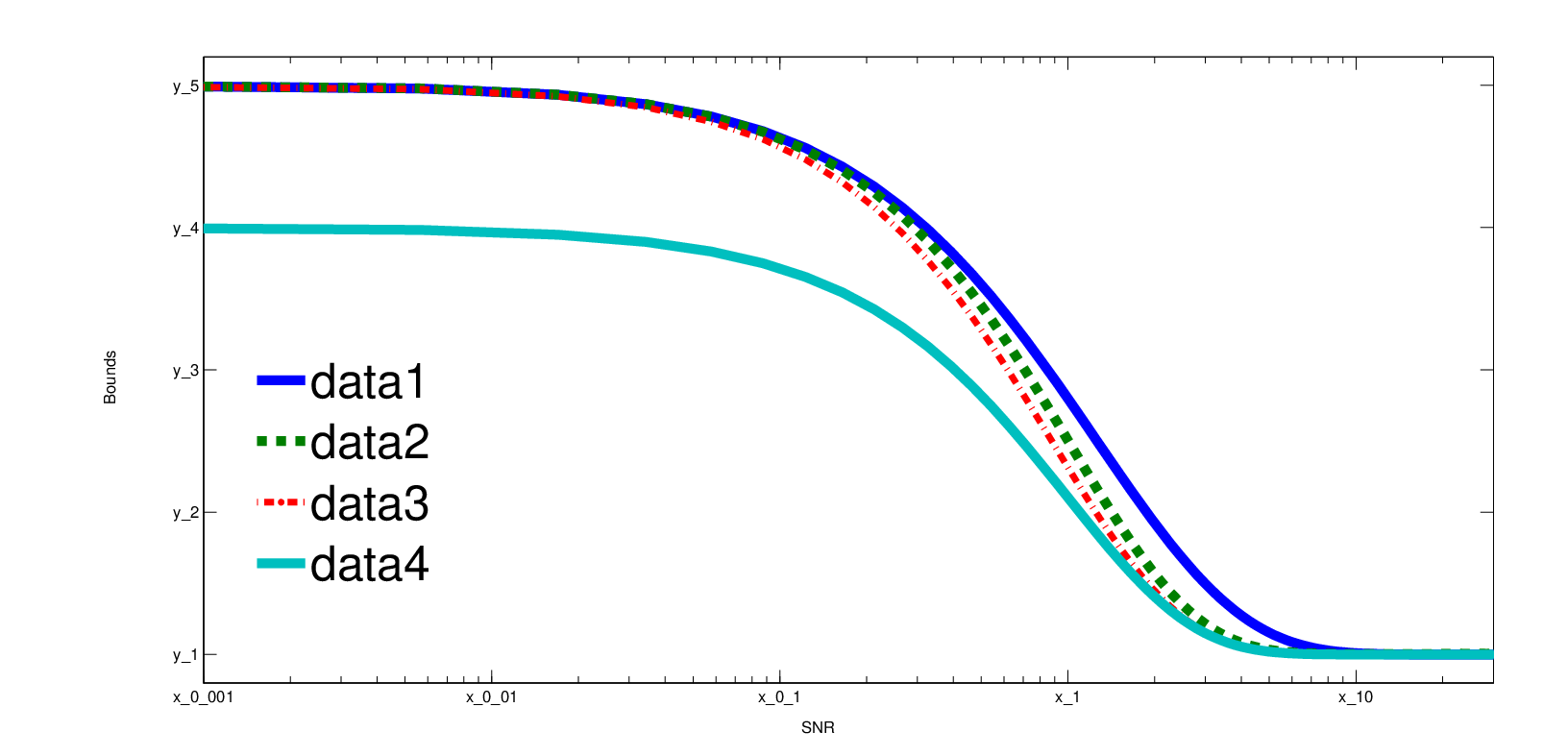
Fig. 1: Lower bounds HCRB​(𝐱)\mbox{HCRB}(\mathbf{x}), HCRB𝒱​(𝐱)\mbox{HCRB}_{\mathcal{V}}(\mathbf{x}) and upper bounds BBc​(𝐱)\mbox{BB}_{\text{c}}(\mathbf{x}), BBc′​(𝐱)\mbox{BB}^{\prime}_{\text{c}}(\mathbf{x}) on the MSE ε⁡(𝐱,𝐱^(𝐱))\varepsilon(\mathbf{x};\hat{\mathbf{x}}^{(\mathbf{x})}) of the LMVU estimator at 𝐱=c​(1  0  0  0  0)T\mathbf{x}=c\,(1\;\,0\;\,0\;\,0\;\,0)^{T}, with cc varied to obtain different values of SNR​(𝐱)=ξ2/σ2\mbox{SNR}(\mathbf{x})=\xi^{2}/\sigma^{2}. The SSNM parameters are N=5N\!=\!5, S=1S\!=\!1, and σ2=1\sigma^{2}\!=\!1.

For a parameter vector 𝐱\mathbf{x} with ‖𝐱‖0=S{\|\mathbf{x}\|}_{0}\!=\!S, let us reconsider the HCRB in (16). We will show that by using an increased number of appropriately chosen test points, we can obtain a lower bound that is higher (thus, tighter) than (19). Specifically, assume without loss of generality that supp⁡(𝐱)={1,…,S}\supp(\mathbf{x})=\{1,\ldots,S\}, and consider the set of test points

𝒱≜𝒱0∪⋃k=1S(𝒱k∪𝒲k)\mathcal{V}\,\triangleq\,\mathcal{V}_{0}\cup\,\bigcup_{k=1}^{S}(\mathcal{V}_{k}\cup\mathcal{W}_{k})\vskip-5.69054pt

with the component sets

𝒱0\displaystyle\mathcal{V}_{0} ≜⋃l∈supp⁡(𝐱){α​𝐞l}\displaystyle\,\triangleq\!\bigcup_{l\in\,\supp(\mathbf{x})}\!\{\alpha\hskip 0.56905pt\hskip 0.56905pt\mathbf{e}_{l}\}
𝒱k\displaystyle\mathcal{V}_{k} ≜⋃l∈{S+1,…,N}{α𝐞l−xk𝐞k},k=1,…,S\displaystyle\,\triangleq\!\bigcup_{l\in\{S+1,...,N\}}\!\{\alpha\hskip 0.56905pt\hskip 0.56905pt\mathbf{e}_{l}\hskip-0.56905pt-\hskip-0.56905ptx_{k}\hskip 0.56905pt\mathbf{e}_{k}\}\,,\qquad k=1,\ldots,S
𝒲k\displaystyle\mathcal{W}_{k} ≜⋃l∈{S+1,…,N}{xk𝐞l−xk𝐞k},k=1,…,S\displaystyle\,\triangleq\!\bigcup_{l\in\{S+1,...,N\}}\!\{x_{k}\hskip 0.56905pt\hskip 0.56905pt\mathbf{e}_{l}\hskip-0.56905pt-\hskip-0.56905ptx_{k}\hskip 0.56905pt\mathbf{e}_{k}\}\,,\qquad k=1,\ldots,S

where α=0.02​σ\alpha=0.02\hskip 0.56905pt\hskip 0.56905pt\sigma. In Fig. 1, the HCRB (16) for the new set 𝒱\mathcal{V} of test points—denoted HCRB𝒱​(𝐱)\mbox{HCRB}_{\mathcal{V}}(\mathbf{x})—is displayed versus the SNR and compared with HCRB​(𝐱)\mbox{HCRB}(\mathbf{x}). For this figure, we chose N​Ê=5NÊ\!=\!5, S=Ê​1S\!=Ê\!1, σ2=1\sigma^{2}\!=\!1, and 𝐱=c​(1  0  0  0  0)T\mathbf{x}=c\,(1\;\,0\;\,0\;\,0\;\,0)^{T}, where the parameter c∈ℝc\!\in\!\mathbb{R} is varied to obtain different SNR values.33 3 The use of a low-dimensional model is mandated by the complexity of the numerical approximation to the upper bound on the BB which will be described in Section V-B. As before, the SNR is defined as SNR​(𝐱)=ξ2/σ2\mbox{SNR}(\mathbf{x})=\xi^{2}/\sigma^{2}, where ξ\xi is the SS-largest (in magnitude) component of 𝐱{\bf x} (in our example with S=1S\!=\!1, ξ\xi is simply the single nonzero component). It can be seen from Fig. 1 that the numerical lower bound HCRB𝒱​(𝐱)\mbox{HCRB}_{\mathcal{V}}(\mathbf{x}) computed from the above test points is indeed tighter than the closed-form lower bound HCRB​(𝐱)\mbox{HCRB}(\mathbf{x}) in (19).

V-B Numerical Upper Bound

It is also possible to find upper bounds on the BB that are tighter (lower) than the upper bound BBc​(𝐱)\mbox{BB}_{\text{c}}(\mathbf{x}) in (28). Consider a parameter vector 𝐱\mathbf{x} with ‖𝐱‖0=S{\|\mathbf{x}\|}_{0}\!=\!S. We recall that BBc​(𝐱)\mbox{BB}_{\text{c}}(\mathbf{x}) was derived by constructing, for all k∉supp⁡(𝐱)k\notin\supp(\mathbf{x}), unbiased estimators x^k​(𝐲)=yk+x^k′​(𝐲)\hat{x}_{k}(\mathbf{y})=y_{k}+\hat{x}^{\prime}_{k}(\mathbf{y}) with x^k′​(𝐲)\hat{x}^{\prime}_{k}(\mathbf{y}) constrained by (23) and (24). We will now investigate how much we can improve on BBc​(𝐱)\mbox{BB}_{\text{c}}(\mathbf{x}) if we remove the constraint (23). Thus, in the optimization problem (22), the constraint set 𝒜𝐱\mathcal{A}_{\mathbf{x}} is hereafter considered to correspond only to the constraint (24).

In order to numerically solve this modified optimization problem (22), a discrete approximation for x^k′​(𝐲)\hat{x}^{\prime}_{k}({\bf y}) was used. More specifically, we defined x^k′​(𝐲)\hat{x}^{\prime}_{k}({\bf y}) to be piecewise constant in each of the components yly_{l} with l∈{k}∪supp⁡(𝐱)l\in\{k\}\cup\supp({\bf x}), and constant in the remaining components yly_{l} (the latter being required by (24)). We used QQ piecewise constant segments for each l∈{k}∪supp⁡(𝐱)l\in\{k\}\cup\supp({\bf x}), with each segment of length Δ=10​σ/Q\Delta\!=\!10\,\sigma/Q. These arrays of constant segments were centered about 𝐲=𝐱{\bf y}\!=\!{\bf x}. The remaining values of x^k′​(𝐲)\hat{x}^{\prime}_{k}({\bf y}) were set to 00. Thus, we obtained a function x^k′​(𝐲)\hat{x}^{\prime}_{k}({\bf y}) with linear dependence on a finite number QS+1Q^{S+1} of parameters. For functions of this form, the optimization problem (22) becomes a finite-dimensional quadratic program with linear constraints, which can be solved efficiently [29]. The MSE of the resulting estimator, denoted by BBc′​(𝐱)\mbox{BB}^{\prime}_{\text{c}}(\mathbf{x}), is an upper bound on the BB. This bound is tighter than the closed-form upper bound BBc​(𝐱)\mbox{BB}_{\text{c}}(\mathbf{x}) in (28) if QQ is large enough. In Fig. 1, we compare BBc′​(𝐱)\mbox{BB}^{\prime}_{\text{c}}(\mathbf{x}) for Q=20Q\!=\!20 with BBc​(𝐱)\mbox{BB}_{\text{c}}(\mathbf{x}) as a function of the SNR. The improved accuracy of BBc′​(𝐱)\mbox{BB}^{\prime}_{\text{c}}(\mathbf{x}) relative to BBc​(𝐱)\mbox{BB}_{\text{c}}(\mathbf{x}) is evident, particularly at high SNR values. Moreover, the proximity of the numerical upper bound BBc′​(𝐱)\mbox{BB}^{\prime}_{\text{c}}(\mathbf{x}) to the numerical lower bound HCRB𝒱​(𝐱)\mbox{HCRB}_{\mathcal{V}}(\mathbf{x}) indicates that these two bounds achieve an accurate characterization of the BB, since the BB lies between them.

V-C The Role of ξ\xi

We have seen in Section IV that for ‖𝐱‖0=S{\|\mathbf{x}\|}_{0}\!=\!S, the MSE of the LMVU estimator at high SNR is given by S​σ2S\sigma^{2}, and furthermore, convergence to this value is exponential in the quantity ξ2/σ2\xi^{2}/\sigma^{2}. A remarkable aspect of this conclusion is the fact that convergence to the high-SNR regime depends solely on ξ\xi, the smallest nonzero component of 𝐱{\bf x}, rather than having a more complex dependency on all the SS nonzero components of 𝐱{\bf x}. For example, one might imagine the behavior of an estimator to be rather different when all nonzero components have the same value ξ\xi, as opposed to the situation in which one component equals ξ\xi and the others are much larger. However, our analysis shows that when ξ≫σ\xi\hskip-0.56905pt\hskip-0.56905pt\gg\hskip-0.56905pt\hskip-0.56905pt\sigma, the remaining components of 𝐱{\bf x} have no effect on the performance of the LMVU estimator. We will next investigate whether practical estimators also exhibit such an effect.

Refer to caption
Fig. 2: MSE ε⁡(𝐱r,𝐱^ML)\varepsilon(\mathbf{x}_{r};\hat{\mathbf{x}}_{\text{ML}}) of the ML estimator for randomly generated parameter vectors 𝐱r\mathbf{x}_{r} at four different SNRs ξ2/σ2\xi^{2}/\sigma^{2}, for SSNM parameters N=10N\!=\!10, S=4S\!=\!4, and σ2=1\sigma^{2}\!=\!1.

To answer this question, we examined the MSE of the ML estimator (7) for a wide range of parameter vectors 𝐱{\bf x} having a predetermined smallest component ξ\xi. More specifically, for a given value of ξ\xi, we randomly generated 100100 parameter vectors 𝐱r\mathbf{x}_{r}, r=1,…,100r=1,\ldots,100, with 𝐱r∈𝒳S\mathbf{x}_{r}\!\!\in\!\mathcal{X}_{S} and ‖𝐱r‖0=S{\|\mathbf{x}_{r}\|}_{0}\!=\!S, whose minimum nonzero component was equal to ξ\xi. The other nonzero components were generated as independent, identically distributed realizations of the random variable x=ξ⁡(1+3​σ​|q|)x=\xi\hskip 0.56905pt(1+3\hskip 0.56905pt\sigma|q|), where q∼𝒩⁡(0,1)q\sim\mathcal{N}(0,1) is a standard Gaussian random variable and σ\sigma is the standard deviation of the noise. The MSE ε⁡(𝐱r,𝐱^ML)\varepsilon(\mathbf{x}_{r};\hat{\mathbf{x}}_{\text{ML}}) of the ML estimator is shown in Fig. 2 for N=10N\!=\!10, S=4S\!=\!4, and four different SNRs ξ2/σ2\xi^{2}/\sigma^{2}, with the horizontal axis representing the different choices of 𝐱r\mathbf{x}_{r} in arbitrary order. It is seen that for large ξ\xi, the performance of the ML estimator, like that of the LMVU, depends almost exclusively on ξ\xi. This suggests that the performance guarantees of Sections III and IV, while formally valid only for unbiased estimators, can still provide general conclusions which are relevant to biased techniques such as the ML estimator. Moreover, this result also justifies our definition of the SNR as the ratio ξ2/σ2\xi^{2}/\sigma^{2}, since this is the most significant factor determining estimation performance for the SSNM.

V-D Threshold Region Identification

In Sections III and  IV, we characterized the performance of unbiased estimators as a means of quantifying the difficulty of estimation for the SSNM. A common use of this analysis is in the identification of the threshold region, a range of SNR values which constitutes a transition between low-SNR and high-SNR behavior [30, 31, 32]. Specifically, in many cases the performance of estimators can be calculated analytically when the SNR is either very low or very high. It is then important to identify the threshold region which separates these two regimes. Although the analysis is based on bounds for unbiased estimators, the result is often heuristically assumed to approximate the threshold region for biased techniques as well [30, 32].

For ‖𝐱‖0=S{\|\mathbf{x}\|}_{0}\!=\!S, the lower and upper bounds on the BB (HCRB​(𝐱)\text{HCRB}(\mathbf{x}) in (19), BBc​(𝐱)\text{BB}_{\text{c}}(\mathbf{x}) in (28)) exhibit a transition between a low-SNR region, where both bounds are on the order of N​σ2N\sigma^{2}\hskip-0.56905pt, and a high-SNR region, for which both bounds converge to S​σ2S\sigma^{2}\hskip-0.56905pt. The BB therefore also displays such a transition. One can define the threshold region of the SSNM (for unbiased estimation) as the range of values of ξ2/σ2\mathbf{\xi}^{2}/\sigma^{2} in which this transition takes place. Since the BB is itself a lower bound on the performance of unbiased estimators, one would expect the transition region of actual estimators to occur at slightly higher SNR values than that of the BB.

To test this hypothesis, we compared the bounds of Sections III and  IV with the MSE of two well-known estimation schemes, namely, the ML estimator in (7) and the hard-thresholding (HT) estimator 𝐱^HT​(𝐲)\hat{\mathbf{x}}_{\text{HT}}(\mathbf{y}), which is given componentwise as

x^HT,k​(𝐲)={yk,|yk|≥T0,else\hat{x}_{\text{HT},k}(\mathbf{y})\,=\,\begin{cases}y_{k},&|y_{k}|\geq T\\[-2.84526pt] 0,&\text{else}\end{cases}

for a given threshold T>0T\!>\!0. In our simulations, we chose the commonly used value T=σ​2​log⁡NT=\sigma\sqrt{2\log{N}} [33]. Note that since the ML and HT estimators are biased, their MSE is not bounded by BBc​(𝐱)\mbox{BB}_{\text{c}}(\mathbf{x}), HCRB​(𝐱)\mbox{HCRB}(\mathbf{x}), and the CRB. Assuming SSNM parameters N=10N\!=\!10 and S=4S\!=4, we generated a number of parameter vectors 𝐱{\bf x} from the set ℛ≜{c​(1  1  1  1  0  0  0  0  0  0)T}c∈ℝ\mathcal{R}\triangleq\big\{c\,(1\;\,1\;\,1\;\,1\;\,0\;\,0\;\,0\;\,0\;\,0\;\,0)^{T}\big\}_{c\in\mathbb{R}}, where cc was varied to obtain a range of SNR values. For these 𝐱{\bf x}, we calculated the MSE of the two estimators 𝐱^ML\hat{\mathbf{x}}_{\text{ML}} and 𝐱^HT\hat{\mathbf{x}}_{\text{HT}} by means of numerical integration (see Appendix I for a discussion of the computation of ε⁡(𝐱,𝐱^ML)\varepsilon(\mathbf{x};\hat{\mathbf{x}}_{\text{ML}})).

The results are displayed in Fig. 3 as a function of the SNR ξ2/σ2\xi^{2}/\sigma^{2}. Although there is some gap between the lower bound (HCRB) and the upper bound (BBc\mbox{BB}_{\text{c}}), a rough indication of the behavior of the BB is conveyed. As expected, the threshold region exhibited by the ML and HT estimators is somewhat higher than that predicted by the bounds. Specifically, the threshold region of the BB (as indicated by the bounds) can be seen to occur at SNR values between −5-5 and 55 dB, while the threshold region of the ML and HT estimators is at SNR values between 55 and 1212 dB. Another effect which is visible in Fig. 3 is the convergence of the ML estimator to the BB at high SNR; this is a manifestation of the well-known fact that the ML estimator is asymptotically unbiased and asymptotically optimal. Finally, at low SNR, both the ML and HT estimators are better than the best unbiased approach. This is because unbiased methods generally perform poorly at low SNR, so that even the best unbiased technique is outperformed by the biased ML and HT estimators. On the other hand, for medium SNR, the MSE of the ML and HT estimators is significantly higher than the BB. Thus, there is a potential for unbiased estimators to perform better than biased estimators in the medium-SNR regime.

Refer to caption
Fig. 3: MSE of the ML and HT estimators compared with the performance bounds BBc​(𝐱)\mbox{BB}_{\text{c}}(\mathbf{x}), HCRB​(𝐱)\mbox{HCRB}(\mathbf{x}), and CRB (≡S​σ2\equiv S\sigma^{2}), as a function of the SNR ξ2/σ2\xi^{2}/\sigma^{2}, for SSNM parameters N=10N\!=\!10, S=4S\!=\!4, and σ2=1\sigma^{2}\!=\!1.
Refer to caption
Fig. 4: Ratio BBc​(𝐱)/HCRB​(𝐱)\mbox{BB}_{\text{c}}({\bf x})/\mbox{HCRB}({\bf x}) versus the SNR ξ2/σ2\xi^{2}/\sigma^{2} for different sets of parameter vectors 𝐱{\bf x}.

One may argue that considering only parameter vectors 𝐱{\bf x} in the set ℛ\mathcal{R} is not representative, since ℛ\mathcal{R} covers only a small part of the parameter space 𝒳S\mathcal{X}_{S}. However, the choice of ℛ\mathcal{R} is conservative in that the maximum deviation between HCRB​(𝐱)\mbox{HCRB}(\mathbf{x}) and BBc​(𝐱)\mbox{BB}_{\text{c}}(\mathbf{x}) is largest when the nonzero entries of 𝐱{\bf x} have approximately the same magnitude, which is the case for each element of ℛ\mathcal{R}. This is illustrated in Fig. 4, which shows the ratio between the two bounds versus the SNR ξ2/σ2\xi^{2}/\sigma^{2} for three different configurations of the nonzero entries in the parameter vector. Specifically, we considered the two additional sets ℛ2≜{c​(10  1  1  1  0  0  0  0  0  0)T}c∈ℝ\mathcal{R}_{2}\triangleq\big\{c\,(10\;\,1\;\,1\;\,1\;\,0\;\,0\;\,0\;\,0\;\,0\;\,0)^{T}\big\}_{c\in\mathbb{R}} and ℛ3≜{c​(0.1  1  1  1  0  0  0  0  0  0)T}c∈ℝ\mathcal{R}_{3}\triangleq\big\{c\,(0.1\;\,1\;\,1\;\,1\;\,0\;\,0\;\,0\;\,0\;\,0\;\,0)^{T}\big\}_{c\in\mathbb{R}}, in which the nonzero entries have different magnitudes. It can be seen from Fig. 4 that the ratio BBc​(𝐱)/HCRB​(𝐱)\mbox{BB}_{\text{c}}(\mathbf{x})/\mbox{HCRB}(\mathbf{x}) is indeed highest when 𝐱{\bf x} is in ℛ\mathcal{R}.

VI Conclusion

In this paper, we have studied unbiased estimation of a sparse vector in white Gaussian noise within a frequentist setting. As we have seen, without the assumption of sparsity, there exists only a single unbiased estimator. However, the addition of a sparsity assumption yields a rich family of unbiased estimators. The analysis of the performance of these estimators has been the primary goal of this paper. We first demonstrated that there exists no uniformly minimum variance unbiased estimator, i.e., no single unbiased estimator is optimal for all parameter values. Consequently, we focused on analyzing the Barankin bound (BB), i.e., the MSE of the locally minimum variance unbiased estimator, or equivalently, the smallest MSE achievable by an unbiased estimator for each value of the sparse vector.

For the sparse estimation problem considered, as for most estimation problems, the BB cannot be computed precisely. However, we demonstrated that it can be characterized quite accurately using numerical lower and upper bounds. Furthermore, we derived simple closed-form lower and upper bounds which are somewhat looser than the numerical bounds. These closed-form bounds allow an estimation of the threshold region separating the low-SNR and high-SNR regimes, and they indicate the asymptotic behavior of the BB at high SNR. In particular, a notable conclusion is that the high-SNR behavior of the BB depends solely on the value of the smallest nonzero component of the sparse vector.

While the unbiasedness property is intuitively appealing and related to several desirable asymptotic features of an estimator [6], one can often obtain biased estimators which outperform any unbiased estimator [13, 14, 15]. Thus, it is interesting to note that some of the conclusions obtained from our analysis of unbiased estimators appear to provide insight into the behavior of standard biased estimators. In particular, we saw that the behavior of two commonly used biased estimators at high SNR corresponds to the predictions of our unbiased bounds, not only in terms of the asymptotically achievable MSE but also in certain finer details, such as the SNR range of the threshold region and the fact that the convergence to the high-SNR regime depends primarily on the value of the smallest nonzero component of the sparse vector, rather than on the entire vector. This gives additional merit to the analysis of achievable estimation performance within the unbiased setting.

Appendix A Proof of Theorem 1

We wish to show that for S=NS\!=\!N, the only unbiased estimator with bounded MSE is the trivial estimator 𝐱^​(𝐲)=𝐲\hat{\mathbf{x}}(\mathbf{y})\hskip-0.56905pt=\hskip-0.56905pt\mathbf{y}. We will first show that a bounded MSE implies that 𝐱^​(𝐲)\hat{\mathbf{x}}(\mathbf{y}) is equivalent to a tempered distribution. This will allow us to reformulate the unbiasedness condition in the Fourier transform domain.

Using (3), the unbiasedness condition in (8) for S=NS\!=\!N

reads

1(2​π​σ2)N/2​∫ℝN𝐱^​(𝐲)​exp⁡(−12​σ2​‖𝐲−𝐱‖22)​𝑑𝐲=𝐱for all ​𝐱∈ℝN.\frac{1}{(2\pi\sigma^{2})^{N/2}}\int_{\mathbb{R}^{N}}\!\hat{\mathbf{x}}(\mathbf{y})\,\exp\hskip-0.56905pt\hskip-0.56905pt\bigg(\!\!-\frac{1}{2\sigma^{2}}\|\mathbf{y}\!-\!\mathbf{x}\|_{2}^{2}\bigg)\,d\mathbf{y}\,=\,\mathbf{x}\qquad\text{for all }\,\mathbf{x}\!\in\!\mathbb{R}^{N}\,.\vskip 2.84526pt (30)

The integral in (30) is the convolution of 𝐱^​(𝐲)\hat{\mathbf{x}}(\mathbf{y}) with exp⁡(−12​σ2​‖𝐲‖22)\exp\hskip-0.56905pt\hskip-0.56905pt\big(\!\!-\!\hskip-0.56905pt\frac{1}{2\sigma^{2}}\|\mathbf{y}\|_{2}^{2}\big). The result of this convolution, viewed as a function of 𝐱\mathbf{x}, must equal (2​π​σ2)N/2​𝐱(2\pi\sigma^{2})^{N/2}\,\mathbf{x} for all parameter vectors 𝐱\mathbf{x}. For absolutely integrable functions, the Fourier transform maps a convolution onto a pointwise product, and consequently it seems natural to consider the Fourier transform of condition (30) in order to simplify the analysis. However, typically, the estimator function 𝐱^​(𝐲)\hat{\mathbf{x}}(\mathbf{y}) will be neither absolutely integrable nor square integrable, and thus its Fourier transform can only exist in the sense of a tempered distribution [34]. From a practical point of view, the class of tempered distributions is large enough so that it does not exclude reasonable estimators such as the LS estimator (7). The following lemma states that 𝐱^​(𝐲)\hat{\mathbf{x}}(\mathbf{y}) can be viewed as a tempered distribution if it has a bounded MSE.

Lemma 9.

Consider an estimator 𝐱^\hat{\mathbf{x}} for the SSNM (2) with S=NS\!=\!N. If 𝐱^\hat{\mathbf{x}} has a bounded MSE, i.e., ε⁡(𝐱,𝐱^)≤C\varepsilon(\mathbf{x};\hat{\mathbf{x}})\leq C for all 𝐱∈ℝN\mathbf{x}\!\in\!\mathbb{R}^{N} (where CC is a constant which may depend on NN, SS, and σ2\sigma^{2}), then 𝐱^\hat{\mathbf{x}} is equivalent to a tempered distribution.

Proof. The proof of Lemma 9 is based on the following result which gives a sufficient condition for a function 𝐱^​(𝐲)\hat{\mathbf{x}}(\mathbf{y}) to be (equivalent to) a tempered distribution.

Proposition 10 ([34]).

If there exist constants B,n,R0∈ℝ+B,n,R_{0}\!\in\hskip-0.56905pt\hskip-0.56905pt\mathbb{R}_{+} such that

∫‖𝐲‖2≤R‖𝐱^​(𝐲)‖22​𝑑𝐲≤B​Rnfor all ​R≥R0\int_{{\|\mathbf{y}\|}_{2}\leq R}\|\hat{\mathbf{x}}(\mathbf{y})\|_{2}^{2}\,d\mathbf{y}\,\leq\,BR^{n}\quad\quad\text{for all }\,R\hskip-0.56905pt\geq\!R_{0} (31)

then 𝐱^​(𝐲)\hat{\mathbf{x}}(\mathbf{y}) is equivalent to a tempered distribution.

Let 𝐱^​(𝐲){\hat{{\bf x}}}({\bf y}) be an estimator function with bounded MSE, i.e., there exists a constant CC such that

𝖤𝐱​{‖𝐱^​(𝐲)−𝐱‖22}≤Cfor all ​𝐱∈𝒳S.\mathsf{E}_{\mathbf{x}}\{\|\hat{\mathbf{x}}(\mathbf{y})\hskip-0.56905pt-\hskip-0.56905pt\mathbf{x}\|_{2}^{2}\}\,\leq\,C\quad\quad\text{for all }\,\mathbf{x}\!\in\!\mathcal{X}_{S}\,. (32)

Defining the usual norm ∥⋅∥RV{\|\cdot\|}_{\rm RV} on the space of of random vectors by ‖𝐲‖RV≜𝖤𝐱​{‖𝐲‖22}\|\mathbf{y}\|_{\rm RV}\triangleq\sqrt{\mathsf{E}_{\mathbf{x}}\{\|\mathbf{y}\|^{2}_{2}\}}, we can use the (reverse) triangle inequality ‖𝐱^​(𝐲)−𝐱‖RV≥‖𝐱^​(𝐲)‖RV−‖𝐱‖RV{\|\hat{\mathbf{x}}(\mathbf{y})\!-\!\mathbf{x}\|}_{\rm RV}\geq{\|\hat{\mathbf{x}}(\mathbf{y})\|}_{\rm RV}-{\|\mathbf{x}\|}_{\rm RV} to

obtain

𝖤𝐱​{‖𝐱^​(𝐲)−𝐱‖22}≥𝖤𝐱​{‖𝐱^​(𝐲)‖22}−𝖤𝐱​{‖𝐱‖22}=𝖤𝐱​{‖𝐱^​(𝐲)‖22}−‖𝐱‖2.\sqrt{\mathsf{E}_{\mathbf{x}}\{\|\hat{\mathbf{x}}(\mathbf{y})\hskip-0.56905pt-\hskip-0.56905pt\mathbf{x}\|_{2}^{2}\}}\,\geq\,\sqrt{\mathsf{E}_{\mathbf{x}}\{\|\hat{\mathbf{x}}(\mathbf{y})\|_{2}^{2}\}}-\sqrt{\mathsf{E}_{\mathbf{x}}\{\|\mathbf{x}\|_{2}^{2}\}}\,=\,\sqrt{\mathsf{E}_{\mathbf{x}}\{\|\hat{\mathbf{x}}(\mathbf{y})\|_{2}^{2}\}}-{\|\mathbf{x}\|}_{2}\,.

From this, it follows

that

𝖤𝐱​{‖𝐱^​(𝐲)‖22}≤𝖤𝐱​{‖𝐱^​(𝐲)−𝐱‖22}+‖Ê​𝐱‖2≤C+‖Ê​𝐱‖2for all ​𝐱∈𝒳S,\sqrt{\mathsf{E}_{\mathbf{x}}\{\|\hat{\mathbf{x}}(\mathbf{y})\|_{2}^{2}\}}\,\leq\,\sqrt{\mathsf{E}_{\mathbf{x}}\{\|\hat{\mathbf{x}}(\mathbf{y})-\mathbf{x}\|_{2}^{2}\}}\hskip 0.56905pt+{\|Ê\mathbf{x}\|}_{2}\,\leq\,\sqrt{C}+{\|Ê\mathbf{x}\|}_{2}\qquad\text{for all }\,\mathbf{x}\!\in\!\mathcal{X}_{S}\,,

where (32) has been used. Squaring both sides and using the inequality (x+y)2≤2​(x2+y2)(x+y)^{2}\leq 2(x^{2}+y^{2}), we obtain

𝖤𝐱​{‖𝐱^​(𝐲)‖22}≤(C+‖Ê​𝐱‖2)2≤ 2​(C+‖Ê​𝐱‖22)for all ​𝐱∈𝒳S\mathsf{E}_{\mathbf{x}}\{\|\hat{\mathbf{x}}(\mathbf{y})\|_{2}^{2}\}\,\leq\,(\sqrt{C}+{\|Ê\mathbf{x}\|}_{2})^{2}\,\leq\,2\,(C+\|Ê\mathbf{x}\|_{2}^{2})\qquad\text{for all }\,\mathbf{x}\!\in\!\mathcal{X}_{S}\vskip-2.84526pt

or equivalently

1(2​π​σ2)N/2∫ℝN∥𝐱^(𝐲)∥22e−∥𝐲−𝐱∥22/(2σ2)d𝐲≤ 2(C+∥Ê𝐱∥22)for all 𝐱∈𝒳S.\frac{1}{(2\pi\sigma^{2})^{N/2}}\int_{\mathbb{R}^{N}}\!\|\hat{\mathbf{x}}(\mathbf{y})\|_{2}^{2}\,e^{-\|\mathbf{y}-\mathbf{x}\|_{2}^{2}/(2\sigma^{2})}\hskip 0.56905ptd\mathbf{y}\,\leq\,2\hskip 0.56905pt(C+\|Ê\mathbf{x}\|_{2}^{2})\quad\quad\text{for all }\,\mathbf{x}\!\in\!\mathcal{X}_{S}.\vskip 2.84526pt (33)

We will now show that (31) holds for R0=1R_{0}\hskip-0.56905pt\hskip-0.56905pt=\!1, i.e., R≥1R\hskip-0.56905pt\geq\!1. We define the NN-dimensional grid

𝒢≜{−m​Δ,−(m−1)​Δ,…,−Δ,0,Δ,…,m​Δ}N\mathcal{G}\,\triangleq\,\{-m\Delta,-(m\!-\!1)\Delta,\ldots,-\Delta,0,\Delta,\ldots,m\Delta\}^{\!N}

where 0<Δ≤R0<\Delta\leq R (hence, R/Δ≥1R/\Delta\geq 1) and m=⌊R/Δ⌋≤R/Δm=\lfloor R/\Delta\rfloor\leq R/\Delta. The number of grid points in any single dimension satisfies

2​m+1≤2​RΔ+12m\hskip-0.56905pt+\!1\,\leq\,\frac{2R}{\Delta}+1\vskip-5.69054pt (34)

so that

|𝒢|=(2​m+1)N≤(2​RΔ+1)N.|\mathcal{G}|\hskip 0.56905pt=\hskip 0.56905pt(2m\hskip-0.56905pt+\!1)^{N}\leq\hskip 0.56905pt\left(\frac{2R}{\Delta}+1\right)^{\!\hskip-0.56905ptN}\!. (35)

We thus

have

∑𝐱∈𝒢‖𝐱‖22\displaystyle\sum_{\mathbf{x}\in\mathcal{G}}\|\mathbf{x}\|_{2}^{2} =∑𝐱∈𝒢∑k=1Nxk2=∑k=1N∑𝐱∈𝒢xk2=∑k=1N[(2​m+1)N−1​∑l=−mm(l​Δ)2]=N​(2​m+1)N−1​∑l=−mm(l​Δ)2\displaystyle\hskip 0.56905pt=\sum_{\mathbf{x}\in\mathcal{G}}\sum_{k=1}^{N}x_{k}^{2}\,=\hskip 0.56905pt\sum_{k=1}^{N}\sum_{\mathbf{x}\in\mathcal{G}}\hskip-0.56905ptx_{k}^{2}\,=\hskip 0.56905pt\sum_{k=1}^{N}\Bigg[(2m\hskip-0.56905pt+\!1)^{N-1}\!\sum_{l=-m}^{m}\!(l\Delta)^{2}\Bigg]=\,N(2m\hskip-0.56905pt+\!1)^{N-1}\!\sum_{l=-m}^{m}\!(l\Delta)^{2}
Ê\displaystyle Ê ≤N(2m+1)N−1Δ2∫x=−R/ΔR/Δx2dx≤N(2​RΔ+1)N−123R3Δ\displaystyle\hskip 0.56905pt\leq\,N\hskip 0.56905pt(2m\hskip-0.56905pt+\!1)^{N-1}\Delta^{2}\!\int_{x=-R/\Delta}^{R/\Delta}\!x^{2}dx\,\leq\,N\!\left(\frac{2R}{\Delta}+1\right)^{\!\hskip-0.56905ptN-1}\frac{2}{3}\frac{R^{3}}{\Delta} (36)

where (34) was used in the last step. Furthermore, for c≜1(2​π​σ2)N/2e−NΔ2/(2σ2)c\hskip 0.56905pt\triangleq\frac{1}{(2\pi\sigma^{2})^{N/2}}e^{-N\Delta^{2}/(2\sigma^{2})}, we

have

1c1(2​π​σ2)N/2∑𝐱∈𝒢e−∥𝐲−𝐱∥22/(2σ2)≥1,for all 𝐲 with ‖𝐲‖2≤R\frac{1}{c}\,\frac{1}{(2\pi\sigma^{2})^{N/2}}\sum\limits_{\mathbf{x}\in\mathcal{G}}e^{-\|\mathbf{y}-\mathbf{x}\|_{2}^{2}/(2\sigma^{2})}\geq 1\,,\qquad\text{for all $\mathbf{y}$ with ${\|\mathbf{y}\|}_{2}\hskip-0.56905pt\leq\hskip-0.56905ptR$}\vskip 2.84526pt (37)

In order to verify this inequality, consider an arbitrary 𝐲∈ℝN\mathbf{y}\!\in\!\mathbb{R}^{N} with ‖𝐲‖2≤R{\|\mathbf{y}\|}_{2}\hskip-0.56905pt\leq\hskip-0.56905ptR. Since 0<Δ≤R0<\Delta\leq R, and since ‖𝐲‖2≤R{\|\mathbf{y}\|}_{2}\hskip-0.56905pt\leq\hskip-0.56905ptR implies that no component yky_{k} of 𝐲\mathbf{y} can be larger than RR, there always exists a grid point 𝐱~∈𝒢\tilde{\mathbf{x}}\!\in\!\mathcal{G} (dependent on 𝐲\mathbf{y}) such that |yk−x~k|≤Δ|y_{k}-\tilde{x}_{k}|\leq\Delta for all k∈{1,…,N}k\in\{1,\ldots,N\}. It follows that ‖𝐲−𝐱~‖22≤N​Δ2\|\mathbf{y}-\tilde{\mathbf{x}}\|^{2}_{2}\leq N\Delta^{2} and, in

turn,

e−NΔ2/(2σ2)≤e−∥𝐲−𝐱~∥22/(2σ2)≤∑𝐱∈𝒢e−∥𝐲−𝐱∥22/(2σ2),∥𝐲∥2≤Re^{-N\Delta^{2}/(2\sigma^{2})}\hskip 0.56905pt\leq\,e^{-\|\mathbf{y}-\tilde{\mathbf{x}}\|_{2}^{2}/(2\sigma^{2})}\hskip 0.56905pt\leq\hskip 0.56905pt\sum_{\mathbf{x}\in\mathcal{G}}e^{-\|\mathbf{y}-\mathbf{x}\|_{2}^{2}/(2\sigma^{2})}\,,\qquad{\|\mathbf{y}\|}_{2}\hskip-0.56905pt\leq\hskip-0.56905ptR\vskip-2.84526pt

which is equivalent to (37).

Successively using (37), (33), (35), (36), and 1≤2​R/Δ1\leq 2R/\Delta, we obtain the following sequence of inequalities:

∫‖𝐲‖2≤R‖𝐱^​(𝐲)‖22​𝑑𝐲\displaystyle\int_{{\|\mathbf{y}\|}_{2}\leq R}\|\hat{\mathbf{x}}(\mathbf{y})\|_{2}^{2}\,d\mathbf{y} ≤∫‖𝐲‖2≤R∥𝐱^(𝐲)∥22[1c1(2​π​σ2)N/2∑𝐱∈𝒢e−∥𝐲−𝐱∥22/(2σ2)]d𝐲\displaystyle\,\leq\,\int_{{\|\mathbf{y}\|}_{2}\leq R}\|\hat{\mathbf{x}}(\mathbf{y})\|_{2}^{2}\hskip 0.56905pt\bigg[\frac{1}{c}\,\frac{1}{(2\pi\sigma^{2})^{N/2}}\sum\limits_{\mathbf{x}\in\mathcal{G}}e^{-\|\mathbf{y}-\mathbf{x}\|_{2}^{2}/(2\sigma^{2})}\bigg]\,d\mathbf{y}
≤1c∑𝐱∈𝒢1(2​π​σ2)N/2∫ℝN∥𝐱^(𝐲)∥22e−∥𝐲−𝐱∥22/(2σ2)d𝐲\displaystyle\,\leq\,\frac{1}{c}\sum_{\mathbf{x}\in\mathcal{G}}\frac{1}{(2\pi\sigma^{2})^{N/2}}\int_{\mathbb{R}^{N}}\!\|\hat{\mathbf{x}}(\mathbf{y})\|_{2}^{2}\,e^{-\|\mathbf{y}-\mathbf{x}\|_{2}^{2}/(2\sigma^{2})}\hskip 0.56905ptd\mathbf{y}
≤1c​∑𝐱∈𝒢2​(C+‖𝐱‖22)\displaystyle\,\leq\,\frac{1}{c}\sum_{\mathbf{x}\in\mathcal{G}}2\hskip 0.56905pt(C+\|\mathbf{x}\|_{2}^{2})
Ê\displaystyle Ê ≤2c​[(2​RΔ+1)N​C+N​(2​RΔ+1)N−1​23​R3Δ]\displaystyle\,\leq\,\frac{2}{c}\bigg[\left(\frac{2R}{\Delta}+1\right)^{\!\hskip-0.56905ptN}\!\hskip-0.56905ptC+N\!\left(\frac{2R}{\Delta}+1\right)^{\!\hskip-0.56905ptN-1}\frac{2}{3}\frac{R^{3}}{\Delta}\bigg]
Ê\displaystyle Ê ≤2c​[(4​RΔ)N​C+N​(4​RΔ)N−1​23​R3Δ].\displaystyle\,\leq\,\frac{2}{c}\bigg[\left(\frac{4R}{\Delta}\right)^{\!\hskip-0.56905ptN}\!\hskip-0.56905ptC+N\!\left(\frac{4R}{\Delta}\right)^{\!\hskip-0.56905ptN-1}\frac{2}{3}\frac{R^{3}}{\Delta}\bigg]\,. (38)

It then follows from (38) that for

R≥1R\geq 1

∫‖𝐲‖2≤R‖𝐱^​(𝐲)‖22​𝑑𝐲\displaystyle\int_{{\|\mathbf{y}\|}_{2}\leq R}\|\hat{\mathbf{x}}(\mathbf{y})\|_{2}^{2}\,d\mathbf{y} ≤2c​[(4Δ)N​RN+2​C+N​(4Δ)N−1​23​RN+2Δ]\displaystyle\,\leq\,\frac{2}{c}\bigg[\left(\frac{4}{\Delta}\right)^{\!\hskip-0.56905ptN}\!\hskip-0.56905ptR^{N+2}\hskip 0.56905pt\hskip 0.56905ptC+N\!\left(\frac{4}{\Delta}\right)^{\!\hskip-0.56905ptN-1}\frac{2}{3}\frac{R^{N+2}}{\Delta}\bigg]
≤2c​RN+2ΔN​(4N​C+N​4N​23)\displaystyle\,\leq\,\frac{2}{c}\frac{R^{N+2}}{\Delta^{N}}\bigg(\hskip-0.56905pt4^{N}C+N4^{N}\frac{2}{3}\bigg)
=22​N+1c​ΔN​(C+2​N3)​RN+2.\displaystyle\,=\,\frac{2^{2N+1}}{c\,\Delta^{N}}\,\bigg(\hskip-0.56905ptC+\frac{2N}{3}\bigg)\,R^{N+2}\,.

Thus, we have established that under the conditions of Lemma 9 (bounded MSE), the bound (31) holds with R0=1R_{0}\hskip-0.56905pt=\!1, B=22​N+1c​ΔN​(C+2​N/3)B=\frac{2^{2N+1}}{c\,\Delta^{N}}\,(C+2N/3), and n=N+2n=N\hskip-0.56905pt+\hskip-0.56905pt2. Therefore, it follows from Proposition 10 that an estimator with bounded MSE is equivalent to a tempered distribution. This concludes the proof of Lemma 9. □\Box

We now continue our proof of Theorem 1. Any estimator 𝐱^​(𝐲)\hat{\mathbf{x}}(\mathbf{y}) for the SSNM (2) can be written as

𝐱^​(𝐲)=𝐲+𝐱^′​(𝐲)\hat{\mathbf{x}}(\mathbf{y})\hskip 0.56905pt=\hskip 0.56905pt\mathbf{y}+\hat{\mathbf{x}}^{\prime}(\mathbf{y}) (39)

with the correction term 𝐱^′​(𝐲)≜𝐱^​(𝐲)−𝐲\hat{\mathbf{x}}^{\prime}(\mathbf{y})\triangleq\hat{\mathbf{x}}(\mathbf{y})-\mathbf{y}. Because 𝖤𝐱​{𝐱^​(𝐲)}=𝖤𝐱​{𝐲}+𝖤𝐱​{𝐱^′​(𝐲)}=𝐱+𝖤𝐱​{𝐱^′​(𝐲)}\mathsf{E}_{\mathbf{x}}\{\hat{\mathbf{x}}(\mathbf{y})\}=\mathsf{E}_{\mathbf{x}}\{\mathbf{y}\}+\mathsf{E}_{\mathbf{x}}\{\hat{\mathbf{x}}^{\prime}(\mathbf{y})\}=\mathbf{x}+\mathsf{E}_{\mathbf{x}}\{\hat{\mathbf{x}}^{\prime}(\mathbf{y})\}, 𝐱^​(𝐲)\hat{\mathbf{x}}(\mathbf{y}) is unbiased if and only if

𝐛(𝐱;𝐱^)=𝖤𝐱{𝐱^′(𝐲)}≡1(2​π​σ2)N/2∫ℝN𝐱^′(𝐲)e−Ê∥𝐲−𝐱∥22/(2σ2)d𝐲= 0for all 𝐱∈𝒳S.\mathbf{b}(\mathbf{x};\hat{\mathbf{x}})\,=\,\mathsf{E}_{\mathbf{x}}\{\hat{\mathbf{x}}^{\prime}(\mathbf{y})\}\,\equiv\,\frac{1}{(2\pi\sigma^{2})^{N/2}}\int_{\mathbb{R}^{N}}\!\hat{\mathbf{x}}^{\prime}(\mathbf{y})\,e^{-Ê\|\mathbf{y}-\mathbf{x}\|^{2}_{2}/(2\sigma^{2})}\hskip 0.56905ptd\mathbf{y}\,=\,\mathbf{0}\qquad\text{for all }\,\mathbf{x}\!\in\!\mathcal{X}_{S}\,.\vskip 2.84526pt (40)

Remember that we assume that 𝐱^\hat{\mathbf{x}} has a bounded MSE, so that according to our above proof of Lemma 9, the estimator function 𝐱^​(𝐲)\hat{\mathbf{x}}(\mathbf{y}) satisfies condition (31) with n=N+2n=N+2, i.e.,

∫‖𝐲‖2≤R‖𝐱^​(𝐲)‖22​𝑑𝐲≤B​RN+2for all​R≥1\int_{{\|\mathbf{y}\|}_{2}\,\leq\,R}{\|\hat{\mathbf{x}}(\mathbf{y})\|}_{2}^{2}\,d\mathbf{y}\,\leq\,BR^{N+2}\qquad\text{for all}\;\,R\hskip-0.56905pt\geq\hskip-0.56905pt\hskip-0.56905pt1\vskip 1.99168pt (41)

with BB as given at the end of the proof of Lemma 9. We will also need the following bound, in which ℛ≜[−R,R]N\mathcal{R}\triangleq[-R,R]^{N}:

∫‖𝐲‖2≤R‖𝐲‖22​𝑑𝐲≤∫ℛ‖𝐲‖22​𝑑𝐲=∑k=1N∫ℛyk2​𝑑𝐲=∑k=1N(2​R)N−1​23​R3=N3​2N​RN+2.\int_{{\|\mathbf{y}\|}_{2}\leq R}\|\mathbf{y}\|_{2}^{2}\,d\mathbf{y}\,\leq\int_{\mathcal{R}}\|\mathbf{y}\|_{2}^{2}\,d\mathbf{y}\,=\hskip 0.56905pt\sum_{k=1}^{N}\int_{\mathcal{R}}y_{k}^{2}\,d\mathbf{y}\,=\hskip 0.56905pt\sum_{k=1}^{N}(2R)^{N-1}\,\frac{2}{3}\hskip 0.56905pt\hskip 0.56905ptR^{3}\,=\,\frac{N}{3}\hskip 0.56905pt2^{N}\hskip-0.56905ptR^{N+2}\,.\vskip 2.84526pt (42)

We then have for the correction term 𝐱^′​(𝐲)\hat{\mathbf{x}}^{\prime}(\mathbf{y}), for all R≥1R\hskip-0.56905pt\geq\hskip-0.56905pt1,

∫‖𝐲‖2≤R‖𝐱^′​(𝐲)‖22​𝑑𝐲\displaystyle\int_{{\|\mathbf{y}\|}_{2}\leq R}\|\hat{\mathbf{x}}^{\prime}(\mathbf{y})\|_{2}^{2}\,d\mathbf{y} =∫‖𝐲‖2≤R‖𝐱^​(𝐲)−𝐲‖22​𝑑𝐲\displaystyle\,=\int_{{\|\mathbf{y}\|}_{2}\leq R}\|\hat{\mathbf{x}}(\mathbf{y})-\mathbf{y}\|_{2}^{2}\,d\mathbf{y}
≤∫‖𝐲‖2≤R2​(‖𝐱^​(𝐲)‖22+‖𝐲‖22)​𝑑𝐲\displaystyle\,\leq\,\int_{{\|\mathbf{y}\|}_{2}\leq R}2\hskip 0.56905pt\big(\|\hat{\mathbf{x}}(\mathbf{y})\|_{2}^{2}+\|\mathbf{y}\|_{2}^{2}\big)\hskip 0.56905ptd\mathbf{y}
= 2​(∫‖𝐲‖2≤R‖𝐱^​(𝐲)‖22​𝑑𝐲+∫‖𝐲‖2≤R‖𝐲‖22​𝑑𝐲)\displaystyle\,=\,2\hskip 0.56905pt\hskip 0.56905pt\Bigg(\int_{{\|\mathbf{y}\|}_{2}\leq R}\|\hat{\mathbf{x}}(\mathbf{y})\|_{2}^{2}\,d\mathbf{y}\,+\int_{{\|\mathbf{y}\|}_{2}\leq R}\|\mathbf{y}\|_{2}^{2}\,d\mathbf{y}\Bigg)
Ê\displaystyle Ê ≤ 2​(B​RN+2+N3​2N​RN+2)\displaystyle\,\leq\,2\hskip 0.56905pt\hskip 0.56905pt\bigg(BR^{N+2}\,+\,\frac{N}{3}\hskip 0.56905pt2^{N}\hskip-0.56905ptR^{N+2}\bigg)
Ê\displaystyle Ê =(2​B+N3​2N+1)​RN+2\displaystyle\,=\,\bigg(2B+\frac{N}{3}2^{N+1}\bigg)\hskip 0.56905ptR^{N+2}

where (41) and (42) have been used. Therefore, the correction term 𝐱^′​(𝐲)\hat{\mathbf{x}}^{\prime}(\mathbf{y}) also satisfies (31) and thus, according to Proposition 10, it is equivalent to a tempered distribution.

The bias function 𝐛⁡(𝐱,𝐱^)\mathbf{b}(\mathbf{x},\hat{\mathbf{x}}) in (40) is the convolution of 𝐱^′​(𝐲)\hat{\mathbf{x}}^{\prime}(\mathbf{y}) with the Gaussian function (2πσ2)−N/2e−∥𝐲∥22/(2σ2)(2\pi\sigma^{2})^{-N/2}\,e^{-\|\mathbf{y}\|^{2}_{2}/(2\sigma^{2})}. Because S=NS\!=\!N, we have 𝒳S=ℝN\mathcal{X}_{S}\!=\!\mathbb{R}^{N}, and thus (40) holds for all 𝐱∈ℝN\mathbf{x}\!\in\!\mathbb{R}^{N}. Since 𝐱^′​(𝐲)\hat{\mathbf{x}}^{\prime}(\mathbf{y}) is a tempered distribution and the Gaussian function is in the Schwartz class, it follows that the Fourier transform of the convolution product (40) is a smooth function which can be calculated as the pointwise product 𝐱¯′(𝐲¯)e−∥𝐲¯∥22/(2σ2)\bar{\mathbf{x}}^{\prime}(\bar{\mathbf{y}})\,e^{-\|\bar{\mathbf{y}}\|^{2}_{2}/(2\sigma^{2})}, where 𝐱¯′​(𝐲¯)\bar{\mathbf{x}}^{\prime}(\bar{\mathbf{y}}) denotes the Fourier transform of 𝐱^′​(𝐲)\hat{\mathbf{x}}^{\prime}(\mathbf{y}) [34]. Therefore, (40) is equivalent to 𝐱¯′(𝐲¯)e−∥𝐲¯∥22/(2σ2)=𝟎\bar{\mathbf{x}}^{\prime}(\bar{\mathbf{y}})\,e^{-\|\bar{\mathbf{y}}\|^{2}_{2}/(2\sigma^{2})}=\mathbf{0} for all 𝐲¯∈ℝN\bar{\mathbf{y}}\!\in\!\mathbb{R}^{N}. This can only be satisfied if 𝐱¯′​(𝐲¯)≡𝟎\bar{\mathbf{x}}^{\prime}(\bar{\mathbf{y}})\equiv\mathbf{0}, which in turn implies that 𝐱^′​(𝐲)≡𝟎\hat{\mathbf{x}}^{\prime}(\mathbf{y})\equiv\mathbf{0} (up to deviations of zero measure) and further, by (39), that 𝐱^​(𝐲)=𝐲\hat{\mathbf{x}}(\mathbf{y})=\mathbf{y}. Recalling that 𝒳S=ℝN\mathcal{X}_{S}\!=\!\mathbb{R}^{N}, it is clear from (5) that 𝐱^​(𝐲)=𝐲\hat{\mathbf{x}}(\mathbf{y})=\mathbf{y} is the LS estimator. Thus, we have shown that 𝐱^LS​(𝐲)=𝐲\hat{\mathbf{x}}_{\text{LS}}(\mathbf{y})=\mathbf{y} is the unique unbiased estimator for the SSNM with S=NS\!=\!N.

Appendix B Proof of Theorem 3

We must show that there exists no UMVU estimator for the SSNM with S<NS\!<\!N. The outline of our proof is as follows. We first demonstrate that the unique solution of the optimization problem (11) at the parameter value 𝐱=𝟎\mathbf{x}\!=\!{\boldsymbol{0}}, i.e., arg​min𝐱^​(⋅)∈𝒰⁡V​(𝟎,𝐱^)\argmin_{\hat{\mathbf{x}}(\cdot)\hskip 0.56905pt\in\,\mathcal{U}}V({\boldsymbol{0}};\hat{\mathbf{x}}), is the estimator 𝐱^(𝟎)​(𝐲)=𝐲{\hat{{\bf x}}}^{({\boldsymbol{0}})}({\bf y})={\bf y}. We then show that there exist unbiased estimators which have lower variance than 𝐱^(𝟎){\hat{{\bf x}}}^{({\boldsymbol{0}})} at other points 𝐱\mathbf{x}. This implies that neither 𝐱^(𝟎){\hat{{\bf x}}}^{({\boldsymbol{0}})} nor any other estimator uniformly minimizes the variance for all 𝐱\mathbf{x} among all unbiased estimators.

The estimator 𝐱^(𝟎)​(𝐲)=𝐲{\hat{{\bf x}}}^{({\boldsymbol{0}})}({\bf y})={\bf y} is a solution of (11) when 𝐱=𝟎\mathbf{x}\!=\!{\boldsymbol{0}} because the minimum variance at 𝐱=𝟎\mathbf{x}=\mathbf{0} of any unbiased estimator is bounded below by N​σ2N\sigma^{2} and 𝐱^(𝟎)​(𝐲)=𝐲\hat{\mathbf{x}}^{(\mathbf{0})}({\bf y})=\mathbf{y} achieves this lower bound [21]. To show that 𝐱^(𝟎)\hat{\mathbf{x}}^{(\mathbf{0})} is the unique solution of (11) for 𝐱=𝟎\mathbf{x}\!=\!\mathbf{0}, suppose by contradiction that there exists a second unbiased estimator 𝐱^a\hat{\mathbf{x}}_{a} different from 𝐱^(𝟎)\hat{\mathbf{x}}^{(\mathbf{0})}, also having variance N​σ2N\sigma^{2} at 𝐱=𝟎\mathbf{x}\!=\!\mathbf{0}. Consider the estimator 𝐱^new≜(𝐱^(𝟎)+𝐱^a)/2{\hat{{\bf x}}}_{\text{new}}\triangleq({\hat{{\bf x}}}^{({\boldsymbol{0}})}+\hat{\mathbf{x}}_{a})/2. Since 𝐱^(𝟎){\hat{{\bf x}}}^{({\boldsymbol{0}})} and 𝐱^a\hat{\mathbf{x}}_{a} are unbiased, 𝐱^new{\hat{{\bf x}}}_{\text{new}} is unbiased as well. Thus, its variance is (see (4)) V⁡(𝐱,𝐱^new)=P⁡(𝐱,𝐱^new)−‖𝐱‖22V(\mathbf{x};{\hat{{\bf x}}}_{\text{new}})=P(\mathbf{x};{\hat{{\bf x}}}_{\text{new}})-\|\mathbf{x}\|^{2}_{2}. In particular, we obtain for

𝐱=𝟎\mathbf{x}\!=\!\mathbf{0}

V⁡(𝟎,𝐱^new)\displaystyle V(\mathbf{0};{\hat{{\bf x}}}_{\text{new}}) =P⁡(𝟎,𝐱^new)=𝖤𝐱=𝟎​{‖12​(𝐱^(𝟎)+𝐱^a)‖22}\displaystyle\,=\,P(\mathbf{0};{\hat{{\bf x}}}_{\text{new}})\,=\,\mathsf{E}_{\mathbf{x}={\boldsymbol{0}}}\bigg\{\bigg\|\frac{1}{2}\hskip 0.56905pt({\hat{{\bf x}}}^{({\boldsymbol{0}})}\hskip-0.56905pt+\hat{\mathbf{x}}_{a})\bigg\|^{2}_{2}\bigg\}
=14​[𝖤𝐱=𝟎​{‖𝐱^(𝟎)‖22}+𝖤𝐱=𝟎​{‖𝐱^a‖22}+2​𝖤𝐱=𝟎​{(𝐱^(𝟎))T​𝐱^a}]\displaystyle\,=\,\frac{1}{4}\hskip 0.56905pt\big[\,\mathsf{E}_{\mathbf{x}={\boldsymbol{0}}}\big\{\|{\hat{{\bf x}}}^{({\boldsymbol{0}})}\|^{2}_{2}\big\}+\mathsf{E}_{\mathbf{x}={\boldsymbol{0}}}\big\{\|\hat{\mathbf{x}}_{a}\|^{2}_{2}\big\}+2\,\mathsf{E}_{\mathbf{x}={\boldsymbol{0}}}\big\{({\hat{{\bf x}}}^{({\boldsymbol{0}})})^{T}\hat{\mathbf{x}}_{a}\big\}\hskip 0.56905pt\big]
<(∗)14​[𝖤𝐱=𝟎​{‖𝐱^(𝟎)‖22}+𝖤𝐱=𝟎​{‖𝐱^a‖22}+2​𝖤𝐱=𝟎​{‖𝐱^(𝟎)‖22}​𝖤𝐱=𝟎​{‖𝐱^a‖22}]\displaystyle\stackrel{{\scriptstyle(*)}}{{\,<\,}}\frac{1}{4}\hskip 0.56905pt\Big[\,\mathsf{E}_{\mathbf{x}={\boldsymbol{0}}}\big\{\|{\hat{{\bf x}}}^{({\boldsymbol{0}})}\|^{2}_{2}\big\}+\mathsf{E}_{\mathbf{x}={\boldsymbol{0}}}\big\{\|\hat{\mathbf{x}}_{a}\|^{2}_{2}\big\}+2\sqrt{\mathsf{E}_{\mathbf{x}={\boldsymbol{0}}}\big\{\|{\hat{{\bf x}}}^{({\boldsymbol{0}})}\|^{2}_{2}\big\}\hskip 0.56905pt\mathsf{E}_{\mathbf{x}={\boldsymbol{0}}}\big\{\|\hat{\mathbf{x}}_{a}\|^{2}_{2}\big\}}\,\hskip 0.56905pt\Big]
=14⋅4​N​σ2=N​σ2\displaystyle\,=\,\frac{1}{4}\hskip-0.56905pt\cdot 4\hskip 0.56905ptN\sigma^{2}\hskip-0.56905pt\,=\,N\sigma^{2}

where the strict inequality (∗)(*) follows from the Cauchy-Schwarz inequality applied to the inner product 𝖤𝐱=𝟎​{(𝐱^(𝟎))T​𝐱^a}\mathsf{E}_{\mathbf{x}={\boldsymbol{0}}}\big\{({\hat{{\bf x}}}^{({\boldsymbol{0}})})^{T}\hat{\mathbf{x}}_{a}\big\}, combined with the fact that 𝐱^(𝟎)\hat{\mathbf{x}}^{(\mathbf{0})} and 𝐱^a\hat{\mathbf{x}}_{a} are not linearly dependent (indeed, 𝐱^a≠c​𝐱^(𝟎)\hat{\mathbf{x}}_{a}\not=c\hskip 0.56905pt\hat{\mathbf{x}}^{(\mathbf{0})} since 𝐱^(𝟎)\hat{\mathbf{x}}^{(\mathbf{0})} and 𝐱^a\hat{\mathbf{x}}_{a} were assumed to be different unbiased estimators). This inequality means that the variance of 𝐱^new{\hat{{\bf x}}}_{\text{new}} at 𝐱=𝟎\mathbf{x}\!=\!{\boldsymbol{0}} is lower than N​σ2N\sigma^{2}. But this is impossible, as N​σ2N\sigma^{2} is the minimum variance at 𝐱=𝟎\mathbf{x}\!=\!\mathbf{0} achieved by any unbiased estimator. Thus, we have shown that 𝐱^(𝟎)\hat{\mathbf{x}}^{(\mathbf{0})} is the unique solution of (11) for 𝐱=𝟎\mathbf{x}\!=\!\mathbf{0}.

Next, still for S<NS\!<\!N, we consider the specific parameter value 𝐱′∈𝒳S\mathbf{x}^{\prime}\!\hskip-0.56905pt\in\!\mathcal{X}_{S} whose components are given

by

xk′={1,k=2,…,S+1,0,else.x^{\prime}_{k}\,=\hskip 0.56905pt\begin{cases}1\hskip 0.56905pt,&k=2,\ldots,S\!+\!1\hskip 0.56905pt,\\[-2.84526pt] 0\hskip 0.56905pt,&\text{else}\hskip 0.56905pt.\end{cases}

The estimator 𝐱^(𝟎)\hat{\mathbf{x}}^{(\mathbf{0})} has variance V⁡(𝐱′,𝐱^(𝟎))=Ê​N​σ2V(\mathbf{x}^{\prime};\hat{\mathbf{x}}^{(\mathbf{0})})\!=Ê\!N\sigma^{2} at 𝐱′\mathbf{x}^{\prime} (and at all other 𝐱∈𝒳S\mathbf{x}\!\in\!\mathcal{X}_{S}). We will now construct an unbiased estimator 𝐱^b​(𝐲)\hat{\mathbf{x}}_{b}(\mathbf{y}) whose variance at 𝐱′\mathbf{x}^{\prime} is smaller than N​σ2N\sigma^{2}. The components of this estimator are defined as

x^b,k​(𝐲)≜Ê​{y1+A​y1​∏l=2S+1h⁡(yl),k=1yk,k=2,…,N\hat{x}_{b,k}(\mathbf{y})\,\triangleq Ê\begin{cases}y_{1}+A\hskip 0.56905pty_{1}\prod_{l=2}^{S+1}h(y_{l})\hskip 0.56905pt,&k=1\\[-2.84526pt] y_{k}\,,&k=2,\ldots,N\end{cases}\vskip-2.84526pt (43)

where

h⁡(y)≜{sgn​(y),|y|∈[0.4,0.6]0,elseh(y)\,\triangleq\hskip 0.56905pt\begin{cases}\mbox{sgn}(y)\hskip 0.56905pt,&|y|\in[0.4,0.6]\\[-2.84526pt] 0\hskip 0.56905pt,&\mbox{else}\end{cases}

and A∈ℝA\!\in\!\mathbb{R} is a parameter to be determined shortly.44 4 The interval [0.4,0.6][0.4,0.6] in the definition of h⁡(y)h(y) is chosen rather arbitrarily. Any interval which ensures that β\beta in (44) is nonzero can be used. A direct calculation shows that 𝐱^b​(𝐲)\hat{\mathbf{x}}_{b}(\mathbf{y}) is unbiased for all 𝐱∈𝒳S\mathbf{x}\!\in\!\mathcal{X}_{S}. Note that 𝐱^b​(𝐲)\hat{\mathbf{x}}_{b}(\mathbf{y}) is identical to 𝐱^(𝟎)​(𝐲)=𝐲\hat{\mathbf{x}}^{(\mathbf{0})}({\bf y})={\bf y} except for the first component, x^b,1​(𝐲)\hat{x}_{b,1}(\mathbf{y}).

We recall that for unbiased estimators, minimizing the variance V⁡(𝐱,𝐱^)V(\mathbf{x};\hat{\mathbf{x}}) is equivalent to minimizing the mean power P⁡(𝐱,𝐱^)=𝖤𝐱​{‖𝐱^​(𝐲)‖22}P(\mathbf{x};\hat{\mathbf{x}})=\mathsf{E}_{\mathbf{x}}\big\{\|\hat{\mathbf{x}}(\mathbf{y})\|^{2}_{2}\big\} (see (4)); furthermore, P⁡(𝐱,𝐱^)=∑k=1NP⁡(𝐱,x^k)P(\mathbf{x};\hat{\mathbf{x}})=\sum_{k=1}^{N}P(\mathbf{x};\hat{x}_{k}) with P⁡(𝐱,x^k)≜𝖤𝐱​{(x^k​(𝐲))2}P(\mathbf{x};\hat{x}_{k})\triangleq\mathsf{E}_{\mathbf{x}}\big\{(\hat{x}_{k}(\mathbf{y}))^{2}\big\}. For the proposed estimator 𝐱^b\hat{\mathbf{x}}_{b}, P⁡(𝐱′,x^b,k)=P⁡(𝐱′,x^k(𝟎))P(\mathbf{x}^{\prime};\hat{x}_{b,k})=P\big(\mathbf{x}^{\prime};\hat{x}_{k}^{(\mathbf{0})}\big) except for k=1k\!=\!1. Therefore, our goal is to choose AA such that P⁡(𝐱′,x^b,1)P(\mathbf{x}^{\prime};\hat{x}_{b,1}) is smaller than P⁡(𝐱′,x^1(𝟎))=σ2+(x1′)2=σ2P\big(\mathbf{x}^{\prime};\hat{x}_{1}^{(\mathbf{0})}\big)=\sigma^{2}+(x^{\prime}_{1})^{2}=\sigma^{2}. We

have

P⁡(𝐱′,x^b,1)=𝖤𝐱′​{(y1+A​y1​∏l=2S+1h⁡(yl))2}=α​A2+β​A+γP(\mathbf{x}^{\prime};\hat{x}_{b,1})\,=\,\mathsf{E}_{\mathbf{x}^{\prime}}\hskip-0.56905pt\Bigg\{\hskip-0.56905pt\Bigg(\hskip 0.56905pty_{1}+A\hskip 0.56905pty_{1}\prod_{l=2}^{S+1}h(y_{l})\Bigg)^{\!\!2}\hskip 0.56905pt\Bigg\}\,=\,\alpha\hskip 0.56905ptA^{2}+\hskip 0.56905pt\beta\hskip 0.56905ptA\hskip 0.56905pt+\hskip 0.56905pt\gamma (44)

with

α=𝖤𝐱′​{y12​∏l=2S+1h2​(yl)},β=𝖤𝐱′​{2​y12​∏l=2S+1h⁡(yl)},γ=𝖤𝐱′​{y12}=σ2.\alpha\hskip 0.56905pt=\hskip 0.56905pt\mathsf{E}_{\mathbf{x}^{\prime}}\hskip-0.56905pt\Bigg\{y_{1}^{2}\prod_{l=2}^{S+1}h^{2}(y_{l})\Bigg\}\,,\qquad\beta\hskip 0.56905pt=\hskip 0.56905pt\mathsf{E}_{\mathbf{x}^{\prime}}\hskip-0.56905pt\Bigg\{2\hskip 0.56905pty_{1}^{2}\prod_{l=2}^{S+1}h(y_{l})\Bigg\}\,,\qquad\gamma\hskip 0.56905pt=\hskip 0.56905pt\mathsf{E}_{\mathbf{x}^{\prime}}\hskip-0.56905pt\big\{y_{1}^{2}\big\}\hskip 0.56905pt=\hskip 0.56905pt\sigma^{2}.\vskip 2.84526pt

Note that γ=P⁡(𝐱′,x^1(𝟎))\gamma=P\big(\mathbf{x}^{\prime};\hat{x}_{1}^{(\mathbf{0})}\big). From (44), the AA minimizing P⁡(𝐱′,x^b,1)P(\mathbf{x}^{\prime};\hat{x}_{b,1}) is obtained as −β/(2α)-\beta/(2\alpha); the associated minimum P⁡(𝐱′,x^b,1)P(\mathbf{x}^{\prime};\hat{x}_{b,1}) is given by γ−β2/(4​α2)\gamma-\beta^{2}/(4\alpha^{2}). It can be shown that β\beta is nonzero due to the construction of h⁡(y)h(y). It follows that β\beta is positive, and therefore P⁡(𝐱′,x^b,1)P(\mathbf{x}^{\prime};\hat{x}_{b,1}) is smaller than γ=P⁡(𝐱′,x^1(𝟎))\gamma=P\big(\mathbf{x}^{\prime};\hat{x}_{1}^{(\mathbf{0})}\big). Thus, using A=−β/(2α)A=-\beta/(2\alpha) in (43), we obtain an estimator 𝐱^b\hat{\mathbf{x}}_{b} which has a smaller component power P⁡(𝐱′,x^b,1)P(\mathbf{x}^{\prime};\hat{x}_{b,1}) than 𝐱^(𝟎)\hat{\mathbf{x}}^{(\mathbf{0})}. Since P⁡(𝐱′,x^b,k)=P⁡(𝐱′,x^k(𝟎))P(\mathbf{x}^{\prime};\hat{x}_{b,k})=P\big(\mathbf{x}^{\prime};\hat{x}_{k}^{(\mathbf{0})}\big) for k=2,…,Nk=2,\ldots,N, it follows that the overall mean power of 𝐱^b\hat{\mathbf{x}}_{b} at 𝐱′\mathbf{x}^{\prime} is smaller than that of 𝐱^(𝟎)\hat{\mathbf{x}}^{(\mathbf{0})}, i.e., P⁡(𝐱′,𝐱^b)<P⁡(𝐱′,𝐱^(𝟎))P(\mathbf{x}^{\prime};\hat{\mathbf{x}}_{b})<P(\mathbf{x}^{\prime};\hat{\mathbf{x}}^{(\mathbf{0})}). Since both estimators are unbiased, this moreover implies that at 𝐱′\mathbf{x}^{\prime}, the variance of 𝐱^b\hat{\mathbf{x}}_{b} is smaller than that of 𝐱^(𝟎)\hat{\mathbf{x}}^{(\mathbf{0})}. Thus, 𝐱^(𝟎)\hat{\mathbf{x}}^{(\mathbf{0})} cannot be the LMVU estimator at 𝐱=𝐱′\mathbf{x}\!=\!\mathbf{x}^{\prime}. On the other hand, as we have seen, 𝐱^(𝟎)\hat{\mathbf{x}}^{(\mathbf{0})} is the unique LMVU estimator at 𝐱=𝟎\mathbf{x}\!=\!\mathbf{0}. We conclude that there does not exist a single unbiased estimator which simultaneously minimizes the variance for all parameters 𝐱∈𝒳S\mathbf{x}\!\in\!\mathcal{X}_{S}.

Appendix C Proof of Proposition 4

We begin by stating the multivariate HCRB.

Proposition 11 (Gorman and Hero [23]).

Let f⁡(𝐲,𝐱)f({\bf y};{\bf x}) be a family of pdf’s of 𝐲{\bf y} indexed by 𝐱∈𝒳S{\bf x}\!\in\!{\mathcal{X}_{S}}, and let 𝐱+𝐯1,…,𝐱+𝐯p{\bf x}+{\bf v}_{1},\ldots,{\bf x}+{\bf v}_{p} be a set of points in 𝒳S{\mathcal{X}_{S}}. Given an estimator 𝐱^{\hat{{\bf x}}}, define

𝐦𝐱\displaystyle{\bf m}_{\bf x} ≜𝖤𝐱​{𝐱^}\displaystyle\,\triangleq\,\mathsf{E}_{\mathbf{x}}\{{\hat{{\bf x}}}\}
δi​𝐦𝐱\displaystyle\delta_{i}{\bf m}_{\bf x} ≜𝐦𝐱+𝐯i−𝐦𝐱\displaystyle\,\triangleq\,{\bf m}_{{\bf x}+{\bf v}_{i}}-{\bf m}_{\bf x}
𝜹​𝐦𝐱\displaystyle{\boldsymbol{\delta}}{\bf m}_{\bf x} ≜(δ1𝐦𝐱⋯δp𝐦𝐱)T\displaystyle\,\triangleq\,(\delta_{1}{\bf m}_{\bf x}\,\cdots\,\delta_{p}{\bf m}_{\bf x})^{T}

and

δi​f\displaystyle\delta_{i}f ≜f⁡(𝐲,𝐱+𝐯i)−f⁡(𝐲,𝐱)\displaystyle\,\triangleq\,f({\bf y};{\bf x}+{\bf v}_{i})-f({\bf y};{\bf x})
𝜹​f\displaystyle{\boldsymbol{\delta}}f ≜(δ1f⋯δpf)T\displaystyle\,\triangleq\,(\delta_{1}f\,\cdots\,\delta_{p}f)^{T}
𝐐\displaystyle{\bf Q} ≜𝖤𝐱​{𝜹​ff​𝜹​fTf}.\displaystyle\,\triangleq\,\mathsf{E}_{\mathbf{x}}\Bigg\{\frac{{\boldsymbol{\delta}}f}{f}\,\frac{{\boldsymbol{\delta}}f^{T}}{f}\Bigg\}\,. (45)

Then, the covariance matrix of 𝐱^{\hat{{\bf x}}} satisfies

C⁡(𝐱,𝐱^)⪰𝜹​𝐦𝐱T​𝐐†​𝜹​𝐦x.C({\bf x};{\hat{{\bf x}}})\,\succeq\,{\boldsymbol{\delta}}{\bf m}_{\bf x}^{T}\hskip 0.56905pt{\bf Q}^{\dagger}\hskip 0.56905pt{\boldsymbol{\delta}}{\bf m}_{x}.\vskip 8.53581pt (46)

We will now prove Proposition 4 by applying the multivariate HCRB (46) to the case of unbiased estimation under Gaussian noise. For an unbiased estimator 𝐱^{\hat{{\bf x}}}, we have 𝐦𝐱=𝐱{\bf m}_{\bf x}\!=\hskip-0.56905pt\hskip-0.56905pt{\bf x}, so δi​𝐦𝐱=𝐯i\delta_{i}{\bf m}_{\bf x}\!=\hskip-0.56905pt\hskip-0.56905pt{\bf v}_{i} and further

𝜹𝐦𝐱=𝐕≜(𝐯1⋯𝐯p){\boldsymbol{\delta}}{\bf m}_{\bf x}\hskip 0.56905pt=\hskip 0.56905pt{\bf V}\hskip 0.56905pt\hskip 0.56905pt\triangleq\,(\mathbf{v}_{1}\cdots\mathbf{v}_{p}) (47)

(see (14)). We next show that the matrix 𝐐{\bf Q} in (45) coincides with 𝐉{\bf J} in (15). Because of the Gaussian noise, f(𝐲;𝐱)=(2πσ2)−N/2exp(−∥𝐲−𝐱∥22/(2σ2))f({\bf y};{\bf x})=(2\pi\sigma^{2})^{-N/2}\exp\!\left(-\|{\bf y}\hskip-0.56905pt-\hskip-0.56905pt{\bf x}\|_{2}^{2}/(2\sigma^{2})\right), and thus we obtain by direct

calculation

δi​ff=exp⁡(2​𝐯iT​(𝐲−𝐱)−‖𝐯i‖222​σ2)−1\frac{\delta_{i}f}{f}\,=\,\exp\!\left(\frac{2{\bf v}_{i}^{T}({\bf y}\!-\!{\bf x})-\|{\bf v}_{i}\|_{2}^{2}}{2\sigma^{2}}\right)-1\vskip-5.69054pt

and

consequently

(𝐐)i,j\displaystyle{({\bf Q})}_{i,j} =𝖤𝐱​{δi​ff​δj​ff}\displaystyle\,=\,\mathsf{E}_{\mathbf{x}}\Bigg\{\frac{\delta_{i}f}{f}\frac{\delta_{j}f}{f}\Bigg\}
= 1−exp⁡(−‖𝐯i‖222​σ2)​𝖤𝐱​{exp⁡(𝐯iT​(𝐲−𝐱)σ2)}−exp⁡(−‖𝐯j‖222​σ2)​𝖤𝐱​{exp⁡(𝐯jT​(𝐲−𝐱)σ2)}\displaystyle\,=\,1-\,\exp\!\left(\hskip-0.56905pt-\frac{\|{\bf v}_{i}\|_{2}^{2}}{2\sigma^{2}}\right)\mathsf{E}_{\mathbf{x}}\bigg\{\!\exp\!\left(\frac{{\bf v}_{i}^{T}({\bf y}\!-\!{\bf x})}{\sigma^{2}}\right)\!\hskip-0.56905pt\bigg\}\hskip 0.56905pt-\,\exp\!\left(-\frac{\|{\bf v}_{j}\|_{2}^{2}}{2\sigma^{2}}\right)\mathsf{E}_{\mathbf{x}}\bigg\{\!\exp\!\bigg(\frac{{\bf v}_{j}^{T}({\bf y}\!-\!{\bf x})}{\sigma^{2}}\bigg)\hskip-0.56905pt\bigg\}
+exp⁡(−‖𝐯i‖22+‖𝐯j‖222​σ2)​𝖤𝐱​{exp⁡((𝐯i+𝐯j)T​(𝐲−𝐱)σ2)}.\displaystyle\hskip 162.1807pt+\,\exp\!\left(\hskip-0.56905pt-\frac{\|{\bf v}_{i}\|_{2}^{2}+\|{\bf v}_{j}\|_{2}^{2}}{2\sigma^{2}}\right)\mathsf{E}_{\mathbf{x}}\bigg\{\!\exp\!\left(\frac{({\bf v}_{i}\hskip-0.56905pt+\hskip-0.56905pt{\bf v}_{j})^{T}({\bf y}\!-\!{\bf x})}{\sigma^{2}}\right)\!\hskip-0.56905pt\bigg\}\,.

Now 𝖤𝐱​{exp⁡(𝐚T​(𝐲−𝐱))}\mathsf{E}_{\mathbf{x}}\big\{\!\exp\!\left({\bf a}^{T}({\bf y}\!-\!{\bf x})\right)\!\big\} is the moment-generating function of the zero-mean Gaussian random vector 𝐲−𝐱{\bf y}\!-\!{\bf x}, which equals exp⁡(‖𝐚‖22​σ2/2)\exp\!\left(\|{\bf a}\|_{2}^{2}\,\sigma^{2}/2\right). We thus

have

(𝐐)i,j\displaystyle{({\bf Q})}_{i,j} = 1−exp⁡(−‖𝐯i‖222​σ2)​exp⁡(‖𝐯i‖222​σ2)−exp⁡(−‖𝐯j‖222​σ2)​exp⁡(‖𝐯j‖222​σ2)\displaystyle\,=\,1-\,\exp\!\left(\hskip-0.56905pt-\frac{\|{\bf v}_{i}\|_{2}^{2}}{2\sigma^{2}}\right)\exp\!\left(\hskip-0.56905pt\frac{\|{\bf v}_{i}\|_{2}^{2}}{2\sigma^{2}}\right)-\,\exp\!\left(\hskip-0.56905pt-\frac{\|{\bf v}_{j}\|_{2}^{2}}{2\sigma^{2}}\right)\exp\!\left(\hskip-0.56905pt\frac{\|{\bf v}_{j}\|_{2}^{2}}{2\sigma^{2}}\right)
+exp⁡(−‖𝐯i‖22+‖𝐯j‖222​σ2)​exp⁡(‖𝐯i+𝐯j‖222​σ2)\displaystyle\hskip 128.0374pt+\,\exp\!\left(\hskip-0.56905pt-\frac{\|{\bf v}_{i}\|_{2}^{2}+\|{\bf v}_{j}\|_{2}^{2}}{2\sigma^{2}}\right)\exp\!\left(\frac{\|{\bf v}_{i}+{\bf v}_{j}\|_{2}^{2}}{2\sigma^{2}}\right)
=−1+exp⁡(𝐯iT​𝐯jσ2)\displaystyle\,=\,-1\hskip 0.56905pt+\,\exp\!\left(\frac{{\bf v}_{i}^{T}{\bf v}_{j}}{\sigma^{2}}\right) (48)

which equals (𝐉)i,j{(\mathbf{J})}_{i,j} in (15). Inserting (47) and (48) into (46), we obtain (13). Finally, taking the trace of both sides of (13) yields (16).

Appendix D Obtaining the CRB from the HCRB

We will demonstrate that the CRB (12) can be obtained as a limit of HCRBs (16) by choosing the test points 𝐯i\mathbf{v}_{i} according to (17) and letting t→0t\hskip-0.56905pt\hskip-0.56905pt\to\hskip-0.56905pt\hskip-0.56905pt0. Since the test points (17) are orthogonal vectors, it follows from (15) that the matrix 𝐉{\bf J} is diagonal. More specifically, we have

𝐉={[exp⁡(t2/σ2)−1]​𝐈S,‖𝐱‖0=S[exp⁡(t2/σ2)−1]​𝐈N,‖𝐱‖0<S.{\bf J}\hskip 0.56905pt=\begin{cases}\big[\exp(t^{2}/\sigma^{2})-1\big]\hskip 0.56905pt{\bf I}_{S}\,,&{\|{\bf x}\|}_{0}\!=\!S\\ \big[\exp(t^{2}/\sigma^{2})-1\big]\hskip 0.56905pt{\bf I}_{N}\,,&{\|{\bf x}\|}_{0}\!<\!S\,.\end{cases}

Thus, both for ‖𝐱‖0=S{\|{\bf x}\|}_{0}\!=\!S and for ‖𝐱‖0<S{\|{\bf x}\|}_{0}\!<\!S, the pseudoinverse of 𝐉{\bf J} is obtained simply by inverting the diagonal entries of 𝐉{\bf J}. From (16), we then obtain

ε⁡(𝐱,𝐱^)≥{S​t2exp⁡(t2/σ2)−1,‖𝐱‖0=SN​t2exp⁡(t2/σ2)−1,‖𝐱‖0<S.\varepsilon(\mathbf{x};\hat{\mathbf{x}})\,\geq\hskip 0.56905pt\begin{cases}\displaystyle\frac{St^{2}}{\exp(t^{2}/\sigma^{2})-1}\,,&{\|{\bf x}\|}_{0}\!=\!S\\[8.53581pt] \displaystyle\frac{Nt^{2}}{\exp(t^{2}/\sigma^{2})-1}\,,&{\|{\bf x}\|}_{0}\!<\!S\,.\end{cases} (49)

We now use the third-order Taylor series expansion

exp⁡(t2σ2)= 1+t2σ2+τ42​σ4,where ​τ∈[0,t].\exp\!\left(\frac{t^{2}}{\sigma^{2}}\right)=\,1+\frac{t^{2}}{\sigma^{2}}+\frac{\tau^{4}}{2\sigma^{4}}\,,\quad\;\mbox{where }\tau\!\in\![0,t]\,. (50)

Substituting (50) into (49)

yields

ε⁡(𝐱,𝐱^)≥{S​t2t2/σ2+τ4/(2​σ4),‖𝐱‖0=SN​t2t2/σ2+τ4/(2​σ4),‖𝐱‖0<S.\varepsilon(\mathbf{x};\hat{\mathbf{x}})\,\geq\hskip 0.56905pt\begin{cases}\displaystyle\frac{St^{2}}{t^{2}/\sigma^{2}+\tau^{4}/(2\sigma^{4})}\,,&{\|{\bf x}\|}_{0}\!=\!S\\[8.53581pt] \displaystyle\frac{Nt^{2}}{t^{2}/\sigma^{2}+\tau^{4}/(2\sigma^{4})}\,,&{\|{\bf x}\|}_{0}\!<\!S\,.\end{cases} (51)

In the limit as t→0t\hskip-0.56905pt\hskip-0.56905pt\rightarrow\hskip-0.56905pt\hskip-0.56905pt0, τ4∈[0,t4]\tau^{4}\!\in\hskip-0.56905pt\hskip-0.56905pt[0,t^{4}] decays faster than t2t^{2}, and thus the bound (51) converges to the CRB (12).

The CRB can also be obtained by formally replacing exp⁡(t2/σ2)\exp\!\left(t^{2}/\sigma^{2}\right) with 1+t2/σ21+t^{2}/\sigma^{2} in (49). From (50), we have exp⁡(t2/σ2)≥1+t2/σ2\exp\!\left(t^{2}/\sigma^{2}\right)\geq 1+t^{2}/\sigma^{2} for all t>0t\hskip-0.56905pt\hskip-0.56905pt>\hskip-0.56905pt\hskip-0.56905pt0. This shows that for any t>0t\hskip-0.56905pt\hskip-0.56905pt>\hskip-0.56905pt\hskip-0.56905pt0, the bound (49) is lower than the CRB (12). Thus, the CRB (which, as shown above, is obtained using the test points (17) in the limit t→0t\hskip-0.56905pt\hskip-0.56905pt\rightarrow\hskip-0.56905pt\hskip-0.56905pt0) is tighter than any bound that is obtained using the test points (17) for any fixed t>0t\hskip-0.56905pt\hskip-0.56905pt>\hskip-0.56905pt\hskip-0.56905pt0.

Appendix E Proof of Theorem 5

We will prove the HCRB-type bound in (19). For ‖𝐱‖0<S{\|\mathbf{x}\|}_{0}\!<\!S, (19) was already demonstrated by the CRB (12), and thus it remains to show (19) for ‖𝐱‖0=S{\|\mathbf{x}\|}_{0}\!=\!S. This will be done by plugging the test points (18) into the HCRB (16), calculating the resulting bound for an arbitrary constant t>0t\!>\!0, and then taking the limit as t→0t\!\rightarrow\!0. We will use the following lemma, whose proof is provided at the end of this appendix.

Lemma 12.

Let 𝐏{\bf P} be an (r+1)×(r+1)(r+1)\times(r+1) matrix with the following structure:

𝐏=(ab​𝟏Tb​𝟏𝐌)=(abbb⋯bbdcc⋯cbcdc⋯cbcc⋱⋱⋱⋱cbcc⋯cd){\bf P}\,=\begin{pmatrix}a&b{\boldsymbol{1}}^{T}\\ b{\boldsymbol{1}}&{\bf M}\end{pmatrix}=\begin{pmatrix}a&b&b&b&\cdots&b\cr b&d&c&c&\cdots&c\cr b&c&d&c&\cdots&c\cr b&c&c&\ddots&\ddots&\vdots\cr\vdots&\vdots&\vdots&\ddots&\ddots&c\cr b&c&c&\cdots&c&d\end{pmatrix} (52)

where 𝟏{\boldsymbol{1}} is the column vector of dimension rr whose entries all equal 11, and

𝐌=(d−c)​𝐈r+c​𝟏𝟏T.{\bf M}\,=\,(d\!-\!c)\hskip 0.56905pt{\bf I}_{r}+c\hskip 0.56905pt{\boldsymbol{1}}{\boldsymbol{1}}^{T}.\vskip-8.53581pt (53)

Let

q≜r​b2−a​d−(r−1)​a​cq\,\triangleq\,rb^{2}-ad-(r\!-\!1)\hskip 0.56905ptac\vskip-7.11317pt (54)

and assume that

d−c≠ 0,d+(r−1)​c≠ 0,q≠ 0.d\!-\!c\,\neq\,0\,,\qquad d+(r\!-\!1)\hskip 0.56905ptc\,\neq\,0\,,\qquad q\,\neq\,0\,. (55)

Then, 𝐏{\bf P} is nonsingular and its inverse is given by

𝐏−1=(a′b′​𝟏Tb′​𝟏𝐌′)=(a′b′b′b′⋯b′b′d′c′c′⋯c′b′c′d′c′⋯c′b′c′c′⋱⋱⋱⋱c′b′c′c′⋯c′d′){\bf P}^{-1}=\begin{pmatrix}a^{\prime}&b^{\prime}{\boldsymbol{1}}^{T}\\ b^{\prime}{\boldsymbol{1}}&{\bf M}^{\prime}\end{pmatrix}=\begin{pmatrix}a^{\prime}&b^{\prime}&b^{\prime}&b^{\prime}&\cdots&b^{\prime}\cr b^{\prime}&d^{\prime}&c^{\prime}&c^{\prime}&\cdots&c^{\prime}\cr b^{\prime}&c^{\prime}&d^{\prime}&c^{\prime}&\cdots&c^{\prime}\cr b^{\prime}&c^{\prime}&c^{\prime}&\ddots&\ddots&\vdots\cr\vdots&\vdots&\vdots&\ddots&\ddots&c^{\prime}\cr b^{\prime}&c^{\prime}&c^{\prime}&\cdots&c^{\prime}&d^{\prime}\end{pmatrix}\vskip-5.69054pt (56)

where 𝐌′=(d′−c′)​𝐈r+c′​𝟏𝟏T{\bf M}^{\prime}=(d^{\prime}\!\hskip-0.56905pt\hskip-0.56905pt-\hskip-0.56905pt\hskip-0.56905ptc^{\prime})\hskip 0.56905pt{\bf I}_{r}+c^{\prime}{\boldsymbol{1}}{\boldsymbol{1}}^{T}

and

a′=−d+(r−1)​cq,b′=bq,c′=a​c−b2(d−c)​q,d′=(r−1)​b2−(r−2)​a​c−a​d(d−c)​q. a^{\prime}\hskip-0.56905pt\hskip-0.56905pt\,=\,-\frac{d+(r\!-\!1)\hskip 0.56905ptc}{q}\,,\qquad\!b^{\prime}\hskip-0.56905pt\hskip-0.56905pt\,=\,\frac{b}{q}\,,\qquad\!c^{\prime}\hskip-0.56905pt\hskip-0.56905pt\,=\,\frac{ac\hskip-0.56905pt-\hskip-0.56905ptb^{2}}{(d\!-\!c)\hskip 0.56905ptq}\,,\qquad\!d^{\prime}\hskip-0.56905pt\hskip-0.56905pt\,=\,\frac{(r\!-\!1)\hskip 0.56905ptb^{2}-(r\!-\!2)\hskip 0.56905ptac-ad}{(d\!-\!c)\hskip 0.56905ptq}\,.\rule{5.69054pt}{0.0pt}\vskip 11.38109pt (57)

Let ‖𝐱‖0=S{\|\mathbf{x}\|}_{0}\hskip-0.56905pt=\hskip-0.56905ptS, and assume for concreteness and without loss of generality that supp⁡(𝐱)={1,…,S}\supp(\mathbf{x})=\{1,\ldots,S\} and that ξ\xi, the smallest (in magnitude) nonzero component of 𝐱\mathbf{x}, is the SSth entry. A direct calculation of the matrix 𝐉{\bf J} in (15) based on the test points (18) then yields

𝐉=(a​𝐈S−1𝟎(S−1)×(r+1)𝟎(r+1)×(S−1)𝐏).{\bf J}\hskip 0.56905pt=\begin{pmatrix}a{\bf I}_{S-1}&{\boldsymbol{0}}_{(S-1)\times(r+1)}\cr{\boldsymbol{0}}_{(r+1)\times(S-1)}&{\bf P}\end{pmatrix}.

Here, 𝐏{\bf P} is an (r+1)×(r+1)(r+1)\times(r+1) matrix, where r=N−Sr=N\!-\hskip-0.56905ptS, having the structure (52) with entries

a=et2/σ2−1,b=e−tξ/σ2−1,c=eξ2/σ2−1,d=e(t2+ξ2)/σ2−1.a\,=\,e^{t^{2}/\sigma^{2}}\!\!-\hskip-0.56905pt1\,,\qquad b\,=\,e^{-t\hskip 0.56905pt\xi/\sigma^{2}}\!\!-\hskip-0.56905pt1\,,\qquad c\,=\,e^{\xi^{2}/\sigma^{2}}\!\!-\hskip-0.56905pt1\,,\qquad d\,=\,e^{(t^{2}+\xi^{2})/\sigma^{2}}\!\!-\hskip-0.56905pt1\,. (58)

We now apply Lemma 12 in order to show that 𝐉{\bf J} is nonsingular and to calculate its inverse. More precisely, it suffices to calculate the inverse for all but a finite number of values of tt, since any finite set of values can simply be excluded from consideration when tt tends to 00. When applying Lemma 12, we first have to verify that the conditions (55) hold for all but a finite number of values of tt. By substituting (58), it is seen that the left-hand sides of (55) are nonconstant entire functions of tt, and thus have a finite number of roots on any compact set of values of tt. By Lemma 12, this implies that 𝐉{\bf J} is nonsingular for all but a finite number of values of values of tt, and that the inverse (if it exists) is given

by

𝐉−1=(1a​𝐈S−1𝟎(S−1)×(r+1)𝟎(r+1)×(S−1)𝐏−1){\bf J}^{-1}=\begin{pmatrix}\frac{1}{a}{\bf I}_{S-1}&{\boldsymbol{0}}_{(S-1)\times(r+1)}\\[1.42262pt] {\boldsymbol{0}}_{(r+1)\times(S-1)}&{\bf P}^{-1}\end{pmatrix}\vskip 1.42262pt (59)

where 𝐏−1{\bf P}^{-1} is given by (56) and (57), again with r=N−Sr=N\!-\hskip-0.56905ptS. Next, we observe that for our choice of test points

(18),

𝐕T​𝐕=(t2​𝐈S−1𝟎(S−1)×(r+1)𝟎(r+1)×(S−1)𝐏~){\bf V}^{T}{\bf V}\hskip 0.56905pt=\begin{pmatrix}t^{2}{\bf I}_{S-1}&{\boldsymbol{0}}_{(S-1)\times(r+1)}\\[1.42262pt] {\boldsymbol{0}}_{(r+1)\times(S-1)}&\widetilde{\bf P}\end{pmatrix}\vskip 1.42262pt (60)

where 𝐏~\widetilde{\bf P} is an (r+1)×(r+1)(r+1)\times(r+1) matrix having the structure (52) with entries

a~=t2,b~=−t​ξ,c~=ξ2,d~=t2+ξ2.\tilde{a}\,=\,t^{2},\qquad\tilde{b}\,=\,-t\hskip 0.56905pt\xi\,,\qquad\tilde{c}\,=\,\xi^{2},\qquad\tilde{d}\,=\,t^{2}\hskip-0.56905pt+\xi^{2}.

Using (16) together with (59) and (60), a direct calculation

yields

ε⁡(𝐱,𝐱^)\displaystyle\varepsilon(\mathbf{x};{\hat{{\bf x}}}) ≥tr⁡(𝐕𝐉†​𝐕T)=tr⁡(𝐕T​𝐕𝐉−1)=∑i=1N∑j=1N(𝐕T​𝐕)i,j​(𝐉−1)i,j\displaystyle\,\geq\,{\rm tr}\big({\bf V}{\bf J}^{\dagger}{\bf V}^{T}\big)\,=\,{\rm tr}\!\left({\bf V}^{T}{\bf V}{\bf J}^{-1}\right)\,=\,\sum_{i=1}^{N}\sum_{j=1}^{N}{({\bf V}^{T}{\bf V})}_{i,j}{({\bf J}^{-1})}_{i,j}
=(S−1)​t2a+t2​a′−2​r​t​ξ​b′+r⁡(r−1)​ξ2​c′+r⁡(t2+ξ2)​d′.\displaystyle\hskip 56.9055pt\,=\,(S\!-\!1)\hskip 0.56905pt\frac{t^{2}}{a}+\hskip 0.56905ptt^{2}a^{\prime}-2\hskip 0.56905ptrt\xi b^{\prime}\hskip-0.56905pt+\hskip 0.56905ptr\hskip 0.56905pt(r\!-\!1)\hskip 0.56905pt\xi^{2}c^{\prime}+\hskip 0.56905ptr\hskip 0.56905pt(t^{2}\!+\xi^{2})\hskip 0.56905ptd^{\prime}. (61)

We now take the limit t→0t\hskip-0.56905pt\hskip-0.56905pt\rightarrow\hskip-0.56905pt\hskip-0.56905pt0 in (61). For the first term, we obtain

(S−1)​t2a=(S−1)​t2et2/σ2−1=(S−1)​t2t2/σ2+o⁡(t2)⟶(S−1)​σ2(S\!-\!1)\hskip 0.56905pt\frac{t^{2}}{a}\,=\,(S\!-\!1)\hskip 0.56905pt\frac{t^{2}}{e^{t^{2}/\sigma^{2}}\!-\hskip-0.56905pt1}\,=\,(S\!-\!1)\hskip 0.56905pt\frac{t^{2}}{t^{2}/\sigma^{2}+o(t^{2})}\;\longrightarrow\;(S\!-\!1)\hskip 0.56905pt\sigma^{2} (62)

where we have expanded et2/σ2e^{t^{2}/\sigma^{2}}\! into a second-oder Taylor series. Here, o⁡(f⁡(t))o(f(t)) indicates terms which are negligible compared with f⁡(t)f(t) when t→0t\!\rightarrow\!0, i.e., limt→0o⁡(f⁡(t))/f⁡(t)=0\lim_{t\to 0}\hskip 0.56905pto(f(t))/f(t)=0. To find the limit of the second term in (61), t2​a′=−(t2/q)​[d+(r−1)​c]t^{2}a^{\prime}\hskip-0.56905pt=-(t^{2}/q)\hskip 0.56905pt[d+(r\!-\!1)\hskip 0.56905ptc\hskip 0.56905pt], we first consider the reciprocal of the first factor, t2/qt^{2}/q. We have

qt2=1t2[r(e−tξ/σ2−1)2−(et2/σ2−1)(e(t2+ξ2)/σ2−1)−(r−1)(et2/σ2−1)(eξ2/σ2−1)].\frac{q}{t^{2}}\,=\,\frac{1}{t^{2}}\big[r\hskip 0.56905pt\big(e^{-t\xi/\sigma^{2}}\!\!-\hskip-0.56905pt1\big)^{2}\hskip-0.56905pt-\big(e^{t^{2}/\sigma^{2}}\!\!-\hskip-0.56905pt1\big)\big(e^{(t^{2}+\xi^{2})/\sigma^{2}}\!\!-\hskip-0.56905pt1\big)-(r\!-\!1)\big(e^{t^{2}/\sigma^{2}}\!\!-\hskip-0.56905pt1\big)\big(e^{\xi^{2}/\sigma^{2}}\!\!-\hskip-0.56905pt1\big)\big]\,.

Expanding some of the tt-dependent exponentials into Taylor series, dropping higher-order terms, and simplifying, we obtain

qt2\displaystyle\frac{q}{t^{2}} =1t2​[r​(−t​ξσ2+o⁡(t))2−(t2σ2+o⁡(t2))​(e(t2+ξ2)/σ2−1)−(r−1)​(t2σ2+o⁡(t2))​(eξ2/σ2−1)]​ \displaystyle\,=\,\frac{1}{t^{2}}\bigg[r\bigg(\frac{-t\xi}{\sigma^{2}}+o(t)\hskip-0.56905pt\bigg)^{\!2}\!-\bigg(\frac{t^{2}}{\sigma^{2}}+o(t^{2})\hskip-0.56905pt\bigg)\big(e^{(t^{2}+\xi^{2})/\sigma^{2}}\!\!-\hskip-0.56905pt1\big)-(r\!-\!1)\bigg(\frac{t^{2}}{\sigma^{2}}+o(t^{2})\hskip-0.56905pt\bigg)\big(e^{\xi^{2}/\sigma^{2}}\!\!-\hskip-0.56905pt1\big)\bigg]\rule{19.91692pt}{0.0pt}
⟶r​ξ2σ4−1σ2​(eξ2/σ2−1)−(r−1)​1σ2​(eξ2/σ2−1)=rσ4​[ξ2−σ2​(eξ2/σ2−1)].\displaystyle\hskip 56.9055pt\longrightarrow\;r\,\frac{\xi^{2}}{\sigma^{4}}-\frac{1}{\sigma^{2}}\big(e^{\xi^{2}/\sigma^{2}}\!\!-\hskip-0.56905pt1\big)-(r\!-\!1)\,\frac{1}{\sigma^{2}}\big(e^{\xi^{2}/\sigma^{2}}\!\!-\hskip-0.56905pt1\big)\,=\,\frac{r}{\sigma^{4}}\hskip 0.56905pt\big[\xi^{2}\hskip-0.56905pt-\sigma^{2}\big(e^{\xi^{2}/\sigma^{2}}\!\!-\hskip-0.56905pt1\big)\big]\,. (63)

For the second factor, we obtain

d+(r−1)​c=e(t2+ξ2)/σ2−1+(r−1)​(eξ2/σ2−1)⟶r⁡(eξ2/σ2−1).d+(r\!-\!1)\hskip 0.56905ptc\,=\,e^{(t^{2}+\xi^{2})/\sigma^{2}}\!\!-\hskip-0.56905pt1\,+\,(r\!-\!1)\hskip 0.56905pt\big(e^{\xi^{2}/\sigma^{2}}\!\!-\hskip-0.56905pt1\big)\;\longrightarrow\;r\hskip 0.56905pt\big(e^{\xi^{2}/\sigma^{2}}\!\!-\hskip-0.56905pt1\big)\,. (64)

Then, using (63) and (64), it is seen that the second term in (61) converges

to

t2​a′=−t2q​[d+(r−1)​c]⟶−r⁡(eξ2/σ2−1)rσ4​[ξ2−σ2​(eξ2/σ2−1)]=σ2​[1+ξ2σ2​(eξ2/σ2−1)−ξ2].t^{2}a^{\prime}\,=\,-\frac{t^{2}}{q}\hskip 0.56905pt[d+(r\!-\!1)\hskip 0.56905ptc\hskip 0.56905pt]\;\longrightarrow\;-\frac{r\hskip 0.56905pt(e^{\xi^{2}/\sigma^{2}}\!\!-\hskip-0.56905pt1)}{\frac{r}{\sigma^{4}}\big[\xi^{2}-\sigma^{2}\hskip 0.56905pt(e^{\xi^{2}/\sigma^{2}}\!-\hskip-0.56905pt1)\big]}\,=\,\sigma^{2}\bigg[1+\frac{\xi^{2}}{\sigma^{2}\hskip 0.56905pt(e^{\xi^{2}/\sigma^{2}}\!-\hskip-0.56905pt1)-\xi^{2}}\bigg]\,.\vskip 2.84526pt (65)

Next, we consider the third term in (61), −2​r​t​ξ​b′-2rt\xi b^{\prime}, which can be written as −2​r​ξ​b/tq/t2-2r\xi\frac{b/t}{q/t^{2}}. We have

bt=1t(e−tξ/σ2−1)=1t(−t​ξσ2+o(t))⟶−ξσ2.\frac{b}{t}\,=\,\frac{1}{t}\big(e^{-t\hskip 0.56905pt\xi/\sigma^{2}}\!\!-\hskip-0.56905pt1\big)\,=\,\frac{1}{t}\bigg(\frac{-t\xi}{\sigma^{2}}+o(t)\bigg)\;\longrightarrow\;-\frac{\xi}{\sigma^{2}}\,.

Combining with (63), we obtain

−2​r​t​ξ​b′⟶ 2​r​ξ​ξ/σ2rσ4​[ξ2−σ2​(eξ2/σ2−1)]=2​σ2​ξ2ξ2−σ2​(eξ2/σ2−1).-2rt\xi b^{\prime}\,\longrightarrow\;2r\xi\,\frac{\xi/\sigma^{2}}{\frac{r}{\sigma^{4}}\big[\xi^{2}\hskip-0.56905pt-\sigma^{2}\hskip 0.56905pt(e^{\xi^{2}/\sigma^{2}}\!-\hskip-0.56905pt1)\big]}\,=\,\frac{2\hskip 0.56905pt\sigma^{2}\xi^{2}}{\xi^{2}\hskip-0.56905pt-\sigma^{2}\hskip 0.56905pt(e^{\xi^{2}/\sigma^{2}}\!-\hskip-0.56905pt1)}\,.\vskip 2.84526pt (66)

The fourth and fifth terms in (61) have to be calculated together because each of them by itself diverges. The sum of these terms is

r⁡(r−1)​ξ2​c′+r⁡(t2+ξ2)​d′\displaystyle r\hskip 0.56905pt(r\!-\!1)\hskip 0.56905pt\xi^{2}c^{\prime}+\hskip 0.56905ptr\hskip 0.56905pt(t^{2}\!+\xi^{2})\hskip 0.56905ptd^{\prime} =r(d−c)​q​[(r−1)​ξ2​(a​c−b2)+(t2+ξ2)​[(r−1)​b2−(r−2)​a​c−a​d]]\displaystyle\,=\,\frac{r}{(d\!-\!c)\hskip 0.56905ptq}\,\big[(r\!-\!1)\hskip 0.56905pt\xi^{2}\hskip 0.56905pt(ac\hskip-0.56905pt-\hskip-0.56905ptb^{2})\hskip 0.56905pt+\hskip 0.56905pt(t^{2}\!+\xi^{2})\hskip 0.56905pt[(r\!-\!1)\hskip 0.56905ptb^{2}\hskip-0.56905pt-(r\!-\!2)\hskip 0.56905ptac-ad\hskip 0.56905pt\hskip 0.56905pt]\hskip 0.56905pt\big]
=r(d−c)​q​[−ξ2​a​(d−c)+t2​[(r−1)​b2−(r−2)​a​c−a​d]]\displaystyle\,=\,\frac{r}{(d\!-\!c)\hskip 0.56905ptq}\,\big[\!-\!\xi^{2}a\hskip 0.56905pt(d\!-\!c)+t^{2}\hskip 0.56905pt[(r\!-\!1)\hskip 0.56905ptb^{2}\hskip-0.56905pt-(r\!-\!2)\hskip 0.56905ptac-ad\hskip 0.56905pt\hskip 0.56905pt]\hskip 0.56905pt\big]
=−r​ξ2​aq+r​t2(d−c)​q​(q+a​c−b2)\displaystyle\,=\,-\frac{r\xi^{2}a}{q}\hskip 0.56905pt+\hskip 0.56905pt\frac{rt^{2}}{(d\!-\!c)\hskip 0.56905ptq}\,(q+ac\hskip-0.56905pt-\hskip-0.56905ptb^{2})
=−r​ξ2​aq⏟z1+r​t2d−c⏟z2+r​t2(d−c)​q​(a​c−b2)⏟z3.\displaystyle\,=\,\underbrace{-\frac{r\xi^{2}a}{q}}_{\displaystyle z_{1}}\,+\,\underbrace{\frac{rt^{2}}{d\!-\!c}}_{\displaystyle z_{2}}\,+\,\underbrace{\frac{rt^{2}}{(d\!-\!c)\hskip 0.56905ptq}(ac\hskip-0.56905pt-\hskip-0.56905ptb^{2})}_{\displaystyle z_{3}}. (67)

Using (63), z1z_{1} in (67) becomes

z1=−r​ξ2​a/t2q/t2=−r​ξ2​(et2/σ2−1)/t2q/t2⟶−r​ξ2​1/σ2rσ4​[ξ2−σ2​(eξ2/σ2−1)]=−σ2​ξ2ξ2−σ2​(eξ2/σ2−1).z_{1}\,=\,-\frac{r\xi^{2}a/t^{2}}{q/t^{2}}\,=\,-r\xi^{2}\frac{(e^{t^{2}/\sigma^{2}}\!\!-\hskip-0.56905pt1)/t^{2}}{q/t^{2}}\;\longrightarrow\;-r\xi^{2}\frac{1/\sigma^{2}}{\frac{r}{\sigma^{4}}\hskip 0.56905pt[\xi^{2}\hskip-0.56905pt-\sigma^{2}(e^{\xi^{2}/\sigma^{2}}\!\!-\hskip-0.56905pt1)]}\,=\,-\frac{\sigma^{2}\xi^{2}}{\xi^{2}\hskip-0.56905pt-\sigma^{2}(e^{\xi^{2}/\sigma^{2}}\!\!-\hskip-0.56905pt1)}\,.\vskip-5.69054pt (68)

Furthermore, a direct calculation yields

z2=r​t2e(t2+ξ2)/σ2−eξ2/σ2=re−ξ2/σ2t2et2/σ2−1⟶rσ2e−ξ2/σ2.z_{2}\,=\,\frac{rt^{2}}{e^{(t^{2}+\xi^{2})/\sigma^{2}}\!-e^{\xi^{2}/\sigma^{2}}}\,=\,r\hskip 0.56905pte^{-\xi^{2}/\sigma^{2}}\hskip-0.56905pt\hskip-0.56905pt\frac{t^{2}}{e^{t^{2}/\sigma^{2}}\!-\hskip-0.56905pt\hskip-0.56905pt1}\;\longrightarrow\;r\sigma^{2}e^{-\xi^{2}/\sigma^{2}}. (69)

To take the limit of z3z_{3}, first note

that

a​c−b2d−c\displaystyle\frac{ac\hskip-0.56905pt-\hskip-0.56905ptb^{2}}{d\!-\!c} =(et2/σ2−1)(eξ2/σ2−1)−(e−tξ/σ2−1)2e(t2+ξ2)/σ2−eξ2/σ2\displaystyle\,=\,\frac{(e^{t^{2}/\sigma^{2}}\!\!-\hskip-0.56905pt1)(e^{\xi^{2}/\sigma^{2}}\!\!-\hskip-0.56905pt1)\hskip-0.56905pt-(e^{-t\hskip 0.56905pt\xi/\sigma^{2}}\!\!-\hskip-0.56905pt1)^{2}}{e^{(t^{2}+\xi^{2})/\sigma^{2}}\!-e^{\xi^{2}/\sigma^{2}}}
⟶(t2/σ2)(eξ2/σ2−1)−(−tξ/σ2)2eξ2/σ2​t2/σ2=σ2​(eξ2/σ2−1)−ξ2σ2​eξ2/σ2.\displaystyle\hskip 85.35826pt\longrightarrow\;\frac{(t^{2}/\sigma^{2})(e^{\xi^{2}/\sigma^{2}}\!\!-\hskip-0.56905pt1)\hskip-0.56905pt-(-t\hskip 0.56905pt\xi/\sigma^{2})^{2}}{e^{\xi^{2}/\sigma^{2}}\,t^{2}/\sigma^{2}}\,=\,\frac{\sigma^{2}(e^{\xi^{2}/\sigma^{2}}\!\!-\hskip-0.56905pt1)-\xi^{2}}{\sigma^{2}\hskip 0.56905pte^{\xi^{2}/\sigma^{2}}}\;.

Together with (63), we thus

have

z3=rt2qa​c−b2d−c⟶r1rσ4​[ξ2−σ2​(eξ2/σ2−1)]σ2​(eξ2/σ2−1)−ξ2σ2​eξ2/σ2=−σ2e−ξ2/σ2.z_{3}\,=\,r\hskip 0.56905pt\frac{t^{2}}{q}\,\frac{ac\hskip-0.56905pt-\hskip-0.56905ptb^{2}}{d\!-\!c}\;\longrightarrow\;r\hskip 0.56905pt\frac{1}{\frac{r}{\sigma^{4}}\hskip 0.56905pt[\xi^{2}\hskip-0.56905pt-\sigma^{2}(e^{\xi^{2}/\sigma^{2}}\!\hskip-0.56905pt-\hskip-0.56905pt1)]}\,\frac{\sigma^{2}(e^{\xi^{2}/\sigma^{2}}\!\!-\hskip-0.56905pt1)-\xi^{2}}{\sigma^{2}\hskip 0.56905pte^{\xi^{2}/\sigma^{2}}}\,=\,-\sigma^{2}e^{-\xi^{2}/\sigma^{2}}.\vskip 2.84526pt (70)

Adding the limits of z1z_{1}, z2z_{2}, and z3z_{3} in (68)–(70), we find that the sum of the fourth and fifth terms in (61) converges

to

z1+z2+z3⟶−σ2​ξ2ξ2−σ2​(eξ2/σ2−1)+(r−1)σ2e−ξ2/σ2.z_{1}+z_{2}+z_{3}\;\longrightarrow\;\frac{-\hskip 0.56905pt\sigma^{2}\xi^{2}}{\xi^{2}\hskip-0.56905pt-\sigma^{2}(e^{\xi^{2}/\sigma^{2}}\!\hskip-0.56905pt-\hskip-0.56905pt1)}\hskip 0.56905pt+\hskip 0.56905pt(r\!-\!1)\hskip 0.56905pt\sigma^{2}\hskip 0.56905pte^{-\xi^{2}/\sigma^{2}}.\vskip 2.84526pt (71)

Finally, adding the limits of all terms in (61) as given by (62), (65), (66), and (71) and simplifying, we obtain the following result for the limit of the bound (61) for t→0t\hskip-0.56905pt\hskip-0.56905pt\to\hskip-0.56905pt\hskip-0.56905pt0:

ε(𝐱;𝐱^)≥Sσ2+(r−1)σ2e−ξ2/σ2.\varepsilon(\mathbf{x};{\hat{{\bf x}}})\,\geq\,S\sigma^{2}+(r\!-\!1)\hskip 0.56905pt\sigma^{2}\hskip 0.56905pte^{-\xi^{2}/\sigma^{2}}.\vskip-5.69054pt

This equals (19), as

claimed.

Proof of Lemma 12: We first calculate the inverse of 𝐌{\bf M} in (53). Applying the Sherman–Morrison–Woodbury formula [35, §2.8]

(𝐀+c​𝐮𝐯T)−1=𝐀−1−c1+c​𝐯T​𝐀−1​𝐮​𝐀−1​𝐮𝐯T​𝐀−1\left({\bf A}+c\hskip 0.56905pt{\bf u}{\bf v}^{T}\right)^{-1}=\,{\bf A}^{-1}-\frac{c}{1+c\hskip 0.56905pt{\bf v}^{T}\!{\bf A}^{-1}{\bf u}}\,{\bf A}^{-1}{\bf u}{\bf v}^{T}\!{\bf A}^{-1}

to (53) and simplifying

yields

𝐌−1=1d−c​𝐈r−c(d−c)​[d+(r−1)​c]​ 11T.{\bf M}^{-1}=\,\frac{1}{d\!-\!c}\hskip 0.56905pt{\bf I}_{r}\hskip 0.56905pt-\hskip 0.56905pt\frac{c}{(d\!-\!c)\hskip 0.56905pt[d+(r\!-\!1)\hskip 0.56905ptc]}\,{\boldsymbol{1}}{\boldsymbol{1}}^{T}.\vskip 2.84526pt (72)

Next, we invoke the block inversion lemma [35, §2.8]

(𝐀𝐁T𝐁𝐌)−1=(𝐄−1−𝐄−1​𝐁T​𝐌−1−𝐌−1​𝐁𝐄−1𝐌−1+𝐌−1​𝐁𝐄−1​𝐁T​𝐌−1),with​𝐄≜𝐀−𝐁T​𝐌−1​𝐁.\begin{pmatrix}{\bf A}&{\bf B}^{T}\cr{\bf B}&{\bf M}\end{pmatrix}^{\!\!\!-1}\!=\begin{pmatrix}{\bf E}^{-1}&-{\bf E}^{-1}{\bf B}^{T}{\bf M}^{-1}\cr-{\bf M}^{-1}{\bf B}{\bf E}^{-1}&{\bf M}^{-1}\hskip-0.56905pt+{\bf M}^{-1}{\bf B}{\bf E}^{-1}{\bf B}^{T}{\bf M}^{-1}\end{pmatrix},\quad\;\text{with}\;\,{\bf E}\hskip 0.56905pt\triangleq{\bf A}\hskip-0.56905pt-{\bf B}^{T}{\bf M}^{-1}{\bf B}\,.\vskip 2.84526pt

Specializing to 𝐀=a{\bf A}\hskip-0.56905pt=a and 𝐁=b​𝟏{\bf B}=b{\boldsymbol{1}} as is appropriate for 𝐏{\bf P} in (52), we obtain for the inverse

of 𝐏{\bf P}

𝐏−1=(1/e−(b/e)​𝟏T​𝐌−1−(b/e)​𝐌−1​𝟏𝐌−1+(b2/e)​𝐌−1​𝟏𝟏T​𝐌−1),with​e≜a−b2​𝟏T​𝐌−1​𝟏.{\bf P}^{-1}\hskip 0.56905pt=\begin{pmatrix}1/e&\;-(b/e)\hskip 0.56905pt{\boldsymbol{1}}^{T}{\bf M}^{-1}\cr-(b/e)\hskip 0.56905pt{\bf M}^{-1}{\boldsymbol{1}}&\;{\bf M}^{-1}\hskip-0.56905pt+(b^{2}/e)\hskip 0.56905pt{\bf M}^{-1}{\boldsymbol{1}}{\boldsymbol{1}}^{T}{\bf M}^{-1}\end{pmatrix},\quad\;\text{with}\;\,e\hskip 0.56905pt\triangleq a-b^{2}{\boldsymbol{1}}^{T}{\bf M}^{-1}{\boldsymbol{1}}\,.\vskip 2.84526pt (73)

We now develop the various blocks of 𝐏−1{\bf P}^{-1} by using the expression of 𝐌−1{\bf M}^{-1} in (72). We first consider the upper-left block, 1/e1/e. We

have

e=a−b2d−c​ 1T​[𝐈r−cd+(r−1)​c​𝟏𝟏T]​𝟏=a−b2d−c​[r−c​r2d+(r−1)​c]=a​d+(r−1)​a​c−r​b2d+(r−1)​c.e\,=\,a\hskip 0.56905pt-\hskip 0.56905pt\frac{b^{2}}{d\!-\!c}\,{\boldsymbol{1}}^{T}\!\left[{\bf I}_{r}-\frac{c}{d+(r\!-\!1)\hskip 0.56905ptc}\hskip 0.56905pt{\boldsymbol{1}}{\boldsymbol{1}}^{T}\right]\!{\boldsymbol{1}}\,=\,a-\frac{b^{2}}{d\!-\!c}\left[r-\frac{cr^{2}}{d+(r\!-\!1)\hskip 0.56905ptc}\right]\,=\,\frac{ad+(r\!-\!1)\hskip 0.56905ptac-rb^{2}}{d+(r\!-\!1)\hskip 0.56905ptc}\,.\vskip 1.99168pt

Thus, using the definitions in (54) and (57) yields

1e=−d+(r−1)​cq=a′\frac{1}{e}\,=\,-\frac{d+(r\!-\!1)c}{q}\,=\,a^{\prime} (74)

which proves the validity of the upper-left entry of 𝐏−1{\bf P}^{-1} in (56). Next, using (72) and (74) and simplifying, the upper-right block in (73)

becomes

−be​ 1T​𝐌−1=−b​a′​[1d−c−r​c(d−c)​[d+(r−1)​c]]​𝟏T=−b​a′d+(r−1)​c​ 1T=bq​𝟏T=b′​𝟏T.-\frac{b}{e}\,{\boldsymbol{1}}^{T}{\bf M}^{-1}\,=\,-ba^{\prime}\!\left[\frac{1}{d\!-\!c}-\frac{rc}{(d\!-\!c)\hskip 0.56905pt[d+(r\!-\!1)\hskip 0.56905ptc]}\right]\!{\boldsymbol{1}}^{T}\!\,=\,\hskip 0.56905pt-\frac{ba^{\prime}}{d+(r\!-\!1)\hskip 0.56905ptc}\,{\boldsymbol{1}}^{T}\!\,=\,\hskip 0.56905pt\frac{b}{q}\hskip 0.56905pt{\boldsymbol{1}}^{T}\!\,=\,\hskip 0.56905ptb^{\prime}\hskip 0.56905pt{\boldsymbol{1}}^{T}.\vskip 2.84526pt

Thus, we have shown the validity of the first row and first column of 𝐏−1{\bf P}^{-1} in (56). Finally, to develop the remaining block 𝐌−1+(b2/e)​𝐌−1​𝟏𝟏T​𝐌−1{\bf M}^{-1}\hskip-0.56905pt+(b^{2}/e)\hskip 0.56905pt{\bf M}^{-1}{\boldsymbol{1}}{\boldsymbol{1}}^{T}{\bf M}^{-1} in (73), we first

calculate

𝐮≜𝐌−1​𝟏=1d−c​[1−r​cd+(r−1)​c]​𝟏=1d+(r−1)​c​ 1.{\bf u}\,\triangleq\,{\bf M}^{-1}{\boldsymbol{1}}\,=\,\hskip 0.56905pt\frac{1}{d\!-\!c}\hskip-0.56905pt\left[1-\frac{rc}{d+(r\!-\!1)\hskip 0.56905ptc}\right]\!{\boldsymbol{1}}\hskip-0.56905pt\,=\,\hskip 0.56905pt\frac{1}{d+(r\!-\!1)\hskip 0.56905ptc}\,{\boldsymbol{1}}\,.\vskip-5.69054pt (75)

We then

have

𝐌−1+b2e​𝐌−1​𝟏𝟏T​𝐌−1=𝐌−1+b2​a′​𝐮𝐮T=1d−c​𝐈r−1d+(r−1)​c​[cd−c+b2q]​𝟏𝟏T{\bf M}^{-1}\hskip-0.56905pt+\frac{b^{2}}{e}\hskip 0.56905pt{\bf M}^{-1}{\boldsymbol{1}}{\boldsymbol{1}}^{T}{\bf M}^{-1}\hskip-0.56905pt\,=\,\hskip 0.56905pt{\bf M}^{-1}\hskip-0.56905pt+b^{2}a^{\prime}{\bf u}{\bf u}^{T}\!\,=\,\hskip 0.56905pt\frac{1}{d\!-\!c}\,{\bf I}_{r}-\frac{1}{d+(r\!-\!1)\hskip 0.56905ptc}\left[\frac{c}{d\!-\!c}+\frac{b^{2}}{q}\right]\!{\boldsymbol{1}}{\boldsymbol{1}}^{T}\vskip 1.42262pt (76)

where (72), (75), and the definition of a′a^{\prime} in (57) were used. Using the definition of qq in (54) and simplifying, the factor in brackets can be written as

cd−c+b2q=c​q+(d−c)​b2(d−c)​q=[d+(r−1)​c]​(b2−a​c)(d−c)​q.\frac{c}{d\!-\!c}+\frac{b^{2}}{q}\,=\,\frac{cq+(d\!-\!c)\hskip 0.56905ptb^{2}}{(d\!-\!c)\hskip 0.56905ptq}\\ \,=\,\frac{[d+(r\!-\!1)c\hskip 0.56905pt]\hskip 0.56905pt(b^{2}\!-\hskip-0.56905ptac)}{(d\!-\!c)\hskip 0.56905ptq}\,.\vskip 1.42262pt

Substituting back into (76), we

obtain

𝐌−1+b2e​𝐌−1​𝟏𝟏T​𝐌−1=1d−c​𝐈r−b2−a​c(d−c)​q​𝟏𝟏T=1d−c​𝐈r+c′​𝟏𝟏T.{\bf M}^{-1}\hskip-0.56905pt+\frac{b^{2}}{e}\hskip 0.56905pt{\bf M}^{-1}{\boldsymbol{1}}{\boldsymbol{1}}^{T}{\bf M}^{-1}\hskip-0.56905pt\,=\,\hskip 0.56905pt\frac{1}{d\!-\!c}\hskip 0.56905pt{\bf I}_{r}-\frac{b^{2}\!-\hskip-0.56905ptac}{(d\!-\!c)\hskip 0.56905ptq}{\boldsymbol{1}}{\boldsymbol{1}}^{T}\!\,=\,\hskip 0.56905pt\frac{1}{d\!-\!c}\hskip 0.56905pt{\bf I}_{r}+c^{\prime}{\boldsymbol{1}}{\boldsymbol{1}}^{T}.

Thus, within the r×rr\!\times\!r lower-right block of 𝐏−1{\bf P}^{-1}, the off-diagonal entries all equal c′c^{\prime}, as required. Furthermore, the diagonal entries in this block are given by

1d−c−b2−a​c(d−c)​q=(r−1)​b2−a​d−(r−2)​a​c(d−c)​q=d′\frac{1}{d\!-\!c}-\frac{b^{2}\!-\hskip-0.56905ptac}{(d\!-\!c)\hskip 0.56905ptq}\,=\,\frac{(r\!-\!1)\hskip 0.56905ptb^{2}-ad-(r\!-\hskip-0.56905pt2)\hskip 0.56905ptac}{(d\!-\!c)\hskip 0.56905ptq}\,=\,d^{\prime}

which completes the proof of the lemma. □\Box

Appendix F Proof of Lemma 6

Let 𝐱∈𝒳S\mathbf{x}\!\in\!\mathcal{X}_{S} with ‖𝐱‖0=Ê​S{\|\mathbf{x}\|}_{0}\!=Ê\!S and consider a fixed k∈supp⁡(𝐱)k\in\supp(\mathbf{x}). We have to show that a solution of (20), i.e.,

arg​minx^​(⋅)∈𝒰k⁡𝖤𝐱​{(x^​(𝐲))2},with​𝒰k={x^​(⋅)|𝖤𝐱~​{x^​(𝐲)}=x~k​for all​𝐱~∈𝒳S}\argmin_{\hat{x}(\cdot)\hskip 0.56905pt\in\,\mathcal{U}^{k}}\hskip 0.56905pt\mathsf{E}_{\mathbf{x}}\big\{(\hat{x}(\mathbf{y}))^{2}\big\}\,,\qquad\text{with}\;\;\mathcal{U}^{k}\hskip-0.56905pt=\big\{\hat{x}(\cdot)\,\big|\,\mathsf{E}_{\tilde{\mathbf{x}}}\{\hat{x}(\mathbf{y})\}=\tilde{x}_{k}\;\,\text{for all}\;\tilde{\mathbf{x}}\!\in\!\mathcal{X}_{S}\big\}\vskip 2.84526pt (77)

is given by x^k(𝐱)​(𝐲)=yk\hat{x}^{(\mathbf{x})}_{k}(\mathbf{y})=y_{k}. Let ε0≜minx^​(⋅)∈𝒰k⁡𝖤𝐱​{(x^​(𝐲))2}\varepsilon_{0}\triangleq\min_{\hat{x}(\cdot)\hskip 0.56905pt\in\,\mathcal{U}^{k}}\hskip 0.56905pt\mathsf{E}_{\mathbf{x}}\big\{(\hat{x}(\mathbf{y}))^{2}\big\} denote the mean power of the LMVU estimator defined by (77). We will show that ε0≥σ2+xk2\varepsilon_{0}\geq\sigma^{2}\hskip-0.56905pt+x_{k}^{2} and, furthermore, that σ2+xk2\sigma^{2}\hskip-0.56905pt+x_{k}^{2} is achieved by the estimator x^k(𝐱)​(𝐲)=yk\hat{x}^{(\mathbf{x})}_{k}(\mathbf{y})=y_{k}.

Let 𝒞𝐱k\mathcal{C}_{\mathbf{x}}^{k}\hskip-0.56905pt denote the set of all SS-sparse vectors 𝐱~\tilde{\mathbf{x}} which equal 𝐱\mathbf{x} except possibly for the kkth component, i.e., 𝒞𝐱k≜{𝐱~∈𝒳S|x~l=xl​for all​l≠k}\mathcal{C}_{\mathbf{x}}^{k}\triangleq\big\{\tilde{\mathbf{x}}\!\in\!\mathcal{X}_{S}\,\big|\,\tilde{x}_{l}=x_{l}\;\,\text{for all}\;\,l\hskip-0.56905pt\not=\hskip-0.56905ptk\big\}. Consider the modified optimization

problem

arg​minx^​(⋅)∈𝒰𝐱k⁡𝖤𝐱​{(x^​(𝐲))2},with​𝒰𝐱k≜{x^​(⋅)|𝖤𝐱~​{x^​(𝐲)}=x~k​for all​𝐱~∈𝒞𝐱k}\argmin_{\hat{x}(\cdot)\hskip 0.56905pt\in\,\mathcal{U}^{k}_{\mathbf{x}}}\hskip 0.56905pt\mathsf{E}_{\mathbf{x}}\big\{(\hat{x}(\mathbf{y}))^{2}\big\}\,,\qquad\text{with}\;\;\mathcal{U}^{k}_{\mathbf{x}}\,\triangleq\,\big\{\hat{x}(\cdot)\,\big|\,\mathsf{E}_{\tilde{\mathbf{x}}}\{\hat{x}(\mathbf{y})\}=\tilde{x}_{k}\;\,\text{for all}\;\,\tilde{\mathbf{x}}\!\in\hskip-0.56905pt\mathcal{C}^{k}_{\mathbf{x}}\big\}\vskip 4.2679pt (78)

and let ε0′≜minx^​(⋅)∈𝒰𝐱k⁡𝖤𝐱​{(x^​(𝐲))2}\varepsilon_{0}^{\prime}\triangleq\min_{\hat{x}(\cdot)\hskip 0.56905pt\in\,\mathcal{U}^{k}_{\mathbf{x}}}\hskip 0.56905pt\mathsf{E}_{\mathbf{x}}\big\{(\hat{x}(\mathbf{y}))^{2}\big\} denote the mean power of the estimator defined by (78). Note the distinction between 𝒰k\mathcal{U}^{k} and 𝒰𝐱k\mathcal{U}_{\mathbf{x}}^{k}: 𝒰k\mathcal{U}^{k} is the set of estimators of xkx_{k} which are unbiased for all 𝐱~∈𝒳S\tilde{\mathbf{x}}\!\in\!\mathcal{X}_{S} whereas 𝒰𝐱k\mathcal{U}_{\mathbf{x}}^{k} is the set of estimators of xkx_{k} which are unbiased for all 𝐱~∈𝒳S\tilde{\mathbf{x}}\!\in\!\mathcal{X}_{S} which equal a given, fixed 𝐱\mathbf{x} except possibly for the kkth component. Therefore, the unbiasedness requirement expressed by 𝒰k\mathcal{U}^{k} is more restrictive than that expressed by 𝒰𝐱k\mathcal{U}^{k}_{\mathbf{x}}, i.e., 𝒰k⊆𝒰𝐱k\mathcal{U}^{k}\!\subseteq\mathcal{U}^{k}_{\mathbf{x}}, which implies that

ε0′≤ε0.\varepsilon_{0}^{\prime}\hskip-0.56905pt\leq\varepsilon_{0}\,. (79)

We will use the following result, which is proved at the end of this appendix.

Lemma 13.

Given an arbitrary estimator x^​(𝐲)∈𝒰𝐱k\hat{x}(\mathbf{y})\hskip-0.56905pt\hskip-0.56905pt\in\mathcal{U}^{k}_{\mathbf{x}}, the estimator

x^c​(yk)≜𝖤𝐱​{x^​(𝐲)|yk}\hat{x}_{c}(y_{k})\,\triangleq\,\mathsf{E}_{\mathbf{x}}\{\hat{x}(\mathbf{y})|\hskip 0.56905pty_{k}\} (80)

also satisfies the constraint x^c​(yk)∈𝒰𝐱k\hat{x}_{c}(y_{k})\hskip-0.56905pt\hskip-0.56905pt\in\mathcal{U}^{k}_{\mathbf{x}}, and its mean power does not exceed that obtained by x^\hat{x}, i.e., 𝖤𝐱​{(x^c​(yk))2}≤𝖤𝐱​{(x^​(𝐲))2}\mathsf{E}_{\mathbf{x}}\{(\hat{x}_{c}(y_{k}))^{2}\}\leq\mathsf{E}_{\mathbf{x}}\{(\hat{x}(\mathbf{y}))^{2}\}.

Thus, to each estimator x^​(𝐲)∈𝒰𝐱k\hat{x}(\mathbf{y})\hskip-0.56905pt\hskip-0.56905pt\in\mathcal{U}^{k}_{\mathbf{x}} which depends on the entire observation 𝐲\mathbf{y}, we can always find at least one estimator x^c​(yk)∈𝒰𝐱k\hat{x}_{c}(y_{k})\hskip-0.56905pt\hskip-0.56905pt\in\mathcal{U}^{k}_{\mathbf{x}} which depends only on the observation component yky_{k} and is at least as good. Therefore, with no loss in optimality, we can restrict the optimization problem (78) to estimators x^​(yk)∈𝒰𝐱k\hat{x}(y_{k})\hskip-0.56905pt\hskip-0.56905pt\in\mathcal{U}^{k}_{\mathbf{x}} which depend on 𝐲\mathbf{y} only via its kkth component yky_{k}. This means that (78) can be replaced

by

arg​minx^​(⋅)∈𝒰~k⁡𝖤𝐱​{(x^​(yk))2},with​𝒰~k≜{x^​(⋅)|𝖤𝐱~​{x^​(yk)}=x~k​for all​𝐱~∈ℝN}.\argmin_{\hat{x}(\cdot)\hskip 0.56905pt\in\,\widetilde{\mathcal{U}}^{k}}\hskip 0.56905pt\mathsf{E}_{\mathbf{x}}\big\{(\hat{x}(y_{k}))^{2}\big\}\,,\qquad\text{with}\;\;\widetilde{\mathcal{U}}^{k}\hskip 0.56905pt\triangleq\,\big\{\hat{x}(\cdot)\,\big|\,\mathsf{E}_{\tilde{\mathbf{x}}}\{\hat{x}(y_{k})\}=\tilde{x}_{k}\;\,\text{for all}\;\,\tilde{\mathbf{x}}\!\in\!\mathbb{R}^{N}\big\}\,.\vskip 1.99168pt (81)

Note that in the definition of 𝒰~k\,\widetilde{\mathcal{U}}^{k}\hskip-0.56905pt, we can use the requirement 𝐱~∈ℝN\tilde{\mathbf{x}}\!\in\!\mathbb{R}^{N} instead of 𝐱~∈𝒞𝐱k\tilde{\mathbf{x}}\!\in\!\mathcal{C}^{k}_{\mathbf{x}} since the expectation 𝖤𝐱~​{x^​(yk)}\mathsf{E}_{\tilde{\mathbf{x}}}\{\hat{x}(y_{k})\} does not depend on the components x~l\tilde{x}_{l} with l≠kl\hskip-0.56905pt\neq\hskip-0.56905ptk. The corresponding minimum mean power minx^​(⋅)∈𝒰~k⁡𝖤𝐱​{(x^​(yk))2}\min_{\hat{x}(\cdot)\hskip 0.56905pt\in\,\widetilde{\mathcal{U}}^{k}}\mathsf{E}_{\mathbf{x}}\big\{(\hat{x}(y_{k}))^{2}\big\} is still equal to ε0′\varepsilon_{0}^{\prime}. However, the new problem (81) is equivalent to the classical problem of finding the LMVU estimator of a scalar xkx_{k} based on the observation yk=xk+nky_{k}=x_{k}+n_{k}, with nk∼𝒩⁡(0,σ2)n_{k}\sim\mathcal{N}(0,\sigma^{2}). A solution of this latter problem is the estimator x^​(yk)=yk\hat{x}(y_{k})=y_{k}, whose variance and mean power are σ2\sigma^{2} and σ2+xk2\sigma^{2}\hskip-0.56905pt+x_{k}^{2}, respectively [10]. Thus, a solution of (81) or, equivalently, of (78) is the trivial estimator x^​(yk)=yk\hat{x}(y_{k})=y_{k},

and

ε0′=σ2+xk2.\varepsilon_{0}^{\prime}\hskip-0.56905pt\,=\,\sigma^{2}\hskip-0.56905pt+x_{k}^{2}\,. (82)

Combining (79) and (82), we see that the minimum mean power for our original optimization problem (77)

satisfies

ε0≥σ2+xk2.\varepsilon_{0}\,\geq\,\sigma^{2}\hskip-0.56905pt+x_{k}^{2}\,.

As we have shown, this lower bound is achieved by the estimator x^​(yk)=yk\hat{x}(y_{k})=y_{k}. In addition, x^​(yk)=yk\hat{x}(y_{k})=y_{k} is an element of 𝒰k\mathcal{U}^{k}, the constraint set of (77). Therefore, it is a solution of

(77).

Proof of Lemma 13: Consider a fixed 𝐱∈𝒳S\mathbf{x}\!\in\!\mathcal{X}_{S} and an estimator x^​(𝐲)∈𝒰𝐱k\hat{x}(\mathbf{y})\hskip-0.56905pt\hskip-0.56905pt\in\mathcal{U}^{k}_{\mathbf{x}}. In order to show the first statement of the lemma, x^c​(yk)∈𝒰𝐱k\hat{x}_{c}(y_{k})\hskip-0.56905pt\hskip-0.56905pt\in\mathcal{U}^{k}_{\mathbf{x}}, we first note that

𝖤𝐱​{x^​(𝐲)|yk}=𝖤𝐱~​{x^​(𝐲)|yk},for any​𝐱~∈𝒞𝐱k.\mathsf{E}_{\mathbf{x}}\{\hat{x}(\mathbf{y})|\hskip 0.56905pty_{k}\}\,=\,\mathsf{E}_{\tilde{\mathbf{x}}}\{\hat{x}(\mathbf{y})|\hskip 0.56905pty_{k}\}\,,\qquad\text{for any}\;\,\tilde{\mathbf{x}}\!\in\hskip-0.56905pt\mathcal{C}_{\mathbf{x}}^{k}\,.\vskip-1.42262pt (83)

We now have for 𝐱~∈𝒞𝐱k\tilde{\mathbf{x}}\!\in\hskip-0.56905pt\mathcal{C}_{\mathbf{x}}^{k}

𝖤𝐱~​{x^c​(yk)}=(a)𝖤𝐱~​{𝖤𝐱​{x^​(𝐲)|yk}}=(b)𝖤𝐱~​{𝖤𝐱~​{x^​(𝐲)|yk}}=(c)𝖤𝐱~​{x^​(𝐲)}=(d)x~k\mathsf{E}_{\tilde{\mathbf{x}}}\{\hat{x}_{c}(y_{k})\}\hskip 0.56905pt\stackrel{{\scriptstyle(a)}}{{\,=\,}}\hskip 0.56905pt\mathsf{E}_{\tilde{\mathbf{x}}}\{\mathsf{E}_{\mathbf{x}}\{\hat{x}(\mathbf{y})|\hskip 0.56905pty_{k}\}\}\hskip 0.56905pt\stackrel{{\scriptstyle(b)}}{{\,=\,}}\hskip 0.56905pt\mathsf{E}_{\tilde{\mathbf{x}}}\{\mathsf{E}_{\tilde{\mathbf{x}}}\{\hat{x}(\mathbf{y})|\hskip 0.56905pty_{k}\}\}\hskip 0.56905pt\stackrel{{\scriptstyle(c)}}{{\,=\,}}\hskip 0.56905pt\mathsf{E}_{\tilde{\mathbf{x}}}\{\hat{x}(\mathbf{y})\}\hskip 0.56905pt\stackrel{{\scriptstyle(d)}}{{\,=\,}}\hskip 0.56905pt\tilde{x}_{k}\vskip 1.42262pt

where we used the definition (80) in (a)(a), the identity (83) in (b)(b), the law of total probability [36] in (c)(c), and our assumption x^​(𝐲)∈𝒰𝐱k\hat{x}(\mathbf{y})\hskip-0.56905pt\hskip-0.56905pt\in\mathcal{U}^{k}_{\mathbf{x}} in (d)(d). Thus, x^c​(yk)∈𝒰𝐱k\hat{x}_{c}(y_{k})\hskip-0.56905pt\hskip-0.56905pt\in\mathcal{U}^{k}_{\mathbf{x}}.

Next, the inequality 𝖤𝐱​{(x^c​(yk))2}≤𝖤𝐱​{(x^​(𝐲))2}\mathsf{E}_{\mathbf{x}}\{(\hat{x}_{c}(y_{k}))^{2}\}\leq\mathsf{E}_{\mathbf{x}}\{(\hat{x}(\mathbf{y}))^{2}\} is proved as

follows:

𝖤𝐱​{(x^​(𝐲))2}=(a)𝖤𝐱​{𝖤𝐱​{(x^​(𝐲))2|yk}}≥(b)𝖤𝐱​{(𝖤𝐱​{x^​(𝐲)|yk})2}=(c)𝖤𝐱​{(x^c​(yk))2}\mathsf{E}_{\mathbf{x}}\{(\hat{x}(\mathbf{y}))^{2}\}\hskip 0.56905pt\stackrel{{\scriptstyle(a)}}{{\,=\,}}\hskip 0.56905pt\mathsf{E}_{\mathbf{x}}\{\mathsf{E}_{\mathbf{x}}\{(\hat{x}(\mathbf{y}))^{2}|\hskip 0.56905pty_{k}\}\}\hskip 0.56905pt\stackrel{{\scriptstyle(b)}}{{\,\geq\,}}\hskip 0.56905pt\mathsf{E}_{\mathbf{x}}\{(\mathsf{E}_{\mathbf{x}}\{\hat{x}(\mathbf{y})|\hskip 0.56905pty_{k}\})^{2}\}\hskip 0.56905pt\stackrel{{\scriptstyle(c)}}{{\,=\,}}\hskip 0.56905pt\mathsf{E}_{\mathbf{x}}\{(\hat{x}_{c}(y_{k}))^{2}\}

where we used the law of total probability in (a)(a), Jensen’s inequality for convex functions [29] in (b)(b), and the definition (80) in (c)(c). □\Box

Appendix G Proof of Lemma 7

We wish to solve the componentwise optimization problem (25), i.e., arg​minx^​(⋅)∈𝒰k∩𝒜𝐱k⁡𝖤𝐱​{(x^​(𝐲))2}\argmin_{\hat{x}(\cdot)\hskip 0.56905pt\in\,\mathcal{U}^{k}\hskip 0.56905pt\cap\hskip 0.56905pt\mathcal{A}_{\mathbf{x}}^{k}}\mathsf{E}_{\mathbf{x}}\big\{(\hat{x}(\mathbf{y}))^{2}\big\}, for k∉supp⁡(𝐱)k\notin\supp(\mathbf{x}). Note that xk=0x_{k}\!=\!0 and, thus, the variance equals the mean power 𝖤𝐱​{(x^​(𝐲))2}\mathsf{E}_{\mathbf{x}}\big\{(\hat{x}(\mathbf{y}))^{2}\big\}.

We first observe that the constraint x^∈𝒜𝐱k\hat{x}\!\in\!\mathcal{A}_{\mathbf{x}}^{k} implies that the estimator x^\hat{x} is unbiased, and thus 𝒰k∩𝒜𝐱k=𝒜𝐱k\mathcal{U}^{k}\hskip-0.56905pt\cap\mathcal{A}_{\mathbf{x}}^{k}=\mathcal{A}_{\mathbf{x}}^{k}. Indeed, using (21) and xk=0x_{k}\!=\!0, we have

𝖤𝐱​{x^​(𝐲)}\displaystyle\mathsf{E}_{\mathbf{x}}\{\hat{x}(\mathbf{y})\} =𝖤𝐱​{yk}⏟xk(=0)+𝖤𝐱​{x^′​(𝐲)}\displaystyle\,=\,\underbrace{\mathsf{E}_{\mathbf{x}}\{y_{k}\}}_{x_{k}\,(=0)}\,+\;\mathsf{E}_{\mathbf{x}}\{\hat{x}^{\prime}(\mathbf{y})\}
=xk+1(2​π​σ2)N/2∫ℝNx^′(𝐲)e−∥𝐲−𝐱∥22/(2σ2)d𝐲\displaystyle\,=\,x_{k}\hskip 0.56905pt+\,\frac{1}{(2\pi\sigma^{2})^{N/2}}\int_{\mathbb{R}^{N}}\!\hat{x}^{\prime}(\mathbf{y})\,e^{-\|\mathbf{y}-\mathbf{x}\|^{2}_{2}/(2\sigma^{2})}\hskip 0.56905ptd\mathbf{y}
=xk+1(2​π​σ2)N/2∫ℝN−1e−∥𝐲∼k−𝐱∼k∥22/(2σ2)[∫−∞∞x^′(𝐲)e−(yk−0)2/(2σ2)dyk⏟0]d𝐲∼k\displaystyle\,=\,x_{k}\hskip 0.56905pt+\,\frac{1}{(2\pi\sigma^{2})^{N/2}}\int_{\mathbb{R}^{N-1}}\!e^{-\|\mathbf{y}_{\sim k}-\mathbf{x}_{\sim k}\|^{2}_{2}/(2\sigma^{2})}\hskip 0.56905pt\Bigg[\underbrace{\int_{-\infty}^{\infty}\!\hat{x}^{\prime}(\mathbf{y})\,e^{-(y_{k}-0)^{2}/(2\sigma^{2})}\hskip 0.56905ptdy_{k}}_{0}\Bigg]d\mathbf{y}_{\sim k}
=xk\displaystyle\,=\,x_{k} (84)

where 𝐱∼k\mathbf{x}_{\sim k} and 𝐲∼k\mathbf{y}_{\sim k} denote the (N−1)(N\!-\!1)-dimensional vectors obtained from 𝐱\mathbf{x} and 𝐲\mathbf{y} by removing the kkth component xkx_{k} and yky_{k}, respectively, and the result in (84) follows because ∫−∞∞x^′(𝐲)e−yk2/(2σ2)dyk=0\int_{-\infty}^{\infty}\hat{x}^{\prime}(\mathbf{y})\,e^{-y_{k}^{2}/(2\sigma^{2})}\hskip 0.56905ptdy_{k}=0 due to the odd symmetry assumption (23). Thus, we can replace the constraint x^​(⋅)∈𝒰k∩𝒜𝐱k\hat{x}(\cdot)\hskip-0.56905pt\in\hskip 0.56905pt\mathcal{U}^{k}\hskip-0.56905pt\cap\mathcal{A}_{\mathbf{x}}^{k} in (25) by x^​(⋅)∈𝒜𝐱k\hat{x}(\cdot)\!\in\!\mathcal{A}_{\mathbf{x}}^{k}.

A solution of (25) can now be found by noting that for any x^​(⋅)∈𝒜𝐱k\hat{x}(\cdot)\!\in\!\mathcal{A}_{\mathbf{x}}^{k}, we

have

𝖤𝐱​{(x^​(𝐲))2}\displaystyle\mathsf{E}_{\mathbf{x}}\big\{(\hat{x}(\mathbf{y}))^{2}\big\} =1(2​π​σ2)N/2∫ℝN(yk+x^′(𝐲))2e−∥𝐲−𝐱∥22/(2σ2)d𝐲\displaystyle\,=\,\frac{1}{(2\pi\sigma^{2})^{N/2}}\int_{\mathbb{R}^{N}}\!\!\big(y_{k}+\hat{x}^{\prime}(\mathbf{y})\big)^{2}\,e^{-\|\mathbf{y}-\mathbf{x}\|_{2}^{2}/(2\sigma^{2})}\hskip 0.56905ptd\mathbf{y}
Ê\displaystyle Ê =1(2​π​σ2)N/2∫ℝNyk2e−∥𝐲−𝐱∥22/(2σ2)d𝐲\displaystyle\,=\,\frac{1}{(2\pi\sigma^{2})^{N/2}}\int_{\mathbb{R}^{N}}\hskip-0.56905pty_{k}^{2}\,e^{-\|\mathbf{y}-\mathbf{x}\|_{2}^{2}/(2\sigma^{2})}\hskip 0.56905ptd\mathbf{y}
 +1(2​π​σ2)N/2∫ℝN[2ykx^′(𝐲)+(x^′(𝐲))2]e−∥𝐲−𝐱∥22/(2σ2)d𝐲.\displaystyle\rule{45.5244pt}{0.0pt}+\frac{1}{(2\pi\sigma^{2})^{N/2}}\int_{\mathbb{R}^{N}}\!\big[2\hskip 0.56905pty_{k}\hskip 0.56905pt\hat{x}^{\prime}(\mathbf{y})+(\hat{x}^{\prime}(\mathbf{y}))^{2}\big]\,e^{-\|\mathbf{y}-\mathbf{x}\|_{2}^{2}/(2\sigma^{2})}\hskip 0.56905ptd\mathbf{y}.

The first term is equal to σ2+xk2=σ2\sigma^{2}+x_{k}^{2}=\sigma^{2}. Regarding the second term, let 𝐲k\mathbf{y}_{k} be the length-(S+1)(S\hskip-0.56905pt+\!1) subvector of 𝐲\mathbf{y} that comprises all yly_{l} with l∈{k}∪supp⁡(𝐱)l\in\{k\}\cup\supp(\mathbf{x}). Due to (24), x^′​(𝐲)\hat{x}^{\prime}(\mathbf{y}) depends only on 𝐲k\mathbf{y}_{k} and can thus be written (with some abuse of notation) as x^′​(𝐲k)\hat{x}^{\prime}(\mathbf{y}_{k}). Let 𝐲¯k\bar{\mathbf{y}}_{k} denote the complementary subvector of 𝐲\mathbf{y}, i.e., the length-(N−S−1)(N\!-\!S\!-\!1) subvector comprising all yly_{l} with l∉{k}∪supp⁡(𝐱)l\not\in\{k\}\cup\supp(\mathbf{x}). Furthermore, let 𝐱k\mathbf{x}_{k} and 𝐱¯k\bar{\mathbf{x}}_{k} denote the analogous subvectors of 𝐱\mathbf{x}. The second integral can then be written as the product

1(2​π​σ2)(S+1)/2∫ℝS+1[2ykx^′(𝐲k)+(x^′(𝐲k))2]e−∥𝐲k−𝐱k∥22/(2σ2)d𝐲k\displaystyle\frac{1}{(2\pi\sigma^{2})^{(S+1)/2}}\int_{\mathbb{R}^{S+1}}\!\big[2\hskip 0.56905pty_{k}\hskip 0.56905pt\hat{x}^{\prime}(\mathbf{y}_{k})+(\hat{x}^{\prime}(\mathbf{y}_{k}))^{2}\big]\,e^{-\|\mathbf{y}_{k}-\mathbf{x}_{k}\|_{2}^{2}/(2\sigma^{2})}\hskip 0.56905ptd\mathbf{y}_{k}
 ×1(2​π​σ2)(N−S−1)/2∫ℝN−S−1e−∥𝐲¯k−𝐱¯k∥22/(2σ2)d𝐲¯k.\displaystyle\rule{102.42992pt}{0.0pt}\times\frac{1}{(2\pi\sigma^{2})^{(N-S-1)/2}}\int_{\mathbb{R}^{N-S-1}}\!e^{-\|\bar{\mathbf{y}}_{k}-\bar{\mathbf{x}}_{k}\|_{2}^{2}/(2\sigma^{2})}\hskip 0.56905ptd\bar{\mathbf{y}}_{k}\,.

The second factor is 1, and thus we have

𝖤𝐱{(x^(𝐲))2}=σ2+1(2​π​σ2)(S+1)/2∫ℝS+1[2ykx^′(𝐲k)+(x^′(𝐲k))2]e−∥𝐲k−𝐱k∥22/(2σ2)d𝐲k.\mathsf{E}_{\mathbf{x}}\big\{(\hat{x}(\mathbf{y}))^{2}\big\}\,=\,\sigma^{2}+\,\frac{1}{(2\pi\sigma^{2})^{(S+1)/2}}\int_{\mathbb{R}^{S+1}}\!\big[2\hskip 0.56905pty_{k}\hskip 0.56905pt\hat{x}^{\prime}(\mathbf{y}_{k})+(\hat{x}^{\prime}(\mathbf{y}_{k}))^{2}\big]\,e^{-\|\mathbf{y}_{k}-\mathbf{x}_{k}\|_{2}^{2}/(2\sigma^{2})}\hskip 0.56905ptd\mathbf{y}_{k}\,. (85)

Using the symmetry property (23), this can be written as

𝖤𝐱​{(x^​(𝐲))2}=σ2+2(2​π​σ2)(S+1)/2​∫ℝ+S+1[2​x^′​(𝐲k)​b​(𝐲k)+(x^′​(𝐲k))2​c​(𝐲k)]​d​𝐲k,\mathsf{E}_{\mathbf{x}}\big\{(\hat{x}(\mathbf{y}))^{2}\big\}\,=\,\sigma^{2}+\,\frac{2}{(2\pi\sigma^{2})^{(S+1)/2}}\int_{\mathbb{R}^{S+1}_{+}}\!\big[2\hskip 0.56905pt\hat{x}^{\prime}(\mathbf{y}_{k})\hskip 0.56905ptb(\mathbf{y}_{k})+(\hat{x}^{\prime}(\mathbf{y}_{k}))^{2}\hskip 0.56905ptc(\mathbf{y}_{k})\big]\hskip 0.56905ptd\mathbf{y}_{k}\,, (86)

with

b⁡(𝐲k)\displaystyle b(\mathbf{y}_{k}) ≜yke−yk2/(2σ2)∏l∈supp⁡(𝐱)[e−(yl−xl)2/(2σ2)−e−(yl+xl)2/(2σ2)]\displaystyle\,\triangleq\,y_{k}\,e^{-y_{k}^{2}/(2\sigma^{2})}\!\prod_{l\hskip 0.56905pt\in\hskip 0.56905pt\supp(\mathbf{x})}\!\big[e^{-(y_{l}-x_{l})^{2}/(2\sigma^{2})}-e^{-(y_{l}+x_{l})^{2}/(2\sigma^{2})}\big] (87)
c⁡(𝐲k)\displaystyle c(\mathbf{y}_{k}) ≜e−yk2/(2σ2)∏l∈supp⁡(𝐱)[e−(yl−xl)2/(2σ2)+e−(yl+xl)2/(2σ2)].\displaystyle\,\triangleq\,e^{-y_{k}^{2}/(2\sigma^{2})}\!\prod_{l\hskip 0.56905pt\in\hskip 0.56905pt\supp(\mathbf{x})}\!\big[e^{-(y_{l}-x_{l})^{2}/(2\sigma^{2})}+e^{-(y_{l}+x_{l})^{2}/(2\sigma^{2})}\big]\,. (88)

We sketch the derivation of expressions (87) and (88) by showing the first of S+1S+1 similar sequential calculations. For simplicity of notation and without loss of generality, we assume for this derivation that k=1k\hskip-0.56905pt=\!1 and supp⁡(𝐱)={2,…,S+1}\supp(\mathbf{x})=\{2,\ldots,S\hskip-0.56905pt\hskip-0.56905pt+\!1\}. The integral in (85) then becomes

∫ℝS+1[2ykx^′(𝐲k)+(x^′(𝐲k))2]e−∥𝐲k−𝐱k∥22/(2σ2)d𝐲k\displaystyle\int_{\mathbb{R}^{S+1}}\!\big[2\hskip 0.56905pty_{k}\hskip 0.56905pt\hat{x}^{\prime}(\mathbf{y}_{k})+(\hat{x}^{\prime}(\mathbf{y}_{k}))^{2}\big]\,e^{-\|\mathbf{y}_{k}-\mathbf{x}_{k}\|_{2}^{2}/(2\sigma^{2})}\hskip 0.56905ptd\mathbf{y}_{k}
Ê\displaystyle Ê =∫ℝS+1[2y1x^′(𝐲1)+(x^′(𝐲1))2][∏l=1S+1e−(yl−xl)2/(2σ2)]d𝐲1.Ê\displaystyle\hskip 85.35826pt=\int_{\mathbb{R}^{S+1}}\!\big[2\hskip 0.56905pty_{1}\hskip 0.56905pt\hat{x}^{\prime}(\mathbf{y}_{1})+(\hat{x}^{\prime}(\mathbf{y}_{1}))^{2}\big]\,\Bigg[\prod_{l=1}^{S+1}e^{-(y_{l}-x_{l})^{2}/(2\sigma^{2})}\Bigg]\hskip 0.56905ptd\mathbf{y}_{1}\,.Ê (89)

The ∫ℝS+1\int_{\mathbb{R}^{S+1}} integration can now be represented as ∫ℝS×(ℝ+∪ℝ−)\int_{\mathbb{R}^{S}\times(\mathbb{R}_{+}\cup\mathbb{R}_{-})}, where the component ∫ℝS\int_{\mathbb{R}^{S}} refers to y1,…,ySy_{1},\ldots,y_{S} and the component ∫ℝ+∪ℝ−\int_{\mathbb{R}_{+}\cup\mathbb{R}_{-}} refers to yS+1y_{S+1}. Then (89) can be further processed as

∫ℝS×ℝ+[2y1x^′(𝐲1)+(x^′(𝐲1))2][∏l=1S+1e−(yl−xl)2/(2σ2)]d𝐲1\displaystyle\int_{\mathbb{R}^{S}\times\mathbb{R}_{+}}\!\!\big[2\hskip 0.56905pty_{1}\hskip 0.56905pt\hat{x}^{\prime}(\mathbf{y}_{1})+(\hat{x}^{\prime}(\mathbf{y}_{1}))^{2}\big]\,\Bigg[\prod_{l=1}^{S+1}e^{-(y_{l}-x_{l})^{2}/(2\sigma^{2})}\Bigg]\hskip 0.56905ptd\mathbf{y}_{1}
Ê\displaystyle Ê +∫ℝS×ℝ−[2y1x^′(𝐲1)+(x^′(𝐲1))2][∏l=1S+1e−(yl−xl)2/(2σ2)]d𝐲1\displaystyle\hskip 85.35826pt+\int_{\mathbb{R}^{S}\times\mathbb{R}_{-}}\!\!\big[2\hskip 0.56905pty_{1}\hskip 0.56905pt\hat{x}^{\prime}(\mathbf{y}_{1})+(\hat{x}^{\prime}(\mathbf{y}_{1}))^{2}\big]\,\Bigg[\prod_{l=1}^{S+1}e^{-(y_{l}-x_{l})^{2}/(2\sigma^{2})}\Bigg]\hskip 0.56905ptd\mathbf{y}_{1}
=(∗)∫ℝS×ℝ+[2y1x^′(𝐲1)(e−(yS+1−xS+1)2/(2σ2)−e−(yS+1+xS+1)2/(2σ2))\displaystyle\stackrel{{\scriptstyle(*)}}{{=}}\int_{\mathbb{R}^{S}\times\mathbb{R}_{+}}\!\!\big[2\hskip 0.56905pty_{1}\hskip 0.56905pt\hat{x}^{\prime}(\mathbf{y}_{1})\,\big(e^{-(y_{S+1}-x_{S+1})^{2}/(2\sigma^{2})}-e^{-(y_{S+1}+x_{S+1})^{2}/(2\sigma^{2})}\big)
Ê\displaystyle Ê +(x^′(𝐲1))2(e−(yS+1−xS+1)2/(2σ2)+e−(yS+1+xS+1)2/(2σ2))][∏l=1Se−(yl−xl)2/(2σ2)]d𝐲1\displaystyle\hskip 85.35826pt+\hskip 0.56905pt\hskip 0.56905pt(\hat{x}^{\prime}(\mathbf{y}_{1}))^{2}\,\big(e^{-(y_{S+1}-x_{S+1})^{2}/(2\sigma^{2})}+e^{-(y_{S+1}+x_{S+1})^{2}/(2\sigma^{2})}\big)\big]\,\Bigg[\prod_{l=1}^{S}e^{-(y_{l}-x_{l})^{2}/(2\sigma^{2})}\Bigg]\hskip 0.56905ptd\mathbf{y}_{1}

where the odd symmetry property (23) was used in (∗)(*). After performing this type of manipulation SS times, the integral is obtained in the

form

∫ℝ×ℝ+S[2y1x^′(𝐲1)∏l=2S+1(e−(yl−xl)2/(2σ2)−e−(yl+xl)2/(2σ2))\displaystyle\int_{\mathbb{R}\times\mathbb{R}^{S}_{+}}\!\Bigg[2\hskip 0.56905pty_{1}\hskip 0.56905pt\hat{x}^{\prime}(\mathbf{y}_{1})\prod_{l=2}^{S+1}\big(e^{-(y_{l}-x_{l})^{2}/(2\sigma^{2})}-e^{-(y_{l}+x_{l})^{2}/(2\sigma^{2})}\big)
Ê\displaystyle Ê +(x^′(𝐲1))2∏l=2S+1(e−(yl−xl)2/(2σ2)+e−(yl+xl)2/(2σ2))]e−y12/(2σ2)d𝐲1\displaystyle\hskip 85.35826pt+\hskip 0.56905pt\hskip 0.56905pt(\hat{x}^{\prime}(\mathbf{y}_{1}))^{2}\prod_{l=2}^{S+1}\big(e^{-(y_{l}-x_{l})^{2}/(2\sigma^{2})}+e^{-(y_{l}+x_{l})^{2}/(2\sigma^{2})}\big)\Bigg]\hskip 0.56905pte^{-y_{1}^{2}/(2\sigma^{2})}\,d\mathbf{y}_{1}

where x1=0x_{1}\!=\hskip-0.56905pt0 was used. With y1​x^′​(y1,…)=(−y1)​x^′​(−y1,…)y_{1}\hskip 0.56905pt\hskip 0.56905pt\hat{x}^{\prime}(y_{1},\ldots)=(-y_{1})\hskip 0.56905pt\hskip 0.56905pt\hat{x}^{\prime}(-y_{1},\ldots), this becomes

further

∫ℝ+×ℝ+S[2y1x^′(𝐲1)2e−y12/(2σ2)∏l=2S+1(e−(yl−xl)2/(2σ2)−e−(yl+xl)2/(2σ2))\displaystyle\int_{\mathbb{R}_{+}\times\mathbb{R}^{S}_{+}}\!\Bigg[2\hskip 0.56905pty_{1}\hskip 0.56905pt\hat{x}^{\prime}(\mathbf{y}_{1})\hskip 0.56905pt\hskip 0.56905pt2\hskip 0.56905pt\hskip 0.56905pte^{-y_{1}^{2}/(2\sigma^{2})}\prod_{l=2}^{S+1}\big(e^{-(y_{l}-x_{l})^{2}/(2\sigma^{2})}-e^{-(y_{l}+x_{l})^{2}/(2\sigma^{2})}\big)
Ê\displaystyle Ê +(x^′(𝐲1))22e−y12/(2σ2)∏l=2S+1(e−(yl−xl)2/(2σ2)+e−(yl+xl)2/(2σ2))]d𝐲1.Ê\displaystyle\hskip 85.35826pt+\hskip 0.56905pt\hskip 0.56905pt(\hat{x}^{\prime}(\mathbf{y}_{1}))^{2}\hskip 0.56905pt\hskip 0.56905pt2\hskip 0.56905pt\hskip 0.56905pte^{-y_{1}^{2}/(2\sigma^{2})}\prod_{l=2}^{S+1}\big(e^{-(y_{l}-x_{l})^{2}/(2\sigma^{2})}+e^{-(y_{l}+x_{l})^{2}/(2\sigma^{2})}\big)\Bigg]\hskip 0.56905ptd\mathbf{y}_{1}\,.Ê

Finally, removing our “notational simplicity” assumptions k=1k\hskip-0.56905pt=\!1 and supp⁡(𝐱)={2,…,S+1}\supp(\mathbf{x})=\{2,\ldots,S\hskip-0.56905pt\hskip-0.56905pt+\!1\}, this can be written for general kk and supp⁡(𝐱)\supp(\mathbf{x})

as

2e−yk2/(2σ2)∫ℝ+S+1[2ykx^′(𝐲k)∏l∈supp⁡(𝐱)(e−(yl−xl)2/(2σ2)−e−(yl+xl)2/(2σ2))\displaystyle 2\hskip 0.56905pte^{-y_{k}^{2}/(2\sigma^{2})}\int_{\mathbb{R}^{S+1}_{+}}\!\Bigg[2\hskip 0.56905pty_{k}\hskip 0.56905pt\hat{x}^{\prime}(\mathbf{y}_{k})\!\hskip-0.56905pt\prod_{l\in\supp(\mathbf{x})}\!\!\!\big(e^{-(y_{l}-x_{l})^{2}/(2\sigma^{2})}-e^{-(y_{l}+x_{l})^{2}/(2\sigma^{2})}\big)
Ê\displaystyle Ê +(x^′(𝐲k))2∏l∈supp⁡(𝐱)(e−(yl−xl)2/(2σ2)+e−(yl+xl)2/(2σ2))]d𝐲k.Ê\displaystyle\hskip 85.35826pt+\hskip 0.56905pt\hskip 0.56905pt(\hat{x}^{\prime}(\mathbf{y}_{k}))^{2}\!\!\prod_{l\in\supp(\mathbf{x})}\!\!\!\big(e^{-(y_{l}-x_{l})^{2}/(2\sigma^{2})}+e^{-(y_{l}+x_{l})^{2}/(2\sigma^{2})}\big)\Bigg]\hskip 0.56905ptd\mathbf{y}_{k}\,.Ê (90)

Inserting (90) into (85) yields (86).

The integral ∫ℝ+S+1[2​x^′​(𝐲k)​b​(𝐲k)+(x^′​(𝐲k))2​c​(𝐲k)]​d​𝐲k\int_{\mathbb{R}^{S+1}_{+}}\!\big[2\hskip 0.56905pt\hat{x}^{\prime}(\mathbf{y}_{k})\hskip 0.56905ptb(\mathbf{y}_{k})+(\hat{x}^{\prime}(\mathbf{y}_{k}))^{2}\hskip 0.56905ptc(\mathbf{y}_{k})\big]\hskip 0.56905ptd\mathbf{y}_{k} is minimized with respect to x^′​(𝐲k)\hat{x}^{\prime}(\mathbf{y}_{k}) by minimizing the integrand 2​x^′​(𝐲k)​b​(𝐲k)+(x^′​(𝐲k))2​c​(𝐲k)2\hskip 0.56905pt\hat{x}^{\prime}(\mathbf{y}_{k})\hskip 0.56905ptb(\mathbf{y}_{k})+(\hat{x}^{\prime}(\mathbf{y}_{k}))^{2}\hskip 0.56905ptc(\mathbf{y}_{k}) pointwise for each value of 𝐲k∈ℝ+S+1\mathbf{y}_{k}\!\in\!\mathbb{R}_{+}^{S+1}. This is easily done by completing the square in x^′​(𝐲k)\hat{x}^{\prime}(\mathbf{y}_{k}), yielding the optimization problem minx^′​(𝐲k)⁡[x^′​(𝐲k)+b⁡(𝐲k)/c⁡(𝐲k)]2\min_{\hat{x}^{\prime}(\mathbf{y}_{k})}\!\big[\hat{x}^{\prime}(\mathbf{y}_{k})+b(\mathbf{y}_{k})/c(\mathbf{y}_{k})\big]^{2}\hskip-0.56905pt. Thus, the optimal x^′​(𝐲k)\hat{x}^{\prime}(\mathbf{y}_{k}) is obtained

as

x^k,𝐱′(𝐲k)≜−b⁡(𝐲k)c⁡(𝐲k)=−yk∏l∈supp⁡(𝐱)tanh(xl​ylσ2)for all 𝐲k∈ℝ+S+1\hat{x}^{\prime}_{k,\mathbf{x}}(\mathbf{y}_{k})\,\triangleq\,-\frac{b(\mathbf{y}_{k})}{c(\mathbf{y}_{k})}\,=\,-\,y_{k}\!\prod_{l\hskip 0.56905pt\in\hskip 0.56905pt\supp(\mathbf{x})}\!\!\mbox{tanh}\bigg(\frac{x_{l}y_{l}}{\sigma^{2}}\bigg)\qquad\text{for all }\,\mathbf{y}_{k}\!\in\!\mathbb{R}^{S+1}_{+}\vskip 1.99168pt

and the corresponding pointwise minimum of the integrand is given by −(b(𝐲k))2/c(𝐲k)-(b(\mathbf{y}_{k}))^{2}/c(\mathbf{y}_{k}). The extension x^k,𝐱′​(𝐲)\hat{x}^{\prime}_{k,\mathbf{x}}(\mathbf{y}) to all 𝐲∈ℝN\mathbf{y}\!\in\!\mathbb{R}^{N} is then obtained using the properties (23) and (24), and the optimal component estimator solving (25) follows as x^k,𝐱​(𝐲)=yk+x^k,𝐱′​(𝐲)\hat{x}_{k,\mathbf{x}}(\mathbf{y})=y_{k}+\hat{x}^{\prime}_{k,\mathbf{x}}(\mathbf{y}). The corresponding minimum variance, denoted by BBck​(𝐱)\mbox{BB}_{\text{c}}^{k}(\mathbf{x}), is obtained by substituting the minimum value of the integrand, −(b(𝐲k))2/c(𝐲k)-(b(\mathbf{y}_{k}))^{2}/c(\mathbf{y}_{k}), in (86). This yields

BBck​(𝐱)≜𝖤𝐱​{(x^k,𝐱​(𝐲))2}=σ2−2(2​π​σ2)(S+1)/2​∫ℝ+S+1(b⁡(𝐲k))2c⁡(𝐲k)​d​𝐲k.\mbox{BB}^{k}_{\text{c}}(\mathbf{x})\,\triangleq\,\mathsf{E}_{\mathbf{x}}\big\{(\hat{x}_{k,\mathbf{x}}(\mathbf{y}))^{2}\big\}\,=\,\sigma^{2}-\,\frac{2}{(2\pi\sigma^{2})^{(S+1)/2}}\int_{\mathbb{R}^{S+1}_{+}}\!\frac{(b(\mathbf{y}_{k}))^{2}}{c(\mathbf{y}_{k})}d\mathbf{y}_{k}\,.\vskip 2.84526pt (91)

Inserting (87) and (88) into (91) and simplifying gives (26).

Appendix H Proof of Equation (29)

To show (29), we consider g⁡(x,σ2)g(x;\sigma^{2}) for x≥0x\geq 0 (this is sufficient since g⁡(−x,σ2)=g⁡(x,σ2)g(-x;\sigma^{2})=g(x;\sigma^{2})), and we use the simple bound tanh​(x)≥1−e−x\mbox{tanh}(x)\hskip 0.56905pt\geq\hskip 0.56905pt1-e^{-x}, which can be verified using elementary calculus. We then obtain from (27), for

x≥0x\geq 0,

g⁡(x,σ2)\displaystyle g(x;\sigma^{2}) ≥12​π​σ2∫0∞e−(x2+y2)/(2σ2)sinh(x​yσ2)(1−e−xy/σ2)dy\displaystyle\,\geq\,\frac{1}{\sqrt{2\pi\sigma^{2}}}\int_{0}^{\infty}\!e^{-(x^{2}+y^{2})/(2\sigma^{2})}\,\mbox{sinh}\bigg(\frac{xy}{\sigma^{2}}\bigg)\big(1-e^{-xy/\sigma^{2}}\big)\hskip 0.56905pt\hskip 0.56905ptdy
=12​π​σ2∫0∞[e−(x−y)2/(2σ2)−e−(x+y)2/(2σ2)](1−e−xy/σ2)dy\displaystyle\,=\,\frac{1}{\sqrt{2\pi\sigma^{2}}}\int_{0}^{\infty}\!\big[e^{-(x-y)^{2}/(2\sigma^{2})}-\hskip 0.56905pte^{-(x+y)^{2}/(2\sigma^{2})}\big]\big(1-\hskip 0.56905pte^{-xy/\sigma^{2}}\big)\hskip 0.56905pt\hskip 0.56905ptdy
=12​π​σ2∫0∞[e−(x−y)2/(2σ2)−e−(x2+y2)/(2σ2)−e−(x+y)2/(2σ2)+e−(x+y)2/(2σ2)e−xy/σ2]dy\displaystyle\,=\,\frac{1}{\sqrt{2\pi\sigma^{2}}}\int_{0}^{\infty}\!\big[e^{-(x-y)^{2}/(2\sigma^{2})}\hskip 0.56905pt-\hskip 0.56905pt\hskip 0.56905pte^{-(x^{2}+y^{2})/(2\sigma^{2})}\hskip 0.56905pt-\hskip 0.56905pt\hskip 0.56905pte^{-(x+y)^{2}/(2\sigma^{2})}\hskip 0.56905pt+\hskip 0.56905pt\hskip 0.56905pte^{-(x+y)^{2}/(2\sigma^{2})}e^{-xy/\sigma^{2}}\big]\hskip 0.56905pt\hskip 0.56905ptdy
≥12​π​σ2∫0∞[e−(x−y)2/(2σ2)−e−(x2+y2)/(2σ2)−e−(x+y)2/(2σ2)]dy\displaystyle\,\geq\,\frac{1}{\sqrt{2\pi\sigma^{2}}}\int_{0}^{\infty}\!\big[e^{-(x-y)^{2}/(2\sigma^{2})}\hskip 0.56905pt-\hskip 0.56905pt\hskip 0.56905pte^{-(x^{2}+y^{2})/(2\sigma^{2})}\hskip 0.56905pt-\hskip 0.56905pt\hskip 0.56905pte^{-(x+y)^{2}/(2\sigma^{2})}\big]\hskip 0.56905pt\hskip 0.56905ptdy
=12​π​σ2∫0∞e−(x−y)2/(2σ2)dy−12​π​σ2∫0∞[e−(x2+y2)/(2σ2)+e−(x+y)2/(2σ2)]dy.\displaystyle\,=\,{\frac{1}{\sqrt{2\pi\sigma^{2}}}\int_{0}^{\infty}\!e^{-(x-y)^{2}/(2\sigma^{2})}\hskip 0.56905pt\hskip 0.56905ptdy}\,-\,\frac{1}{\sqrt{2\pi\sigma^{2}}}\int_{0}^{\infty}\!\big[\hskip 0.56905pt\hskip 0.56905pte^{-(x^{2}+y^{2})/(2\sigma^{2})}\hskip 0.56905pt+\hskip 0.56905pt\hskip 0.56905pte^{-(x+y)^{2}/(2\sigma^{2})}\big]\hskip 0.56905pt\hskip 0.56905ptdy\,.

The first integral can be written as 12​π​σ2∫0∞e−(x−y)2/(2σ2)dy=1−12​π​σ2∫−∞0e−(x−y)2/(2σ2)dy=1−12​π​σ2∫0∞e−(x+y)2/(2σ2)dy{\frac{1}{\sqrt{2\pi\sigma^{2}}}\int_{0}^{\infty}\!e^{-(x-y)^{2}/(2\sigma^{2})}\hskip 0.56905pt\hskip 0.56905ptdy}=1-\frac{1}{\sqrt{2\pi\sigma^{2}}}\int_{-\infty}^{0}\hskip-0.56905pte^{-(x-y)^{2}/(2\sigma^{2})}\hskip 0.56905pt\hskip 0.56905ptdy=1-\frac{1}{\sqrt{2\pi\sigma^{2}}}\int_{0}^{\infty}\!e^{-(x+y)^{2}/(2\sigma^{2})}\hskip 0.56905pt\hskip 0.56905ptdy. The bound thus

becomes

g⁡(x,σ2)\displaystyle g(x;\sigma^{2}) ≥ 1−12​π​σ2∫0∞[2e−(x+y)2/(2σ2)+e−(x2+y2)/(2σ2)]dy\displaystyle\,\geq\,1-\hskip 0.56905pt\hskip 0.56905pt\frac{1}{\sqrt{2\pi\sigma^{2}}}\int_{0}^{\infty}\!\big[2\hskip 0.56905pte^{-(x+y)^{2}/(2\sigma^{2})}+e^{-(x^{2}+y^{2})/(2\sigma^{2})}\big]\hskip 0.56905pt\hskip 0.56905ptdy\,
= 1−12​π​σ2∫0∞[2e−2xy/(2σ2)+ 1]e−(x2+y2)/(2σ2)dy\displaystyle\,=\,1-\hskip 0.56905pt\hskip 0.56905pt\frac{1}{\sqrt{2\pi\sigma^{2}}}\int_{0}^{\infty}\!\big[2\hskip 0.56905pte^{-2xy/(2\sigma^{2})}\,\hskip 0.56905pt+\,1\big]\,e^{-(x^{2}+y^{2})/(2\sigma^{2})}\hskip 0.56905pt\hskip 0.56905ptdy\,
≥(∗) 1−12​π​σ2∫0∞3e−(x2+y2)/(2σ2)dy\displaystyle\,\stackrel{{\scriptstyle(*)}}{{\geq}}\,1-\hskip 0.56905pt\hskip 0.56905pt\frac{1}{\sqrt{2\pi\sigma^{2}}}\int_{0}^{\infty}\!3\hskip 0.56905pt\hskip 0.56905pte^{-(x^{2}+y^{2})/(2\sigma^{2})}\hskip 0.56905pt\hskip 0.56905ptdy\,
= 1−32​π​σ2e−x2/(2σ2)∫0∞e−y2/(2σ2)dy\displaystyle\,=\,1-\hskip 0.56905pt\hskip 0.56905pt\frac{3}{\sqrt{2\pi\sigma^{2}}}\,e^{-x^{2}/(2\sigma^{2})}\!\int_{0}^{\infty}\!e^{-y^{2}/(2\sigma^{2})}\,dy
= 1−32e−x2/(2σ2)\displaystyle\,=\,1-\hskip 0.56905pt\hskip 0.56905pt\frac{3}{2}\,e^{-x^{2}/(2\sigma^{2})}

where e−2xy/(2σ2)≤1e^{-2xy/(2\sigma^{2})}\leq 1 was used in (∗)(*). This bound on g⁡(x,σ2)g(x;\sigma^{2}) is actually valid for all x∈ℝx\hskip-0.56905pt\in\hskip-0.56905pt\mathbb{R} because g⁡(−x,σ2)=g⁡(x,σ2)g(-x;\sigma^{2})=g(x;\sigma^{2}). Inserting it in (26), we obtain

BBck(𝐱)≤[1−∏l∈supp⁡(𝐱)(1−32e−xl2/(2σ2))]σ2.\mbox{BB}_{\text{c}}^{k}(\mathbf{x})\,\leq\,\bigg[1-\!\prod_{l\hskip 0.56905pt\in\hskip 0.56905pt\supp(\mathbf{x})}\!\!\bigg(1-\frac{3}{2}\,e^{-x_{l}^{2}/(2\sigma^{2})}\bigg)\bigg]\hskip 0.56905pt\sigma^{2}\,. (92)

The statement in (29) follows since we have (note that ∑ℐ⊆supp⁡(𝐱)\sum_{\mathcal{I}\hskip 0.56905pt\subseteq\hskip 0.56905pt\supp(\mathbf{x})} denotes the sum over all possible subsets ℐ\mathcal{I} of supp⁡(𝐱)\supp(\mathbf{x}), including supp⁡(𝐱)\supp(\mathbf{x}) and the empty set

∅\emptyset)

1−∏l∈supp⁡(𝐱)(1−32e−xl2/(2σ2))\displaystyle 1-\!\prod_{l\hskip 0.56905pt\in\hskip 0.56905pt\supp(\mathbf{x})}\!\!\bigg(1-\frac{3}{2}\,e^{-x_{l}^{2}/(2\sigma^{2})}\bigg) = 1−∑ℐ⊆supp⁡(𝐱)∏l∈ℐ(−32e−xl2/(2σ2))\displaystyle\,=\,1-\!\sum_{\mathcal{I}\hskip 0.56905pt\subseteq\hskip 0.56905pt\supp(\mathbf{x})}\,\prod_{l\hskip 0.56905pt\in\hskip 0.56905pt\mathcal{I}}\bigg(\!\!-\hskip-0.56905pt\frac{3}{2}\,e^{-x_{l}^{2}/(2\sigma^{2})}\bigg)
=−∑ℐ⊆supp⁡(𝐱),ℐ≠∅∏l∈ℐ(−32e−xl2/(2σ2))\displaystyle\,=\,-\!\sum_{\mathcal{I}\hskip 0.56905pt\subseteq\hskip 0.56905pt\supp(\mathbf{x}),\,\mathcal{I}\hskip 0.56905pt\neq\hskip 0.56905pt\emptyset}\,\hskip 0.56905pt\prod_{l\hskip 0.56905pt\in\hskip 0.56905pt\mathcal{I}}\bigg(\!\!-\hskip-0.56905pt\frac{3}{2}\,e^{-x_{l}^{2}/(2\sigma^{2})}\bigg)
≤∑ℐ⊆supp⁡(𝐱),ℐ≠∅∏l∈ℐ(32e−xl2/(2σ2))\displaystyle\,\leq\,\sum_{\mathcal{I}\hskip 0.56905pt\subseteq\hskip 0.56905pt\supp(\mathbf{x}),\,\mathcal{I}\hskip 0.56905pt\neq\hskip 0.56905pt\emptyset}\,\hskip 0.56905pt\prod_{l\hskip 0.56905pt\in\hskip 0.56905pt\mathcal{I}}\bigg(\frac{3}{2}\,e^{-x_{l}^{2}/(2\sigma^{2})}\bigg)
≤∑ℐ⊆supp⁡(𝐱),ℐ≠∅∏l∈ℐ(32e−ξ2/(2σ2))\displaystyle\,\leq\,\sum_{\mathcal{I}\hskip 0.56905pt\subseteq\hskip 0.56905pt\supp(\mathbf{x}),\,\mathcal{I}\hskip 0.56905pt\neq\hskip 0.56905pt\emptyset}\,\hskip 0.56905pt\prod_{l\hskip 0.56905pt\in\hskip 0.56905pt\mathcal{I}}\bigg(\frac{3}{2}\,e^{-\xi^{2}/(2\sigma^{2})}\bigg)
=∑ℐ⊆supp⁡(𝐱),ℐ≠∅(32e−ξ2/(2σ2))|ℐ|\displaystyle\,=\,\sum_{\mathcal{I}\hskip 0.56905pt\subseteq\hskip 0.56905pt\supp(\mathbf{x}),\,\mathcal{I}\hskip 0.56905pt\neq\hskip 0.56905pt\emptyset}\!\bigg(\frac{3}{2}\,e^{-\xi^{2}/(2\sigma^{2})}\bigg)^{\!|\mathcal{I}|}
≤∑ℐ⊆supp⁡(𝐱),ℐ≠∅(32)Se−ξ2/(2σ2)\displaystyle\,\leq\,\sum_{\mathcal{I}\hskip 0.56905pt\subseteq\hskip 0.56905pt\supp(\mathbf{x}),\,\mathcal{I}\hskip 0.56905pt\neq\hskip 0.56905pt\emptyset}\!\bigg(\frac{3}{2}\bigg)^{\!\!S}e^{-\xi^{2}/(2\sigma^{2})}
≤ 2S(32)Se−ξ2/(2σ2)\displaystyle\,\leq\,2^{S}\bigg(\frac{3}{2}\bigg)^{\!\!S}e^{-\xi^{2}/(2\sigma^{2})}
= 3Se−ξ2/(2σ2)\displaystyle\,=\,3^{S}\hskip 0.56905pte^{-\xi^{2}/(2\sigma^{2})}

where we have used the fact that the number of different subsets ℐ⊆supp⁡(𝐱)\mathcal{I}\subseteq\supp(\mathbf{x}) is 2|supp⁡(𝐱)|=2S2^{|\supp(\mathbf{x})|}\!=\!2^{S}. Inserting the last bound in (92) and, in turn, the resulting bound on BBck​(𝐱)\mbox{BB}_{\text{c}}^{k}(\mathbf{x}) in (28) yields (29).

Appendix I MSE of the ML Estimator

We calculate the MSE ε⁡(𝐱,𝐱^ML)\varepsilon(\mathbf{x};\hat{\mathbf{x}}_{\text{ML}}) of the ML estimator 𝐱^ML\hat{\mathbf{x}}_{\text{ML}} in (7). Let x^ML,k\hat{x}_{\text{ML},k} denote the kkth component of 𝐱^ML\hat{\mathbf{x}}_{\text{ML}}. We

have

ε⁡(𝐱,𝐱^ML)\displaystyle\varepsilon(\mathbf{x};\hat{\mathbf{x}}_{\text{ML}}) =∑k=1N𝖤𝐱​{(x^ML,k−xk)2}\displaystyle\,=\,\sum_{k=1}^{N}\mathsf{E}_{\mathbf{x}}\big\{(\hat{x}_{\text{ML},k}\hskip-0.56905pt-\hskip-0.56905ptx_{k})^{2}\big\}
=∑k=1N[𝖤𝐱​{x^ML,k2}−2​𝖤𝐱​{x^ML,k}​xk+xk2]\displaystyle\,=\,\sum_{k=1}^{N}\big[\mathsf{E}_{\mathbf{x}}\big\{\hat{x}^{2}_{\text{ML},k}\big\}-2\,\mathsf{E}_{\mathbf{x}}\big\{\hat{x}_{\text{ML},k}\big\}\hskip 0.56905pt\hskip 0.56905ptx_{k}+x^{2}_{k}\hskip 0.56905pt\big]
=∑k=1N[𝖤𝐱​{x^ML,k2}+(𝖤𝐱​{x^ML,k}−xk)2−(𝖤𝐱​{x^ML,k})2].\displaystyle\,=\,\sum_{k=1}^{N}\big[\mathsf{E}_{\mathbf{x}}\{\hat{x}_{\text{ML},k}^{2}\}\hskip 0.56905pt+\hskip 0.56905pt\big(\mathsf{E}_{\mathbf{x}}\{\hat{x}_{\text{ML},k}\}\hskip-0.56905pt-x_{k}\big)^{2}-\hskip 0.56905pt\big(\mathsf{E}_{\mathbf{x}}\{\hat{x}_{\text{ML},k}\}\big)^{2}\big]\,. (93)

Thus, we have to calculate the quantities 𝖤𝐱​{x^ML,k}\mathsf{E}_{\mathbf{x}}\{\hat{x}_{\text{ML},k}\} and 𝖤𝐱​{x^ML,k2}\mathsf{E}_{\mathbf{x}}\{\hat{x}_{\text{ML},k}^{2}\}.

We recall that x^ML,k​(𝐲)=(𝖯S​(𝐲))k\hat{x}_{\text{ML},k}(\mathbf{y})=\big({\mathsf{P}}_{\!S}(\mathbf{y})\big)_{k}, where 𝖯S\mathsf{P}_{\!S} is an operator that retains the SS largest (in magnitude) components and zeros out all others. Let ℒk\mathcal{L}_{k} denotes the set of vectors 𝐲\mathbf{y} for which yky_{k} is not among the SS largest (in magnitude) components. We then

have

x^ML,k​(𝐲)={yk,𝐲∉ℒk0,𝐲∈ℒk.\hat{x}_{\text{ML},k}(\mathbf{y})\,=\,\!\begin{cases}y_{k}\,,&\mathbf{y}\!\not\in\!\mathcal{L}_{k}\\[-5.69054pt] 0\,,&\mathbf{y}\!\in\!\mathcal{L}_{k}\,.\end{cases}

Equivalently, x^ML,k​(𝐲)=yk​[1−I​(𝐲∈ℒk)]\hat{x}_{\text{ML},k}(\mathbf{y})=y_{k}\hskip 0.56905pt[1\hskip-0.56905pt-\text{I}(\mathbf{y}\!\in\!\mathcal{L}_{k})], where I​(𝐲∈ℒk)\text{I}(\mathbf{y}\!\in\!\mathcal{L}_{k}) is the indicator function of the event {𝐲∈ℒk}\{\mathbf{y}\!\in\!\mathcal{L}_{k}\} (i.e., I​(𝐲∈ℒk)\text{I}(\mathbf{y}\!\in\!\mathcal{L}_{k}) is 11 if 𝐲∈ℒk\mathbf{y}\!\in\!\mathcal{L}_{k} and 00 else). Thus, we obtain 𝖤𝐱​{x^ML,k}\mathsf{E}_{\mathbf{x}}\{\hat{x}_{\text{ML},k}\} as

𝖤𝐱​{x^ML,k}\displaystyle\mathsf{E}_{\mathbf{x}}\{\hat{x}_{\text{ML},k}\} =𝖤𝐱​{yk​[1−I​(𝐲∈ℒk)]}\displaystyle\,=\,\mathsf{E}_{\mathbf{x}}\big\{y_{k}\hskip 0.56905pt[1\hskip-0.56905pt-\text{I}(\mathbf{y}\!\in\!\mathcal{L}_{k})]\big\}
Ê\displaystyle Ê =xk−𝖤𝐱​{yk​I​(𝐲∈ℒk)}\displaystyle\,=\,x_{k}-\mathsf{E}_{\mathbf{x}}\big\{y_{k}\hskip 0.56905pt\hskip 0.56905pt\text{I}(\mathbf{y}\!\in\!\mathcal{L}_{k})\big\}
Ê\displaystyle Ê =(a)xk−𝖤𝐱(yk)​{𝖤𝐱(𝐲∼k)​{yk​I​(𝐲∈ℒk)|yk}}\displaystyle\stackrel{{\scriptstyle(a)}}{{\,=\,}}x_{k}-\mathsf{E}_{\mathbf{x}}^{(y_{k})}\big\{\mathsf{E}_{\mathbf{x}}^{(\mathbf{y}_{\sim k})}\big\{y_{k}\hskip 0.56905pt\hskip 0.56905pt\text{I}(\mathbf{y}\!\in\!\mathcal{L}_{k})\big|\hskip 0.56905pty_{k}\big\}\hskip-0.56905pt\hskip-0.56905pt\big\}
Ê\displaystyle Ê =(b)xk−𝖤𝐱(yk)​{yk​𝖤𝐱(𝐲∼k)​{I​(𝐲∈ℒk)|yk}}\displaystyle\stackrel{{\scriptstyle(b)}}{{\,=\,}}x_{k}-\mathsf{E}_{\mathbf{x}}^{(y_{k})}\big\{y_{k}\,\mathsf{E}_{\mathbf{x}}^{(\mathbf{y}_{\sim k})}\big\{\hskip 0.56905pt\hskip 0.56905pt\text{I}(\mathbf{y}\!\in\!\mathcal{L}_{k})\big|\hskip 0.56905pty_{k}\big\}\hskip-0.56905pt\hskip-0.56905pt\big\}
Ê\displaystyle Ê =xk−𝖤𝐱(yk)​{yk​P𝐱​(𝐲∈ℒk|yk)}\displaystyle\,=\,x_{k}-\mathsf{E}_{\mathbf{x}}^{(y_{k})}\big\{y_{k}\,\text{P}_{\mathbf{x}}(\mathbf{y}\!\in\!\mathcal{L}_{k}|\hskip 0.56905pty_{k})\big\} (94)

where the notations 𝖤𝐱(yk)\mathsf{E}_{\mathbf{x}}^{(y_{k})} and 𝖤𝐱(𝐲∼k)\mathsf{E}_{\mathbf{x}}^{(\mathbf{y}_{\sim k})} indicate that the expectation is taken with respect to the random quantities yky_{k} and 𝐲∼k\mathbf{y}_{\sim k}, respectively (here, 𝐲∼k\mathbf{y}_{\sim k} denotes 𝐲\mathbf{y} without the component yky_{k}) and P𝐱​(𝐲∈ℒk|yk)\text{P}_{\mathbf{x}}(\mathbf{y}\!\in\!\mathcal{L}_{k}|\hskip 0.56905pty_{k}) is the conditional probability that 𝐲∈ℒk\mathbf{y}\!\in\!\mathcal{L}_{k}, given yky_{k}. Furthermore, we used the law of total probability in (a)(a) and the fact that yky_{k} is held constant in the conditional expectation 𝖤𝐱​{yk​I​(𝐲∈ℒk)|yk}\mathsf{E}_{\mathbf{x}}\big\{y_{k}\hskip 0.56905pt\hskip 0.56905pt\text{I}(\mathbf{y}\!\in\!\mathcal{L}_{k})\big|\hskip 0.56905pty_{k}\big\} in (b)(b). Similarily,

𝖤𝐱​{x^ML,k2}\displaystyle\mathsf{E}_{\mathbf{x}}\{\hat{x}_{\text{ML},k}^{2}\} =𝖤𝐱​{yk2​[1−I​(𝐲∈ℒk)]2}\displaystyle\,=\,\mathsf{E}_{\mathbf{x}}\big\{y_{k}^{2}\,[1\hskip-0.56905pt-\text{I}(\mathbf{y}\!\in\!\mathcal{L}_{k})]^{2}\big\}
Ê\displaystyle Ê =𝖤𝐱​{yk2​[1−I​(𝐲∈ℒk)]}\displaystyle\,=\,\mathsf{E}_{\mathbf{x}}\big\{y_{k}^{2}\,[1\hskip-0.56905pt-\text{I}(\mathbf{y}\!\in\!\mathcal{L}_{k})]\big\}
Ê\displaystyle Ê =σ2+xk2−𝖤𝐱​{yk2​I​(𝐲∈ℒk)}\displaystyle\,=\,\sigma^{2}+x_{k}^{2}-\mathsf{E}_{\mathbf{x}}\big\{y_{k}^{2}\,\text{I}(\mathbf{y}\!\in\!\mathcal{L}_{k})\big\}
Ê\displaystyle Ê =σ2+xk2−𝖤𝐱(yk)​{yk2​P𝐱​(𝐲∈ℒk|yk)}.\displaystyle\,=\,\sigma^{2}+x_{k}^{2}-\mathsf{E}_{\mathbf{x}}^{(y_{k})}\big\{y_{k}^{2}\,\text{P}_{\mathbf{x}}(\mathbf{y}\!\in\!\mathcal{L}_{k}|\hskip 0.56905pty_{k})\big\}\,. (95)

Calculating 𝖤𝐱​{x^ML,k}\mathsf{E}_{\mathbf{x}}\{\hat{x}_{\text{ML},k}\} and 𝖤𝐱​{x^ML,k2}\mathsf{E}_{\mathbf{x}}\{\hat{x}_{\text{ML},k}^{2}\} is thus reduced to calculating the conditional probability P𝐱​(𝐲∈ℒk|yk)\text{P}_{\mathbf{x}}(\mathbf{y}\!\in\!\mathcal{L}_{k}|\hskip 0.56905pty_{k}).

Let ℳk≜{1,…,N}∖{k}\mathcal{M}_{k}\triangleq\{1,\ldots,N\}\hskip-0.56905pt\setminus\hskip-0.56905pt\{k\}, and let 𝒫\mathcal{P} denote the set of all binary partitions (𝒜,ℬ)(\mathcal{A},\mathcal{B}) of the set ℳk\mathcal{M}_{k}, where 𝒜\mathcal{A} is at least of cardinality SS:

𝒫≜{(𝒜,ℬ)|𝒜⊆ℳk,ℬ⊆ℳk,𝒜∩ℬ=∅,𝒜∪ℬ=ℳk,|𝒜|≥S}.\mathcal{P}\,\triangleq\,\big\{(\mathcal{A},\mathcal{B})\hskip 0.56905pt\big|\,\mathcal{A}\!\subseteq\!\mathcal{M}_{k},\hskip 0.56905pt\mathcal{B}\!\subseteq\!\mathcal{M}_{k},\hskip 0.56905pt\mathcal{A}\hskip-0.56905pt\cap\hskip-0.56905pt\mathcal{B}\hskip-0.56905pt=\hskip-0.56905pt\emptyset,\hskip 0.56905pt\mathcal{A}\hskip-0.56905pt\cup\hskip-0.56905pt\mathcal{B}\hskip-0.56905pt=\hskip-0.56905pt\mathcal{M}_{k},\hskip 0.56905pt|\mathcal{A}|\hskip-0.56905pt\geq\hskip-0.56905ptS\big\}\,.

In order to evaluate the conditional probability P𝐱​(𝐲∈ℒk|yk)\text{P}_{\mathbf{x}}(\mathbf{y}\!\in\!\mathcal{L}_{k}|\hskip 0.56905pty_{k}) of the event {𝐲∈ℒk}\{\mathbf{y}\!\in\!\mathcal{L}_{k}\}, i.e., of the event that a given yky_{k} is not among the SS largest (in magnitude) components of 𝐲\mathbf{y}, we split the event {𝐲∈ℒk}\{\mathbf{y}\!\in\!\mathcal{L}_{k}\} into several elementary events. More specifically, let ℰ𝒜,ℬ\mathcal{E}_{\hskip-0.56905pt\mathcal{A},\mathcal{B}} denote the event that every component yly_{l} with l∈𝒜l\!\in\!\mathcal{A} satisfies |yl|>|yk||y_{l}|>|y_{k}| and every component yly_{l} with l∈ℬl\!\in\!\mathcal{B} satisfies |yl|≤|yk||y_{l}|\leq|y_{k}|. The events ℰ𝒜,ℬ\mathcal{E}_{\hskip-0.56905pt\mathcal{A},\mathcal{B}} for all (𝒜,ℬ)∈𝒫(\mathcal{A},\mathcal{B})\!\in\!\mathcal{P} are mutually exclusive, i.e., (𝒜,ℬ)≠(𝒜′,ℬ′)⇒ℰ𝒜,ℬ∩ℰ𝒜′,ℬ′=∅(\mathcal{A},\mathcal{B})\neq(\mathcal{A}^{\prime},\mathcal{B}^{\prime})\,\Rightarrow\,\mathcal{E}_{\hskip-0.56905pt\mathcal{A},\mathcal{B}}\cap\mathcal{E}_{\hskip-0.56905pt\mathcal{A}^{\prime},\mathcal{B}^{\prime}}=\emptyset, and their union corresponds to the event {𝐲∈ℒk}\{\mathbf{y}\!\in\!\mathcal{L}_{k}\}, i.e., ⋃(𝒜,ℬ)∈𝒫ℰ𝒜,ℬ={𝐲∈ℒk}\bigcup_{(\mathcal{A},\mathcal{B})\hskip 0.56905pt\in\hskip 0.56905pt\mathcal{P}}\mathcal{E}_{\hskip-0.56905pt\mathcal{A},\mathcal{B}}\hskip 0.56905pt=\hskip 0.56905pt\{\mathbf{y}\!\in\!\mathcal{L}_{k}\}. Consequently,

P𝐱​(𝐲∈ℒk|yk=y)\displaystyle\text{P}_{\mathbf{x}}(\mathbf{y}\!\in\!\mathcal{L}_{k}|\hskip 0.56905pty_{k}\hskip-0.56905pt\hskip-0.56905pt=\hskip-0.56905pty) =∑(𝒜,ℬ)∈𝒫P𝐱​(ℰ𝒜,ℬ|yk=y)\displaystyle\,=\,\hskip-0.56905pt\sum\limits_{(\mathcal{A},\mathcal{B})\hskip 0.56905pt\in\hskip 0.56905pt\mathcal{P}}\text{P}_{\mathbf{x}}(\mathcal{E}_{\hskip-0.56905pt\mathcal{A},\mathcal{B}}\hskip 0.56905pt|\hskip 0.56905pty_{k}\hskip-0.56905pt\hskip-0.56905pt=\hskip-0.56905pty)
=∑(𝒜,ℬ)∈𝒫∏l∈𝒜P𝐱​(|yl|>|yk||yk=y)​∏m∈ℬP𝐱​(|ym|≤|yk||yk=y)\displaystyle\,=\,\hskip-0.56905pt\sum\limits_{(\mathcal{A},\mathcal{B})\hskip 0.56905pt\in\hskip 0.56905pt\mathcal{P}}\,\prod_{l\hskip 0.56905pt\in\hskip 0.56905pt\mathcal{A}}\text{P}_{\mathbf{x}}\big(|y_{l}|\hskip-0.56905pt>\hskip-0.56905pt|y_{k}|\hskip 0.56905pt\big|\hskip 0.56905pt\hskip 0.56905pty_{k}\hskip-0.56905pt\hskip-0.56905pt=\hskip-0.56905pty\big)\prod_{m\hskip 0.56905pt\in\hskip 0.56905pt\mathcal{B}}\!\text{P}_{\mathbf{x}}\big(|y_{m}|\hskip-0.56905pt\leq\hskip-0.56905pt|y_{k}|\hskip 0.56905pt\big|\hskip 0.56905pt\hskip 0.56905pty_{k}\hskip-0.56905pt\hskip-0.56905pt=\hskip-0.56905pty\big)
=∑(𝒜,ℬ)∈𝒫∏l∈𝒜P𝐱​(|yl|>|y|)​∏m∈ℬP𝐱​(|ym|≤|y|)\displaystyle\,=\,\hskip-0.56905pt\sum\limits_{(\mathcal{A},\mathcal{B})\hskip 0.56905pt\in\hskip 0.56905pt\mathcal{P}}\,\prod_{l\hskip 0.56905pt\in\hskip 0.56905pt\mathcal{A}}\text{P}_{\mathbf{x}}(|y_{l}|\hskip-0.56905pt>\hskip-0.56905pt|y|)\prod_{m\hskip 0.56905pt\in\hskip 0.56905pt\mathcal{B}}\!\text{P}_{\mathbf{x}}(|y_{m}|\hskip-0.56905pt\leq\hskip-0.56905pt|y|)
=∑(𝒜,ℬ)∈𝒫∏l∈𝒜∩supp⁡(𝐱)P𝐱​(|yl|>|y|)​∏m∈ℬ∩supp⁡(𝐱)P𝐱​(|ym|≤|y|)\displaystyle\,=\,\hskip-0.56905pt\sum\limits_{(\mathcal{A},\mathcal{B})\hskip 0.56905pt\in\hskip 0.56905pt\mathcal{P}}\,\prod_{l\hskip 0.56905pt\in\hskip 0.56905pt\mathcal{A}\,\cap\,\supp(\mathbf{x})}\!\!\text{P}_{\mathbf{x}}(|y_{l}|\hskip-0.56905pt>\hskip-0.56905pt|y|)\!\!\prod_{m\hskip 0.56905pt\in\hskip 0.56905pt\mathcal{B}\,\cap\,\supp(\mathbf{x})}\!\!\text{P}_{\mathbf{x}}(|y_{m}|\hskip-0.56905pt\leq\hskip-0.56905pt|y|)
×∏n∈𝒜∖supp⁡(𝐱)P𝐱​(|yn|>|y|)​∏p∈ℬ∖supp⁡(𝐱)P𝐱​(|yp|≤|y|)\displaystyle\hskip 71.13188pt\times\!\!\prod_{n\hskip 0.56905pt\in\hskip 0.56905pt\mathcal{A}\hskip 0.56905pt\setminus\hskip 0.56905pt\supp(\mathbf{x})}\!\!\text{P}_{\mathbf{x}}(|y_{n}|\hskip-0.56905pt>\hskip-0.56905pt|y|)\!\!\prod_{p\hskip 0.56905pt\in\hskip 0.56905pt\mathcal{B}\hskip 0.56905pt\setminus\hskip 0.56905pt\supp(\mathbf{x})}\!\!\text{P}_{\mathbf{x}}(|y_{p}|\hskip-0.56905pt\leq\hskip-0.56905pt|y|)
=∑(𝒜,ℬ)∈𝒫∏l∈𝒜∩supp⁡(𝐱)[Q⁡(|y|−xlσ)+1−Q⁡(−|y|−xlσ)]\displaystyle\,=\,\hskip-0.56905pt\sum\limits_{(\mathcal{A},\mathcal{B})\hskip 0.56905pt\in\hskip 0.56905pt\mathcal{P}}\,\prod_{l\hskip 0.56905pt\in\hskip 0.56905pt\mathcal{A}\,\cap\,\supp(\mathbf{x})}\bigg[Q\bigg(\frac{|y|\!-\hskip-0.56905ptx_{l}}{\sigma}\bigg)+1-Q\bigg(\frac{-|y|\!-\hskip-0.56905ptx_{l}}{\sigma}\bigg)\bigg]
×∏m∈ℬ∩supp⁡(𝐱)[−Q⁡(|y|−xmσ)+Q⁡(−|y|−xmσ)]\displaystyle\hskip 71.13188pt\times\!\!\prod_{m\hskip 0.56905pt\in\hskip 0.56905pt\mathcal{B}\,\cap\,\supp(\mathbf{x})}\bigg[\!\hskip-0.56905pt-Q\bigg(\frac{|y|\!-\hskip-0.56905ptx_{m}}{\sigma}\bigg)+Q\bigg(\frac{-|y|\!-\hskip-0.56905ptx_{m}}{\sigma}\bigg)\bigg]
Ê\displaystyle Ê ×∏n∈𝒜∖supp⁡(𝐱)2​Q​(|y|σ)​∏p∈ℬ∖supp⁡(𝐱)[1−2​Q​(|y|σ)]\displaystyle\hskip 71.13188pt\times\!\!\prod_{n\hskip 0.56905pt\in\hskip 0.56905pt\mathcal{A}\hskip 0.56905pt\setminus\hskip 0.56905pt\supp(\mathbf{x})}\!\!2\hskip 0.56905pt\hskip 0.56905ptQ\bigg(\frac{|y|}{\sigma}\bigg)\!\prod_{p\hskip 0.56905pt\in\hskip 0.56905pt\mathcal{B}\hskip 0.56905pt\setminus\hskip 0.56905pt\supp(\mathbf{x})}\bigg[1-2\hskip 0.56905pt\hskip 0.56905ptQ\bigg(\frac{|y|}{\sigma}\bigg)\bigg] (96)
Ê\displaystyle Ê

where we have used the fact that the yly_{l} are independent and k∉ℳkk\!\notin\!\mathcal{M}_{k}; furthermore, Q(y)≜12​π∫y∞e−x2/2dxQ(y)\triangleq\frac{1}{\sqrt{2\pi}}\int_{y}^{\infty}e^{-x^{2}/2}\hskip 0.56905ptdx is the right tail probability of a standard Gaussian random variable. Plugging (96) into (94) and (95) and, in turn, the resulting expressions into (93) yields a (very complicated) expression of ε⁡(𝐱,𝐱^ML)\varepsilon(\mathbf{x};\hat{\mathbf{x}}_{\text{ML}}). This expression is evaluated numerically in Section V.

References

  • [1] D. L. Donoho, “Compressed sensing,” IEEE Trans. Inf. Theory, vol. 52, no. 4, pp. 1289–1306, April 2006.
  • [2] E. J. Candès and T. Tao, “Near-optimal signal recovery from random projections: Universal encoding strategies?” IEEE Trans. Inf. Theory, vol. 52, no. 12, pp. 5406–5425, 2006.
  • [3] D. L. Donoho and I. M. Johnstone, “Ideal spatial adaptation by wavelet shrinkage,” Biometrika, vol. 81, pp. 425–455, 1994.
  • [4] K. Dabov, A. Foi, V. Katkovnik, and K. Egiazarian, “Image restoration by sparse 3D transform-domain collaborative filtering,” in Proc. SPIE Electronic Imaging ’08, no. 6812-07, San Jose, CA, Jan. 2008.
  • [5] M. Protter and M. Elad, “Image sequence denoising via sparse and redundant representations,” IEEE Trans. Image Processing, vol. 18, no. 1, pp. 27–36, Jan. 2009.
  • [6] E. L. Lehmann and G. Casella, Theory of Point Estimation. New York: Springer, 2003.
  • [7] E. G. Larsson and Y. Selen, “Linear regression with a sparse parameter vector,” IEEE Trans. Signal Processing, vol. 55, no. 2, pp. 451–460, Feb. 2007.
  • [8] M. E. Tipping, “Sparse Bayesian learning and the relevance vector machine,” J. Machine Learn. Res. 1, pp. 211–244, 2001.
  • [9] P. Schniter, L. Potter, and J. Ziniel, “Fast Bayesian matching pursuit,” in Inf. Theory Appl. Workshop, San Diego, CA, Jan./Feb. 2008, pp. 326–333.
  • [10] L. L. Scharf, Statistical Signal Processing. Reading (MA): Addison Wesley, 1991.
  • [11] S. M. Kay, Fundamentals of Statistical Signal Processing: Estimation Theory. Englewood Cliffs, NJ: Prentice Hall, 1993.
  • [12] H. Cramér, “A contribution to the theory of statistical estimation,” Skand. Akt. Tidskr., vol. 29, pp. 85–94, 1945.
  • [13] J. Stein, “Inadmissibility of the usual estimator for the mean of a multivariate normal distribution,” in Proc. Third Berkeley Sympos. Math. Stat. Prob. University of California Press, 1956, pp. 197–206.
  • [14] Z. Ben-Haim and Y. C. Eldar, “Blind minimax estimation,” IEEE Trans. Inf. Theory, vol. 53, no. 9, pp. 3145–3157, Sep. 2007.
  • [15] Y. C. Eldar, “Rethinking Biased Estimation: Improving Maximum Likelihood and the Cramér–Rao Bound,” Foundations and Trends in Signal Processing, vol. 1, no. 4, pp. 305–449, 2008.
  • [16] C. Carbonelli, S. Vedantam, and U. Mitra, “Sparse channel estimation with zero tap detection,” IEEE Trans. Wireless Comm., vol. 6, no. 5, pp. 1743–1763, May 2007.
  • [17] M. Dong and L. Tong, “Optimal design and placement of pilot symbols for channel estimation,” IEEE Trans. Signal Processing, vol. 50, no. 12, pp. 3055–3069, Dec 2002.
  • [18] A. Jung, Z. Ben-Haim, F. Hlawatsch, and Y. C. Eldar, “On unbiased estimation of sparse vectors corrupted by Gaussian noise,” in Proc. IEEE ICASSP-2010, Dallas, TX, March 2010, pp. 3990–3993.
  • [19] D. Donoho and I. M. Johnstone, “Minimax risk over ℓp\ell_{p} balls for ℓq\ell_{q}-error,” Probab. Theory Relat. Fields, vol. 99, pp. 277–303, 1994.
  • [20] ——, “Minimax estimation via wavelet shrinkage,” Ann. Statist., vol. 26, pp. 879–921, 1992.
  • [21] Z. Ben-Haim and Y. C. Eldar, “The Cramér–Rao bound for estimating a sparse parameter vector,” IEEE Trans. Signal Processing, vol. 58, pp. 3384–3389, June 2010.
  • [22] ——, “Performance bounds for sparse estimation with random noise,” in Proc. IEEE-SP Workshop Statist. Signal Process., Cardiff, Wales (UK), Aug. 2009, pp. 225–228.
  • [23] J. D. Gorman and A. O. Hero, “Lower bounds for parametric estimation with constraints,” IEEE Trans. Inf. Theory, vol. 36, no. 6, pp. 1285–1301, Nov. 1990.
  • [24] E. W. Barankin, “Locally best unbiased estimates,” Ann. Math. Statist., vol. 20, no. 4, pp. 477–501, 1949.
  • [25] I. M. Johnstone and B. W. Silverman, “Needles and straw in haystacks: Empirical Bayes estimates of possibly sparse sequences,” Ann. Statist., vol. 32, pp. 1594–1649, 2004.
  • [26] C. R. Rao, “Information and accuracy attainable in the estimation of statistical parameters,” Bull. Calcutta Math. Soc., vol. 37, pp. 81–91, 1945.
  • [27] J. M. Hammersley, “On estimating restricted parameters,” J. Roy. Statist. Soc. B, vol. 12, no. 2, pp. 192–240, 1950.
  • [28] D. G. Chapman and H. Robbins, “Minimum variance estimation without regularity assumptions,” Ann. Math. Statist., vol. 22, no. 4, pp. 581–586, Dec. 1951.
  • [29] S. Boyd and L. Vandenberghe, Convex Optimization. Cambridge, UK: Cambridge University Press, 2004.
  • [30] J. S. Abel, “A bound on mean-square-estimate error,” IEEE Trans. Inf. Theory, vol. 39, no. 5, pp. 1675–1680, Sep. 1993.
  • [31] P. Forster and P. Larzabal, “On lower bounds for deterministic parameter estimation,” in Proc. IEEE ICASSP-2002, vol. 2, Orlando, FL, May 2002, pp. 1137–1140.
  • [32] K. Todros and J. Tabrikian, “A new lower bound on the mean-square error of unbiased estimators,” in Proc. IEEE ICASSP-2008, Las Vegas, NV, Mar./Apr. 2008, pp. 3913–3916.
  • [33] S. G. Mallat, A Wavelet Tour of Signal Processing – The Sparse Way, 3rd ed. San Diego, CA: Academic Press, 2009.
  • [34] R. S. Strichartz, A Guide to Distribution Theory and Fourier Transforms, 1st ed. Hackensack, NJ: World Scientific Publishing, 1994.
  • [35] D. S. Bernstein, Matrix Mathematics. Princeton, NJ: Princeton Univ. Press, 2005.
  • [36] A. Papoulis, Probability, Random Variables, and Stochastic Processes. New York: Mc-Graw Hill, 1984.