Electromagnetic analysis of arbitrarily shaped pinched carpets

In 2006, the physicists Pendry, Schurig and Smith theorized that a finite size object surrounded by a spherical coating consisting of a metamaterial might become invisible for electromagnetic waves [1]. This is somewhat analogous to the alternative route to invisibility using conformal mappings (in the complex plane), preferred by Leonhardt [2]. These two proposals have captured the imagination of scientists working in the area of metamaterials. However, the former is not restricted by small wavelengths, and it has been experimentally validated in the microwave regime using a two-dimensional setup [3].

The underlying idea behind the cloaking using transformation optics is to map a point in optical space onto a spherical (invisibility) region. Back in 1984, the mathematicians Kohn and Vogelius noticed that one could find the conductivity of an object from static measurements on its boundary [4]. In the same vein, Greenleaf, Lassas and Uhlmann looked in 2003 at an inverse problem where the Dirichlet to Neumann map defining a coating had the required properties to make a small conducting body nearly invisible [5]. But the important physical consequences had not be drawn by the mathematicians.

Many authors have since then dedicated a fast growing amount of work to the invisibility cloaking problem. Interestingly, there are alternative approaches, including some which make use of plasmonic properties of coated cylinders [6, 7]. These latter proposals are sometimes referred to as external cloaking. The main advantage over the transformation optics approach is that there is no requirement for anisotropic heterogeneous permittivity and permeability, which is a consequence of the change of coordinates [8, 9, 11, 10]. However, external cloaking is narrowband in nature, whereas transformation optics allows for broadband cloaking, and works even in the intense near field limit when a source is located a couple of wavelengths away from the cloak [12]. Transformation optics can also be used to design generalized perfect lenses [13].

A severe limitation in the design of invisibility cloaks via transformation optics is the singular behaviour of the material parameters at the cloaks’ inner boundary, which is a consequence of tearing apart the metric when one makes a hole in optical space (known in mathematics as blow up theory [5]). Physically, light has to curve its trajectory around the hole (or ’invisibility region’); Hence, to match the phase of a wave propagating in homogeneous space, it must travel faster. One way to avoid such paradoxes is to approximate the cloaks’ parameters using a homogenization approach, which leads to nearly ideal cloaking [14, 15, 16]. Attractive theoretical proposals to avoid the cloaks’ singularities include the design of nearly ideal (non-singular) two dimensional cloaks from a projection of three dimensional ideal (but singular) cloaks [17, 18, 19]. An alternative route is to use a one-to-one mapping to design an invisibility carpet, which is the bottom line of the bold proposal by Li and Pendry to conceal an object that is placed under a curved reflecting surface by imitating the reflection of a flat surface [20]. The present letter is the first report of arbitrarily shaped two-dimensional and three-dimensional carpets.

In electromagnetism, a change of coordinates induced by a geometric transform leads to the design of complex materials. For instance, if we start from a homogeneous and isotropic dielectric medium described by a permittivity $\varepsilon$ and a permeability $\mu=1$ (no magnetism), we end up with an inhomogeneous anisotropic material described by a transformation matrix ${\bf T}$ (also known as metric tensor) [8, 9, 12, 11]. The permittivity and permeability in the transformed coordinates are now given by:

where $\mathbf{J}$ is the Jacobian matrix of the transformation. Importantly, we note that this material is magnetic.

We now want to apply this recipe to design two-dimensional and three-dimensional carpets. Let us first consider the linear geometric transform:

where $y^{\prime}$ is a stretched vertical coordinate. It is easily seen that this linear geometric transform maps the segment $(a,b)$ of the horizontal axis $y=0$ onto the curve $y^{\prime}=y_{1}(x)$, and it leaves the curve $y=y_{2}(x)$ unchanged. Importantly, there is a one-to-one correspondence between the segment and $y_{1}$. The curves $y_{1}$ and $y_{2}$ are assumed to be differentiable, and this ensures that the carpet won’t display any singularity on its inner boundary, as we shall now derive.

The linear transform (2) is expressed in a Cartesian basis as: ${\bf J}_{xx^{\prime}}=\left(\begin{array}[]{ccc}1&0&0\\ \frac{\partial y}{\partial x^{\prime}}&\frac{1}{\alpha}&0\\ 0&0&1\\ \end{array}\right)$ where $\alpha=(y_{2}-y_{1})/y_{1}$ and from the chain rule

This leads to the inverse symmetric tensor ${\bf T}^{-1}$ which is fully described by five non vanishing entries in a Cartesian basis:

It is interesting to look at the behaviour of the eigenvalues of ${\bf T}^{-1}$ as these are the relevant quantities to compute the tensor components along the main optical axes:

We note that $\lambda_{1}$ and $\lambda_{i}$, $i=2,3$, are strictly positive functions as obviously $1+\alpha^{2}+\left(\frac{\partial y}{\partial x^{\prime}}\right)^{2}\alpha^{2}>\sqrt{-4\alpha^{2}+\left(1+\alpha^{2}+\left(\frac{\partial y}{\partial x^{\prime}}\right)^{2}\alpha^{2}\right)^{2}}$ and also $\alpha>0$. This establishes that ${\bf T}^{-1}$ is not a singular matrix for a two-dimensional carpet, which is a big advantage over two-dimensional cloaks obtained by blowing up a point onto a disc [1, 5, 12]: the transformation matrix is then singular at the cloak’s inner boundary (one eigenvalue goes to infinity, while the other two go to zero).

For the sake of illustration, let us now consider a two-dimensional carpet that has inner and outer boundaries given by

$i=1,2$, with $h_{1}=0.2$, $h_{2}=0.4$, $c_{1}=c_{2}=0.01$, $d_{1}=60$, $d_{2}=50$ and $\sigma=0.3$.

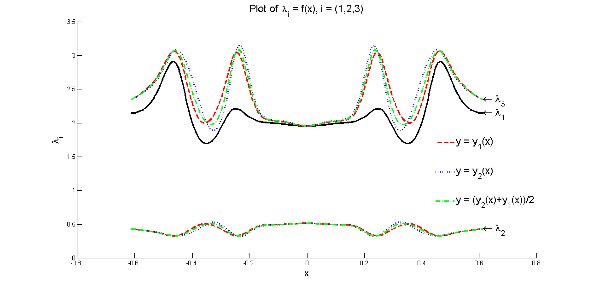
We plot the profile of the three eigenvalues $\lambda_{i}$ along the inner and outer boundaries $y_{1}$ and $y_{2}$ of the carpet, as well as along the curve located half way from these, i.e. $(y_{2}(x)+y_{1}(x))/2$. We can see in Fig. 1 that none of the eigenvalues vanish and they satisfy the inequality $0<\lambda_{2}\leq\lambda_{1}\leq\lambda_{3}$, a fact which can be also readily shown. We further note that $\lambda_{1}$ and $\lambda_{2}$ take values strictly within $1.5$ and $3.5$.

Thanks to the cylindrical geometry, the problem splits into $p$ and $s$ polarizations. In p polarization, we have:

in the carpet, where ${\bf H}_{l}=(H_{3}(x,y)-H_{3}^{i}(x,y)){\bf e}_{z}$ is the diffracted field parallel to the cylinder axis. Importantly, ${\bf H}_{l}$ satisfies the usual outgoing wave conditions as well as the Neumann data $\partial H_{3}/\partial n=\partial H_{3}^{i}/\partial n$ on the ground plane and the inner boundary of the cloak, with $H_{3}^{i}(x,y){\bf e}_{z}$ the incident field which is a beam generated by a constant field on a segment located at the upper left corner of the computational domain, and making an angle of $45$ degrees with the horizontal axis. Moreover, $\underline{\underline{\varepsilon^{\prime}_{T}}}$ is the upper left block diagonal part of $\underline{\underline{\varepsilon^{\prime}}}$ and $\mu^{\prime}_{33}$ the third diagonal entry of $\underline{\underline{\mu^{\prime}}}$, as deduced from (1) and (4).

Such an anisotropic permittivity $\underline{\underline{\varepsilon^{\prime}_{T}}}$ could be achieved e.g. using some thin wires of metal diluted in dielectrics [21, 22] to meet the condition that its eigenvalue $\lambda_{2}$ is lower than $1$, see Fig. 1. Moreover, $\mu^{\prime}_{33}=\lambda_{1}$ involves some artificial magnetism which would require some resonant elements such as split ring resonators [23] used in the design of the first invisibility cloak [3].

In what follows, we consider a plane wave and a beam incident from the top at the wavelength $\lambda=0.06$. In Fig. 2, we report some computations where the plane wave is coming from above and the beam is incident from the top left corner, making an angle of $\theta=45$ degrees with the normal to the ground plane. We note that the field diffracted by the flat ground plane with infinite conducting condition i.e. a mirror, cf. Fig. 2(d), and by an infinite conducting object i.e. a curved mirror surrounded by the carpet, cf. Fig. 2(c), indeed superimpose. Of course, the field diffracted by the curved mirror on its own, cf. Fig. 2(b), is much different.

We then repeat the same simulation with a Gaussian beam in order to further analyse the effect of the carpet in a more realistic physical situation. We report these computations in Fig. 3 where it should be noted that the beam reflected by the carpet appears to have a waist closer to that of the incident beam than in the case of a flat mirror. This might be attributed to the fact that the optical path followed by the center of the beam is smaller in the case of a carpet.

Let us finally consider the linear geometric transform:

where $z^{\prime}$ is a stretched vertical coordinate. It is easily seen that this linear geometric transform maps the arbitrary domain $D=\bigcup_{(u,v)\in{(0,1)}^{2}}\{(x(u,v),y(u,v))\}$ within the plane $xy$ onto the surface $z^{\prime}=z_{1}(x,y)$, and leaves the surface $z=z_{2}(x,y)$ unchanged. Importantly, there is a one-to-one correspondence between the domain $D$ and the surfaces $z^{\prime}=z_{1}$ and $z^{\prime}=z_{2}$. The surfaces $z_{1}$ and $z_{2}$ are assumed to be differentiable, and this ensures that the carpet won’t display any singularity on its inner boundary.

The linear transform (8) is expressed in a Cartesian basis as: ${\bf J}_{xx^{\prime}}=\left(\begin{array}[]{ccc}1&0&0\\ 0&1&0\\ \frac{\partial z}{\partial x^{\prime}}&\frac{\partial z}{\partial y^{\prime}}&\frac{1}{\alpha}\\ \end{array}\right)$ where $\alpha=(z_{2}-z_{1})/z_{2}$ and from the chain rule

This leads to the inverse symmetric tensor ${\bf T}^{-1}$ which is fully described by seven non vanishing entries in a Cartesian basis:

We note that the entries of the transformation matrix in (10) reduce to those of (4) when $\frac{\partial z}{\partial x^{\prime}}$ vanishes. The corresponding eigenvalues have the similar structure to (5) and are once again strictly positive and bounded, see Fig. 4, hence the material parameters are non-singular.

Let us now compute the total electromagnetic field for a plane wave normally incident upon a three-dimensional carpet. We have implemented the weak form of this scattering problem in the finite element package COMSOL using second order finite edge elements which behave nicely under geometric changes. Perfectly Matched Layers (PMLs), which can be seen as a stretch of coordinates, further enable us to model the unbounded domain. We choose the electric field ${\bf E}=(E_{1},E_{2},E_{3})(x,y,z)$ as the unknown in the Hilbert space $H({\rm curl},\Omega)=\{{\bf v}\in{[L^{2}(\Omega)]}^{3}\;,{\rm curl}{\bf v}\in{[L^{2}(\Omega)]}^{3}\}$ of curl-conforming fields [9], and therefore look for solutions of

where $k_{0}=\omega\sqrt{\mu_{0}\varepsilon_{0}}=\omega/c$ is the wavenumber, $c$ being the speed of light in vacuum, and $\underline{\underline{\varepsilon^{\prime}}}$ and $\underline{\underline{\mu^{\prime}}}$ are defined by Eqs. (1). Also, ${\bf E}={\bf E}_{i}+{\bf E}_{d}$, where ${\bf E}_{i}$ is the incident field (here a field approximating a plane wave incident from the top which is generated by a constant field on a flat surface on the upper part of the computational domain) and ${\bf E}_{d}$ is the diffracted field which decreases inside the PMLs. We note that we also used this setting to retrieve our former computations assuming an electric field with the form $(E_{1},E_{2},0)$ in (11) to take advantage of pull-back properties of edge-elements, leading again to Fig. 2 when we compute the curl of the numerical solution and plot the real part of the longitudinal component of $(0,0,H_{3})$

In this three-dimensional setting, we consider a plane wave incident from above at normal incidence: ${\bf E}_{i}=e^{-ikz}{\bf e}_{3}$, with wavenumber $k=2\pi/0.3$. The carpet has inner and outer surfaces given by:

where $\rho(\theta)=r(1-0.1\cos(5\theta))$ with $r=\sqrt{x^{2}+y^{2}}$ and $\theta=2\arctan(y/(x+\sqrt{x^{2}+y^{2}}))$ with $h_{1}=0.2$, $h_{2}=0.3$, $c_{1}=0.003$, $c_{1}=0.005$ $d_{1}=d_{2}=200$ and $\sigma=0.3$.

It is clearly seen from panels (c) and (d) in Fig. 5 that although of a complex non-convex shape, see (e), the carpet reflects the plane wave nearly like a flat ground plane would. When the bump is not covered by the carpet, the scattering is much worse, see (a) and (b).

Finally, we repeat these simulations for a Gaussian beam in oblique incidence (making an angle $\pi/4$ with the vertical axis). This requires a computational domain shaped as a prism, see Fig. 6. We note that the plots of the field are indeed symmetric with the $xOz$ plane in the case of a flat mirror, see Fig. 6(a-b), and a deformed mirror surrounded by the carpet, see Fig. 6(d-e). However, the diffraction by a deformed mirror is clearly giving rise to an asymmetric field, see Fig. 6(c).

In this paper, we have shown that it is possible to design two-dimensional and three-dimensional carpets of an arbitrary shape, using a similar approach to Fourier-based cloaks [24]. Such carpets do not exhibit any singular material parameters on their inner boundary, unlike invisibility cloaks, as they are based upon a one-to-one geometric transform. The next step towards the realization of such carpets might involve some structural elements such as conducting thin-straight wires and split ring resonators [23] to tune the permittivity and permeability to required values depending upon light polarization. The rapid experimental progress in the construction of carpets getting close to optical frequencies [25, 26, 27] suggests that our designs might soon come to life.

The authors acknowledge insightful discussions with A. Diatta, G. Demesy, M. Farhat, A. Nicolet and F. Zolla.

References

- [1] J.B. Pendry, D. Shurig, D.R. Smith, “Controlling electromagnetic fields,” Science 312, 1780-1782 (2006).
- [2] U. Leonhardt, “Optical conformal mapping,” Science 312 1777-1780 (2006).
- [3] D. Schurig et al., “Metamaterial electromagnetic cloak at microwave frequencies,” Science 314, 977-980 (2006).
- [4] R.V. Kohn and M. Vogelius, “Identification of an unknown conductivity by means of measurements at the boundary,” Inverse Problems D. McLaughin ed., SIAM-AMS Proc. 14 113-123 (1984)
- [5] A. Greenleaf, M. Lassas and G. Uhlmann, “On nonuniqueness for Calder�on�s inverse problem,”Math. Res. Lett. 10, 685-693 (2003).
- [6] N.A. Nicorovici, R.C. McPhedran and G.W. Milton,“Optical and dielectric properties of partially resonant composites,” Phys. Rev. B 49, 8479-8482 (1994).
- [7] A. Alu and N. Engheta, “Achieving transparency with plasmonic and metamaterial coatings,” Phys. Rev. E 72 016623 (2005).
- [8] A.J. Ward and J.B. Pendry, “Refraction and geometry in Maxwell’s equations,” J. Mod. Opt. 43, 773-793 (1996).
- [9] A. Nicolet et al. “Transformation methods in computational electromagnetism,” J. Appl. Phys. 75, 6036-6038 (1994).
- [10] E.G. Post, Formal Structure of Electromagnetics; General Covariance and Electromagnetics (Interscience, 1962).
- [11] U. Leonhardt and T. G. Philbin, “General relativity in electrical engineering,” New J. Phys. 8, 247 (2006).
- [12] F. Zolla, S. Guenneau, A. Nicolet and J.B. Pendry, “Electromagnetic analysis of cylindrical invisibility cloaks and the mirage effect”, Opt. Lett. 32, 1069-1071 (2007).
- [13] J.B. Pendry and S.A. Ramakrishna, “Focussing light using negative refraction,” J. Phys. Cond. Matter 15, 6345 (2003).
- [14] W. Cai, U.K. Chettiar, A.V. Kildiev and V.M. Shalaev, “Optical Cloaking with metamaterials”, Nature 1, 224-227 (2007).
- [15] M. Farhat, S. Guenneau, A.B. Movchan and S. Enoch, “Achieving invisibility over a finite range of frequencies,” Opt. Express 16, 5656-5661 (2008)
- [16] A. Greenleaf, Y. Kurylev, M. Lassas and G. Uhlmann, “Isotropic transformation optics: approximate acoustic and quantum cloaking,” New J. Physics 10, 115024 (2008)
- [17] P. Zhang, Y. Jin and S. He, “Obtaining a nonsingular two-dimensional cloak of complex shape from a perfect three-dimensional cloak,” Appl. Phys. Lett. 93, 243502 (2008)
- [18] W.X. Jiang et al. “Invisibility cloak without singularity,” Appl. Phys. Lett. 93, 194102 (2008).
- [19] U. Leonhardt and T. Tyc, “Broadband invisibility by non-euclidean cloaking,” Science 323, 110 (2009).
- [20] J. Li and J.B. Pendry, “Hiding under the carpet: a new strategy for cloaking,” Phys. Rev. Lett. 101, 203901 (2008).
- [21] J.B. Pendry, A.J. Holden, W.J. Stewart and I. Youngs,“ Extremely low frequency plasmons in metallic mesostructures” Phys. Rev. Lett. 76, 4773 (1996)
- [22] S. Enoch, G. Tayeb, P. Sabouroux, N. Guerin and P. Vincent, “A metamaterial for directive emission,” Phys. Rev. Lett. 89, 213902 (2002).
- [23] J.B. Pendry, A.J. Holden, W.J. Stewart and I. Youngs, “Magnetism from conductors and enhanced nonlinear phenomena” IEEE Trans. Micr. Theo. Tech. 47, 2075 (1999).
- [24] A. Nicolet, F. Zolla and S. Guenneau, “Electromagnetic analysis of cylindrical cloaks of an arbitrary cross section.” Opt. Lett. 33, 1584-1586 (2008).
- [25] R. Liu, C. Ji, J.J. Mock, J.Y. Chin, T.J. Cui and D.R. Smith, “Broadband Ground-Plane Cloak,” Science 323, 366 (2008).
- [26] J. Valentine, J. Li, T. Zentgraf, G. Bartal and X. Zhang, “An optical cloak made of dielectrics.” Nature Mater. 8, 569 (2009).
- [27] L.H. Gabrielli, J. Cardenas, C.B. Poitras and M. Lipson, “Silicon nanostructure cloak operating at optical frequencies,” Nature Photonics (2009). Doi:10.1038/nphoton.2009.117