A survey of Magnus representations for mapping class groups and homology cobordisms of surfaces

Takuya Sakasai ^†^†thanks: Work partially supported by Grant-in-Aid for Scientific Research, (No.˜21740044), Ministry of Education, Science, Sports and Technology, Japan. Address: Department of Mathematics, Tokyo Institute of Technology,
2-12-1 Oh-okayama, Meguro-ku, Tokyo, 152-8551, Japan.
email: sakasai@math.titech.ac.jp

Abstract

This is a survey of Magnus representations with particular emphasis on their applications to mapping class groups and monoids (groups) of homology cobordisms of surfaces. In the first half, we begin by recalling the basics of the Fox calculus and overview Magnus representations for automorphism groups of free groups and mapping class groups of surfaces with related topics. In the latter half, we discuss in detail how the theory in the first half extends to homology cobordisms of surfaces and present a number of applications from recent researches.

keywords

Magnus representation, Fox calculus, mapping class group, acyclic closure, homology cylinder, homology cobordism.

Classification:

7M05, 57N70, 20F14, 20F34, 57M27, 20C07.

1 Introduction

Let $\Sigma_{g,n}$ be a compact connected oriented smooth surface of genus $g$ with $n$ boundary components ( $n$ may be $0$ ). We take a base point $p$ in $\partial\Sigma_{g,n}$ when $n\geq 1$ and arbitrarily when $n=0$ . The mapping class group $\mathcal{M}_{g,n}$ of $\Sigma_{g,n}$ is defined as the group of all isotopy classes of orientation-preserving diffeomorphisms of $\Sigma_{g,n}$ which fix the boundary pointwise. The area of research covered by the mapping class group in contemporary mathematics is very broad: algebraic geometry, differential geometry, hyperbolic geometry, complex analysis, topology, combinatorial group theory, mathematical physics etc. The group $\mathcal{M}_{g,n}$ serves as the modular group of the Teichmüller space, which is the main theme of this handbook, and this yields a strong connection among the above subjects.

Now let us consider $\mathcal{M}_{g,n}$ from a topological point of view, which is our approach for studying $\mathcal{M}_{g,n}$ in this chapter. While $\mathcal{M}_{g,n}$ does not act on the surface $\Sigma_{g,n}$ itself, it works as transformation groups of many discretized objects related to $\Sigma_{g,n}$ : the set of isotopy classes of curves, the fundamental group $\pi_{1}(\Sigma_{g,n},p)$ (when $n\geq 1$ ), the homology groups etc. In many cases, these discretized (simplified in a sense) data lose no topological information on the objects involved, for the classical theory of surface topology says that homotopical information of a surface governs its topology. For example, we use $\mathcal{M}_{g,n}$ more often than the diffeomorphism group of $\Sigma_{g,n}$ in the construction of three-dimensional manifolds by Heegaard splittings or Dehn surgery, and also that of surface bundles over a manifold. When $n=1$ , a theorem of Dehn and Nielsen says that an element in $\mathcal{M}_{g,1}$ is completely characterized by its action on $\pi_{1}(\Sigma_{g,1},p)$ , which is a free group of rank $2g$ . This suggests a method for studying $\mathcal{M}_{g,n}$ through the theory of the automorphism group of a free group.

Magnus representations are matrix representations for free groups and their automorphism groups. The definition is usually given in terms of the Fox derivative and it looks like a Jacobian matrix of a differentiable map. With their relationship to homology and cohomology of groups, Magnus representations have been used as a fundamental tool for studying various groups by researchers in combinatorial group theory for many years. En route, applications to $\mathcal{M}_{g,n}$ have also been given.

Compared with the history of mapping class groups and automorphism groups of free groups, the study of monoids and groups of homology cobordisms over a surface is a quite new theme of research. This research was independently initiated by Goussarov [43] and Habiro [48] in their investigations of three-dimensional manifolds via so-called clover or clasper surgery, which are known to be essentially the same. These surgery techniques are said to be a “topological commutator calculus”, which invokes a connection to $\mathcal{M}_{g,n}$ as automorphisms of $\pi_{1}(\Sigma_{g,n},p)$ . In fact, Garoufalidis-Levine [35] established a connection between the above surgery techniques and classical algebraic topology related to $\mathcal{M}_{g,n}$ in terms of Massey products on the first cohomology of three-dimensional manifolds.

In this chapter, we use the word “homology cylinders” for homology cobordisms over a surface with fixed markings of their boundaries. These markings are necessary to define a product operation on the set of homology cylinders as a generalization of the mapping class group. We can consider, for example, homology 3-spheres and pure string links with $n$ strings to be homology cylinders over $\Sigma_{0,1}$ and $\Sigma_{0,n+1}$ . For a given homology cylinder over $\Sigma_{g,n}$ , we can construct another one by changing its markings by using $\mathcal{M}_{g,n}$ . Therefore homology cylinders enable us to treat important objects in three-dimensional topology simultaneously. This motivates the study of homology cylinders with particular stress on its algebraic structure.

The purpose of this chapter is to survey research on structures of mapping class groups and monoids (groups) of homology cylinders through their Magnus representations as a common tool for study. Note that homology cylinders are also discussed in the chapter of Habiro and Massuyeau [49]. However, our approach here is distinct from theirs and more group-theoretical. The author hopes that their chapter and the present one could complement each other and offer the readers an introduction to this fruitful subject.

Here we briefly mention the content of this chapter. Basically, it is divided into two parts: The first part is intended for serving as a survey of Magnus representations for automorphism groups of free groups and mapping class groups of surfaces. In Section 2, we first recall the Fox calculus as a tool for many computations in this chapter. We put stress on its relationship to homology and cohomology of groups. Section 3 is devoted to give a machinery of Magnus representations with relations to automorphisms of the derived quotients of a free group. Finally, in Section 4, we overview applications of Magnus representations to mapping class groups of surfaces following works of Morita and Suzuki. The second part of this chapter begins in Section 5, where the monoid and related groups of homology cylinders over a surface are introduced. Sections 6 and 7 are devoted to discussing methods for extending Magnus representations for mapping class groups to homology cylinders. In Section 8, we present several topics on homology cylinders where Magnus representations play important roles.

Convention.

All maps act on elements from the left. We often use the same notation to write a map and induced maps on quotients of its source or target. Homology and cohomology groups are assumed to be with coefficients in the ring of integers $\mathbb{Z}$ and all manifolds are assumed to be smooth unless otherwise indicated.

The author is deeply grateful to Athanase Papadopoulos for giving him a chance to write this chapter and providing many valuable suggestions. The author also would like to thank Kazuo Habiro, Nariya Kawazumi, Teruaki Kitano, Gwénaël Massuyeau, Takayuki Morifuji, Takao Satoh and Masaaki Suzuki for their careful reading and helpful comments on the manuscript, and Hiroshi Goda for permitting the author to use the pictures in Example 8.3.

2 Fox calculus

We begin by recalling the Fox calculus, which was defined by Fox in the 1950s and which has been known as an important tool in the study of free groups and their automorphisms. Magnus representations are defined as an application of this machinery. Historically, Magnus representations were defined without the Fox calculus. However, we use the Fox calculus since it is now widely accepted to be standard and offers a clear connection to low-dimensional topology. Good references for this topic have been the original paper of Fox [32] and Birman’s book [14]. Our discussion is almost parallel to the latter with particular stress on the relationship of the Fox calculus to homology and cohomology of groups. The relation becomes a key to generalizing the machinery so that it can be applied to objects in more broad range than free groups and their automorphisms in the latter half of this chapter.

Since we shall work in non-commutative rings almost everywhere in this chapter, we first need to fix our notation in detail.

Notation.

For a group $G$ and two of its subgroups $G_{1}$ and $G_{2}$ , we denote by $[G_{1},G_{2}]$ the commutator subgroup of $G_{1}$ and $G_{2}$ . We set $[x,y]=xyx^{-1}y^{-1}$ for $x$ , $y\in G$ . The integral (or rational) group ring of $G$ is denoted by $\mathbb{Z}[G]$ (or $\mathbb{Q}[G]$ ). For a matrix $A$ with entries in a ring $R$ and a ring homomorphism $\varphi:R\to R^{\prime}$ , we denote by ${}^{\varphi}A$ the matrix obtained from $A$ by applying $\varphi$ to each entry. $A^{T}$ denotes the transpose of $A$ . When $R$ is $\mathbb{Z}[G]$ or its right field of fractions (if it exists), we denote by $\overline{A}$ the matrix obtained from $A$ by applying the involution induced from $(x\mapsto x^{-1},\ x\in G)$ to each entry. For a module $M$ , we write $M^{n}$ the module of column vectors with $n$ entries in $M$ .

2.1 Fox derivatives

Let $G$ be a group and let $M$ be a left $\mathbb{Z}[G]$ -module. A crossed homomorphism (or derivation) from $G$ to $M$ is a map $f:G\to M$ satisfying

f(xy)=f(x)+xf(y)

for all $x,y\in G$ . In other words, it is a homomorphism $(f,\mathrm{id}_{G}):G\to M\rtimes G$ , where $M\rtimes G$ is the semi-direct product with the group structure given by

(m_{1},g_{1})\cdot(m_{2},g_{2})=(m_{1}+g_{1}m_{2},g_{1}g_{2})

for $m_{1},m_{2}\in M$ and $g_{1},g_{2}\in G$ . When $G$ is $F_{n}$ , a free group of rank $n$ , the latter description shows that a crossed homomorphism $f:F_{n}\to M$ is determined by its values on any generating set of $F_{n}$ . In general, if $G$ has a (not necessarily finite) presentation $\langle x_{1},x_{2},\ldots\mid r_{1},r_{2},\ldots\rangle$ , crossed homomorphisms $f:G\to M$ correspond to crossed homomorphisms $f:\langle x_{1},x_{2},\ldots\rangle\to M$ satisfying $f(r_{i})=0$ for all $i=1,2,\ldots$ , where $\langle x_{1},x_{2},\ldots\rangle$ is the free group generated by $\{x_{1},x_{2},\ldots\}$ .

Let us define Fox derivatives for $F_{n}$ . We take a basis $\{\gamma_{1},\gamma_{2},\ldots,\gamma_{n}\}$ of $F_{n}$ . The group $F_{n}$ acts on $\mathbb{Z}[F_{n}]$ by left multiplication, so that $\mathbb{Z}[F_{n}]$ is a left $\mathbb{Z}[F_{n}]$ -module.

Definition 2.1.

The Fox derivative (or free derivative) with respect to $\gamma_{j}$ in the basis $\{\gamma_{1},\gamma_{2},\ldots,\gamma_{n}\}$ is the crossed homomorphism

\frac{\partial}{\partial\gamma_{j}}:F_{n}\longrightarrow\mathbb{Z}[F_{n}]

defined by $\displaystyle\frac{\partial\gamma_{i}}{\partial\gamma_{j}}=\delta_{ij}$ (Kronecker’s delta). We use the same notation for its extension

\frac{\partial}{\partial\gamma_{j}}:\mathbb{Z}[F_{n}]\longrightarrow\mathbb{Z}[F_{n}]

to $\mathbb{Z}[F_{n}]$ as an additive map.

Fundamental properties of Fox derivatives are as follows. Let $\mathfrak{t}:\mathbb{Z}[F_{n}]\to\mathbb{Z}$ be the trivializer (or augmentation homomorphism) defined by $\mathfrak{t}(\sum_{v\in F_{n}}a_{v}v)=\sum_{v\in F_{n}}a_{v}$ .

Proposition 2.2.

$(1)$ The equality $\displaystyle\frac{\partial\gamma_{i}^{-1}}{\partial\gamma_{j}}=-\delta_{ij}\gamma_{i}^{-1}$ holds.

$(2)$ For $g,h\in\mathbb{Z}[F_{n}]$ , we have

\displaystyle\frac{\partial(gh)}{\partial\gamma_{j}}=\frac{\partial g}{\partial\gamma_{j}}\mathfrak{t}(h)+g\frac{\partial h}{\partial\gamma_{j}}.

$(3)$ $($ Chain rule $)$ Let $\varphi:F_{n}\to F_{n}$ be an endomorphism of $F_{n}$ . For any $w\in F_{n}$ , we have

\frac{\partial\varphi(w)}{\partial\gamma_{j}}=\sum_{k=1}^{n}\left(\varphi\left(\frac{\partial w}{\partial\gamma_{k}}\right)\right)\left(\frac{\partial\varphi(\gamma_{k})}{\partial\gamma_{j}}\right).

$(4)$ $($ “Fundamental formula” of Fox calculus $)$ For $g\in\mathbb{Z}[F_{n}]$ , we have

g-\mathfrak{t}(g)=\sum_{j=1}^{n}\frac{\partial g}{\partial\gamma_{j}}(\gamma_{j}-1).

$(5)$ Let $\rho:F_{n}\to\Gamma$ be a homomorphism. Then $v\in F_{n}$ satisfies

\rho\left(\frac{\partial v}{\partial\gamma_{j}}\right)=0\qquad\mbox{for $j=1,2,\ldots,n$}

if and only if $v\in[\mathop{\mathrm{Ker}}\nolimits\rho,\mathop{\mathrm{Ker}}\nolimits\rho]$ .

(1) and (2) are easily proved. As for (3), (4) and (5), we prove them in the next subsections by relating them to homology and cohomology of groups.

2.2 The Magnus representation for a free group

Now we define the Magnus representation for $F_{n}$ by using Fox derivatives. Let $S=\{s_{1},s_{2},\ldots,s_{n}\}$ be a set of formal parameters. We denote by $(\mathbb{Z}[F_{n}])[S]$ the polynomial ring over $\mathbb{Z}[F_{n}]$ with variables $S$ , where the elements of $S$ are supposed to commute with one another and with the elements of $\mathbb{Z}[F_{n}]$ .

Definition 2.3.

For $w\in F_{n}$ , we put a matrix

(w):=\begin{pmatrix}w&\displaystyle\sum_{j=1}^{n}\left(\frac{\partial w}{\partial\gamma_{j}}\right)s_{j}\\ 0&1\end{pmatrix}.

Then the map $w\mapsto(w)$ gives a homomorphism $F_{n}\to\mathrm{GL}(2,(\mathbb{Z}F_{n})[S])$ called the Magnus representation for $F_{n}$ .

This representation was first given by Magnus [77] without using Fox derivatives (see Remark 2.4). It is clearly injective. On the other hand, it follows from Proposition 2.2 (5) that for a homomorphism $\rho:F_{n}\to\Gamma$ , the kernel of the homomorphism $w\mapsto{}^{\rho}(w)$ is $[\mathop{\mathrm{Ker}}\nolimits\rho,\mathop{\mathrm{Ker}}\nolimits\rho]$ . In particular, if we take the abelianization map $\mathfrak{a}:F_{n}\to H_{1}:=H_{1}(F_{n})\cong\mathbb{Z}^{n}$ as $\rho$ , we obtain an injection of the metabelian quotient $F_{n}/[[F_{n},F_{n}],[F_{n},F_{n}]]$ into $\mathrm{GL}(2,(\mathbb{Z}[H_{1}])[S])$ , where the definition of $(\mathbb{Z}[H_{1}])[S]$ is given by replacing $F_{n}$ with $H_{1}$ in the definition of $(\mathbb{Z}[F_{n}])[S]$ .

Remark 2.4.

The Magnus representation of $F_{n}$ can be described by using crossed homomorphisms. Indeed, we can unify the Fox derivatives $\displaystyle\frac{\partial}{\partial\gamma_{j}}$ $(j=1,2,\ldots,n)$ into a homomorphism

\left(\left(\frac{\partial}{\partial\gamma_{1}},\frac{\partial}{\partial\gamma_{2}},\ldots,\frac{\partial}{\partial\gamma_{n}}\right)^{T},\mathrm{id}_{F_{n}}\right):F_{n}\longrightarrow(\mathbb{Z}[F_{n}])^{n}\rtimes F_{n}.

This map is equivalent to the Magnus representation. On the other hand, if we consider a homomorphism $F_{n}\to(\mathbb{Z}[F_{n}])^{n}\rtimes F_{n}$ given by

\gamma_{j}\longmapsto\bordermatrix{&j\ \ \,&\cr&(0,\ldots,0,\,1\,,0,\ldots,0)^{T},&\gamma_{j}},

we can define the Fox derivatives as its first projection. This corresponds to Magnus’ original description.

2.3 Homology and cohomology of groups

In this subsection, we interpret the definition and fundamental properties of Fox derivatives and the Magnus representation for $F_{n}$ in terms of homology and cohomology. This interpretation makes it easier to give their topological applications. As space is limited, however, we refer to Brown’s book [16] for the general theory. Instead, here we give explicit chain and cochain complexes to calculate the homology and cohomology of a given group.

Let $G$ be a group and $M$ be a left $\mathbb{Z}[G]$ -module. We denote by $C_{i}$ the free $\mathbb{Z}[G]$ -module generated by the symbols $[g_{1}|g_{2}|\cdots|g_{i}]$ corresponding to $i$ -tuples of elements $g_{1},g_{2},\ldots,g_{i}$ of $G$ ( $C_{0}\cong\mathbb{Z}[G]$ generated by $[\cdot]$ ). We define the chain complex $C_{\ast}(G;M)$ and cochain complex $C^{\ast}(G;M)$ by

	$\displaystyle C_{i}(G;M)$	$\displaystyle=C_{i}\otimes_{\mathbb{Z}[G]}M,$
	$\displaystyle C^{i}(G;M)$	$\displaystyle=\operatorname{Hom}_{\mathbb{Z}[G]}(C_{i},M).$

Here the tensor product is taken for the right $\mathbb{Z}[G]$ -module $C_{i}$ and the left $\mathbb{Z}[G]$ -module $M$ , and $\operatorname{Hom}_{\mathbb{Z}[G]}(C_{i},M)$ consists of $\mathbb{Z}[G]$ -“equivariant” homomorphisms $f$ in the sense that $f$ satisfies $f(cg)=g^{-1}f(c)$ for $c\in C_{i}$ and $g\in G$ . (These conventions are slightly different from those in [16].) The boundary operator $\partial_{i}:C_{i}(G;M)\to C_{i-1}(G;M)$ is given by

		$\displaystyle\ \ \partial_{i}([g_{1}\|g_{2}\|\cdots\|g_{i}]\otimes m)$
	$\displaystyle=$	$\displaystyle\ [g_{2}\|g_{3}\|\cdots\|g_{i}]\otimes g_{1}^{-1}m-[g_{1}g_{2}\|g_{3}\|\cdots\|g_{i}]\otimes m$
		$\displaystyle+[g_{1}\|g_{2}g_{3}\|g_{4}\|\cdots\|g_{i}]-\cdots+(-1)^{i-1}[g_{1}\|\cdots\|g_{i-2}\|g_{i-1}g_{i}]\otimes m$
		$\displaystyle+(-1)^{i}[g_{1}\|\cdots\|g_{i-2}\|g_{i-1}]\otimes m$

and the coboundary operator $\delta_{i}:C^{i}(G;M)\to C^{i+1}(G;M)$ is given by

		$\displaystyle\ \ (\delta_{i}f)([g_{1}\|g_{2}\|\cdots\|g_{i+1}])$
	$\displaystyle=$	$\displaystyle\ g_{1}f([g_{2}\|g_{3}\|\cdots\|g_{i+1}])-f([g_{1}g_{2}\|g_{3}\|\cdots\|g_{i+1}])$
		$\displaystyle+f([g_{1}\|g_{2}g_{3}\|g_{4}\|\cdots\|g_{i+1}])-\cdots+(-1)^{i}f([g_{1}\|\cdots\|g_{i-1}\|g_{i}g_{i+1}])$
		$\displaystyle+(-1)^{i+1}f([g_{1}\|\cdots\|g_{i-1}\|g_{i}])$

for $f\in C^{i}(G;M)$ regarded as a function from the set of symbols $[g_{1}|g_{2}|\cdots|g_{i}]$ to $M$ . We denote the corresponding homology and cohomology groups by $H_{\ast}(G;M)$ and $H^{\ast}(G;M)$ . We obtain the following explicit description of homology and cohomology in degree $0$ by observing the complexes.

	$\displaystyle H_{0}(G;M)$	$\displaystyle=M/\langle m-gm\mid m\in M,g\in G\rangle,$
	$\displaystyle H^{0}(G;M)$	$\displaystyle=\{m\in M\mid\mbox{$gm=m$ for any $g\in G$}\}.$

Next we take a close look at $H^{1}(G;M)$ . The condition for $f\in C^{1}(G;M)$ to be a cocycle is that

0=(\delta_{1}f)([g_{1}|g_{2}])=g_{1}f([g_{2}])-f([g_{1}g_{2}])+f([g_{1}])

holds for any $g_{1},g_{2}\in G$ . If we naturally identify a cochain in $C^{1}(G;M)$ with a map from $G$ to $M$ , this cocycle condition is nothing more than the definition of crossed homomorphisms from $G$ to $M$ mentioned in Section 2.1. Therefore the module of $1$ -cocycles is written as the module $\mathrm{Cross}(G;M)$ of crossed homomorphisms from $G$ to $M$ . A $1$ -coboundary is obtained from each element $m\in M\cong C^{0}(G;M)$ corresponding to the function $[\cdot]\mapsto m$ , and we have

(\delta_{0}m)([g])=gm-m

for $m\in M$ and $g\in G$ . We call such a crossed homomorphism (after the above identification) a principal crossed homomorphism and denote the module of principal crossed homomorphisms by $\mathrm{Prin}(G;M)$ . Consequently we have

H^{1}(G;M)\cong\mathrm{Cross}(G;M)/\mathrm{Prin}(G;M).

Example 2.5.

Let $M=\mathbb{Z}$ with the trivial $G$ -action. We have

	$\displaystyle H_{0}(G;\mathbb{Z})$	$\displaystyle\cong H^{0}(G;\mathbb{Z})\cong\mathbb{Z},$
	$\displaystyle H_{1}(G;\mathbb{Z})$	$\displaystyle\cong G/[G,G],\ \mbox{the abelianization of $G$},$
	$\displaystyle H^{1}(G;\mathbb{Z})$	$\displaystyle\cong\operatorname{Hom}(G,\mathbb{Z})=\operatorname{Hom}(H_{1}(G;\mathbb{Z}),\mathbb{Z}).$

Remark 2.6.

For any $\mathbb{Z}[G]$ -bimodule $M$ (for example, $M=\mathbb{Z}[G]$ ), $C_{\ast}(G;M)$ and $C^{\ast}(G;M)$ have natural right actions of $G$ , with our convention. Moreover, the operators $\partial_{i}$ and $\delta_{i}$ are equivariant with respect to this right action, so that $H_{\ast}(G;M)$ and $H^{\ast}(G;M)$ become right $\mathbb{Z}[G]$ -modules.

Let us return to our concern. The Fox derivative $\displaystyle\frac{\partial}{\partial\gamma_{j}}$ can be seen as a $1$ -cocycle in $\mathrm{Cross}(F_{n};\mathbb{Z}[F_{n}])\subset C^{1}(F_{n};\mathbb{Z}[F_{n}])$ sending $\gamma_{j}$ to $1$ and $\gamma_{i}$ $(i\neq j)$ to $0$ . Since a crossed homomorphism $F_{n}\to\mathbb{Z}[F_{n}]$ is determined by its values on any basis of $F_{n}$ , we see that $\left\{\displaystyle\frac{\partial}{\partial\gamma_{1}},\displaystyle\frac{\partial}{\partial\gamma_{2}},\ldots,\displaystyle\frac{\partial}{\partial\gamma_{n}}\right\}$ forms a basis of $\mathrm{Cross}(F_{n};\mathbb{Z}[F_{n}])$ as a right $\mathbb{Z}[F_{n}]$ -module.

Proof of Proposition $\ref{prop:foxproperty}(3)$ .

Let $\varphi^{\ast}\mathbb{Z}[F_{n}]$ be the left $\mathbb{Z}[F_{n}]$ -module whose underlying abelian group is $\mathbb{Z}[F_{n}]$ but on which $F_{n}$ acts through $\varphi$ . We easily see that $\mathrm{Cross}(F_{n};\varphi^{\ast}\mathbb{Z}[F_{n}])$ is a free right $\mathbb{Z}[F_{n}]$ -module of rank $n$ generated by

\left\{\varphi\left(\displaystyle\frac{\partial}{\partial\gamma_{1}}\right),\ \varphi\left(\displaystyle\frac{\partial}{\partial\gamma_{2}}\right),\ \ldots,\ \varphi\left(\displaystyle\frac{\partial}{\partial\gamma_{n}}\right)\right\},

where $F_{n}$ acts from the right by the usual, not through $\varphi$ , multiplication. Now the map $w\mapsto\displaystyle\frac{\partial\varphi(w)}{\partial\gamma_{j}}$ is in $\mathrm{Cross}(F_{n};\varphi^{\ast}\mathbb{Z}[F_{n}])$ , so that we can put $\displaystyle\frac{\partial\varphi(\cdot)}{\partial\gamma_{j}}=\displaystyle\sum_{k=1}^{n}\left(\varphi\left(\displaystyle\frac{\partial}{\partial\gamma_{k}}\right)\right)\cdot g_{k}$ . If we substitute $\gamma_{k}$ in this equality, we have $g_{k}=\displaystyle\frac{\partial\varphi(\gamma_{k})}{\partial\gamma_{j}}$ and our claim follows. ∎

Proof of Proposition $\ref{prop:foxproperty}(4)$ .

It suffices to show our claim when $g=v\in F_{n}$ , a monomial. We can easily check that the equality

\delta_{0}1=\sum_{j=1}^{n}\left(\frac{\partial}{\partial\gamma_{j}}\right)\cdot(\gamma_{j}-1)\quad\in C^{1}(F_{n};\mathbb{Z}[F_{n}])

holds for $1\in C^{0}(F_{n};\mathbb{Z}[F_{n}])\cong\mathbb{Z}[F_{n}]$ . Applying this $1$ -cochain to $v$ , we obtain the desired equality. ∎

Remark 2.7.

For groups $H\subset G$ and a left $\mathbb{Z}[G]$ -module $M$ , the relative homology $H_{\ast}(G,H;M)$ (resp. cohomology $H^{\ast}(G,H;M)$ ) can be defined by considering $C_{\ast}(G;M)/C_{\ast}(H;M)$ (resp. $\mathop{\mathrm{Ker}}\nolimits(C^{\ast}(G;M)\to C^{\ast}(H;M))$ ) as usual.

2.4 Fox derivatives in low-dimensional topology

Fox derivatives and low-dimensional topology are connected by using the topological definition of (co)homology of groups.

Convention.

For a connected CW-complex $X$ , we denote by $\widetilde{X}$ its universal covering. We take a base point $p$ of $X$ and a lift $\widetilde{p}$ of $p$ as a base point of $\widetilde{X}$ . The group $G:=\pi_{1}(X,p)$ acts on $\widetilde{X}$ from the right through its deck transformation group, namely, the lift of $\gamma\in G$ starting from $\widetilde{p}$ reaches $\widetilde{p}\gamma^{-1}$ . When $X$ is a finite complex, we regard the cellular chain complex $C_{\ast}(\widetilde{X})$ of $\widetilde{X}$ , on which $G$ acts from the right, as a collection of free right $\mathbb{Z}[G]$ -modules consisting of column vectors together with boundary operators given by left multiplication of matrices. For a left $\mathbb{Z}[G]$ -module $M$ , the twisted chain complex $C_{\ast}(X;M)$ is given by the tensor product of the right $\mathbb{Z}[G]$ -module $C_{\ast}(\widetilde{X})$ and the left $\mathbb{Z}[G]$ -module $M$ . This complex gives the twisted homology group $H_{\ast}(X;M)$ . The twisted cochain complex $C^{\ast}(X;M)$ and the twisted cohomology group $H^{\ast}(X;M)$ are defined similarly.

In topology, the homology $H_{\ast}(G;M)$ and cohomology $H^{\ast}(G;M)$ of a group $G$ with coefficients in a left $\mathbb{Z}[G]$ -module $M$ are defined as twisted (co)homology groups

	$\displaystyle H_{\ast}(G;M)$	$\displaystyle=H_{\ast}(K(G,1);M),$
	$\displaystyle H^{\ast}(G;M)$	$\displaystyle=H^{\ast}(K(G,1);M),$

where $K(G,1)$ is the Eilenberg-MacLane space of $G$ . The space $K(G,1)$ is characterized uniquely up to homotopy equivalence as a connected CW-complex satisfying

\pi_{1}(K(G,1))=G,\qquad\pi_{i}(K(G,1))=0\quad(i\geq 2).

Remark 2.8.

There are several methods for checking that this definition coincides with that in the previous section. We refer to Brown’s book [16] again. One method is to see that the complex in the previous section is derived from the fat realization of a (semi-)simplicial structure of $K(G,1)$ .

Note that for any CW-complex $X$ with $\pi_{1}X=G$ , we have

		$\displaystyle H_{0}(X;M)\cong H_{0}(G;M),\qquad H_{1}(X;M)\cong H_{1}(G;M),$
		$\displaystyle H^{0}(X;M)\cong H^{0}(G;M),\qquad H^{1}(X;M)\cong H^{1}(G;M)$

since $K(G,1)$ can be obtained from $X$ by attaching $3$ -cells, $4$ -cells, $\ldots$ , so that all higher homotopy groups are eliminated. We also see that there exists an epimorphism

(2.1)

The kernel is exactly the image of the Hurewicz homomorphism $\pi_{2}X\to H_{2}(X)$ .

For a group $G$ with a presentation $\langle x_{1},x_{2},\ldots\mid r_{1},r_{2},\ldots\rangle$ , we construct a $2$ -complex $X$ consisting of one $0$ -cell, say $p$ , one $1$ -cell for each generator and one $2$ -cell for each relation with an attaching map according to the word. Then $\pi_{1}X=G$ . Using this construction, we now look for a practical method for calculating $H_{1}(G;M)$ in case $G$ has a finite presentation $\langle x_{1},x_{2},\ldots,x_{k}\mid r_{1},r_{2},\ldots,r_{l}\rangle$ . Consider the chain complex

C_{2}(X;M)\stackrel{{\scriptstyle\partial_{2}}}{{\longrightarrow}}C_{1}(X;M)\stackrel{{\scriptstyle\partial_{1}}}{{\longrightarrow}}C_{0}(X;M)\longrightarrow 0.

This complex can be rewritten as

M^{l}\xrightarrow{D_{2}\cdot}M^{k}\xrightarrow{D_{1}\cdot}M\longrightarrow 0

with matrices $D_{1}$ , $D_{2}$ . Observing the lifts of the loops $x_{1},\ldots,x_{k}$ and $r_{1},\ldots r_{l}$ starting from the base point $\widetilde{p}$ of $\widetilde{X}$ , we see that

	$\displaystyle D_{1}$	$\displaystyle=\begin{pmatrix}x_{1}^{-1}-1&x_{2}^{-1}-1&\cdots&x_{k}^{-1}-1\end{pmatrix},$
	$\displaystyle D_{2}$	$\displaystyle=\left(\overline{\left(\frac{\partial r_{j}}{\partial x_{i}}\right)}\right)_{\begin{subarray}{c}{}1\leq i\leq k\\ 1\leq j\leq l\end{subarray}}$

over $\mathbb{Z}[G]$ . Here and hereafter the words “over $\mathbb{Z}[G]$ ” means that we are considering all entries to be in $\mathbb{Z}[G]$ as images of the natural homomorphism $\mathbb{Z}[\langle x_{1},\ldots,x_{k}\rangle]\to\mathbb{Z}[G]$ . The relation $D_{1}D_{2}=O$ follows from Proposition 2.2 (4). From this expression of $D_{2}$ , we actually see that Fox derivatives contribute to low-dimensional topology in the calculation of $H_{1}(G;M)=H_{1}(X;M)$ .

Example 2.9.

Let $\rho:G\to\Gamma$ be an epimorphism. Take a CW-complex $X$ with $\pi_{1}X=G$ . Then $C_{\ast}(X;\mathbb{Z}[\Gamma])$ just corresponds to the cellular complex of the $\Gamma$ -covering $X_{\Gamma}$ of $X$ with respect to $\rho$ . Hence we have

H_{1}(G;\mathbb{Z}[\Gamma])\cong H_{1}(X;\mathbb{Z}[\Gamma])\cong H_{1}(X_{\Gamma})\cong H_{1}(\mathop{\mathrm{Ker}}\nolimits\rho).

Proof of Proposition $\ref{prop:foxproperty}(5)$ .

First, we may suppose that $\rho:F_{n}\to\Gamma$ is an epimorphism. We now consider $H_{1}(F_{n};\mathbb{Z}[\Gamma])$ . The space $K(F_{n},1)$ is given by a bouquet $X$ of $n$ circles corresponding to the generating system $\{\gamma_{1},\gamma_{2},\ldots,\gamma_{n}\}$ of $F_{n}$ . By an observation similar to the one for the matrix $D_{2}$ above, we see that the abelianization map

\mathop{\mathrm{Ker}}\nolimits\rho\cong\pi_{1}X_{\Gamma}\longrightarrow H_{1}(X_{\Gamma})=\mbox{\lx@text@lbrace$1$-cycles on $X_{\Gamma}$\lx@text@rbrace}\subset C_{1}(X_{\Gamma})\cong(\mathbb{Z}[\Gamma])^{n}

is given by

v\longmapsto\sideset{{}^{\rho}\!}{{}^{T}}{\mathop{\left({\begin{array}[]{cccc}\overline{\displaystyle\frac{\partial v}{\partial\gamma_{1}}}&\overline{\displaystyle\frac{\partial v}{\partial\gamma_{2}}}&\cdots&\overline{\displaystyle\frac{\partial v}{\partial\gamma_{n}}}\end{array}}\right)}\nolimits}.

The kernel of this map is $[\mathop{\mathrm{Ker}}\nolimits\rho,\mathop{\mathrm{Ker}}\nolimits\rho]$ and our claim immediately follows. ∎

Example 2.10.

Let $X$ be the bouquet in the above proof of Proposition 2.2 (5) with base point $p$ . Consider the homology exact sequence

	$\displaystyle H_{1}(X;\mathbb{Z}[F_{n}])$	$\displaystyle\longrightarrow H_{1}(X,\{p\};\mathbb{Z}[F_{n}])\longrightarrow H_{0}(\{p\};\mathbb{Z}[F_{n}])$
		$\displaystyle\longrightarrow H_{0}(X;\mathbb{Z}[F_{n}])\longrightarrow H_{0}(X,\{p\};\mathbb{Z}[F_{n}]),$

which can be regarded as that for the pair $(F_{n},\{1\})$ of groups. Clearly $H_{1}(X;\mathbb{Z}[F_{n}])=H_{1}(\widetilde{X})=0$ and $H_{0}(X;\mathbb{Z}[F_{n}])=H_{0}(\widetilde{X})=\mathbb{Z}$ (see Example 2.9). From the cell structures, we immediately see that $H_{1}(X,\{p\};\mathbb{Z}[F_{n}])=C_{1}(X,\{p\};\mathbb{Z}[F_{n}])\cong(\mathbb{Z}[F_{n}])^{n}$ , $H_{0}(X,\{p\};\mathbb{Z}[F_{n}])\cong 0$ and $H_{0}(\{p\};\mathbb{Z}[F_{n}])\cong\mathbb{Z}[F_{n}]$ . Hence the above exact sequence is rewritten as

0\longrightarrow(\mathbb{Z}[F_{n}])^{n}\stackrel{{\scriptstyle\chi}}{{\longrightarrow}}\mathbb{Z}[F_{n}]\longrightarrow\mathbb{Z}\longrightarrow 0.

The third map is given by the trivializer $\mathfrak{t}$ with the kernel $I(F_{n})$ called the augmentation ideal of $\mathbb{Z}[F_{n}]$ . Consequently, the map $\chi$ induces an isomorphism

\chi:(\mathbb{Z}[F_{n}])^{n}\stackrel{{\scriptstyle\cong}}{{\longrightarrow}}I(F_{n})

(2.2)

as right $\mathbb{Z}[F_{n}]$ -modules. We can easily check that

\chi((a_{1},a_{2},\ldots,a_{n})^{T})=\sum_{i=1}^{n}(\gamma_{i}^{-1}-1)a_{i}

for $(a_{1},a_{2},\ldots,a_{n})^{T}\in(\mathbb{Z}[F_{n}])^{n}$ . That is, $\{\gamma_{1}^{-1}-1,\gamma_{2}^{-1}-1,\ldots,\gamma_{n}^{-1}-1\}$ forms a right free basis of $I(F_{n})$ . Note that the map $F_{n}\to(\mathbb{Z}F_{n})^{n}$ sending $v\in F_{n}$ to $\overline{\chi^{-1}(v^{-1}-1)}$ recovers the Fox derivatives (cf. Proposition 2.2 (4)):

\overline{\chi^{-1}(v^{-1}-1)}=\begin{pmatrix}\displaystyle\frac{\partial v}{\partial\gamma_{1}}&\displaystyle\frac{\partial v}{\partial\gamma_{2}}&\cdots&\displaystyle\frac{\partial v}{\partial\gamma_{n}}\end{pmatrix}^{T}.

We close this section by the following application of the Fox calculus to knot theory:

Example 2.11 (The Alexander polynomial of a knot).

Let $K$ be a knot in the 3-sphere $S^{3}$ . That is, $K$ is a smoothly embedded circle in $S^{3}$ . The fundamental group of the knot exterior $E(K):=S^{3}-N(K)$ of $K$ , where $N(K)$ is an open tubular neighborhood of $K$ , is called the knot group $G(K)$ of $K$ . We have $H_{1}(E(K))\cong H_{1}(G(K))\cong\mathbb{Z}$ generated by the meridian $t$ of $K$ with a fixed orientation. The Alexander module $\mathcal{A}^{\mathbb{Z}}(K)$ of $K$ is defined as

\mathcal{A}^{\mathbb{Z}}(K):=H_{1}(E(K);\mathbb{Z}[\langle t\rangle])=H_{1}(G(K);\mathbb{Z}[\langle t\rangle]).

Then the Alexander polynomial $\Delta_{K}(t)$ of $K$ is defined as the determinant of a square (say $k\times k$ ) matrix $D$ representing $\mathcal{A}^{\mathbb{Z}}(K)$ , namely $D$ fits into an exact sequence

\mathbb{Z}[\langle t\rangle]^{k}\stackrel{{\scriptstyle D\cdot}}{{\longrightarrow}}\mathbb{Z}[\langle t\rangle]^{k}\longrightarrow\mathcal{A}^{\mathbb{Z}}(K)\longrightarrow 0.

It can be checked that $\det D$ up to multiplication by $\pm t^{m}$ ( $m\in\mathbb{Z}$ ) does not depend on the choice of $D$ . To obtain such a matrix $D$ , take a Wirtinger presentation of $G(K)$ , which gives a presentation of the form $\langle x_{1},x_{2},\ldots,x_{k+1}\mid r_{1},r_{2},\ldots,x_{k}\rangle$ . Using the arguments in this subsection, we can see that the square matrix $\left(\overline{\left(\frac{\partial r_{j}}{\partial x_{i}}\right)}\right)_{1\leq i,j\leq k}$ represents $\mathcal{A}^{\mathbb{Z}}(K)$ .

3 Magnus representations for automorphism groups of free groups

In this section, we overview generalities of Magnus representations for the automorphism group $\mathrm{Aut}\,F_{n}$ of a free group $F_{n}=\langle\gamma_{1},\gamma_{2},\ldots,\gamma_{n}\rangle$ . Applications to the mapping class group of a surface are discussed in the next section.

Definition 3.1.

The $($ universal $)$ Magnus representation for $\mathrm{Aut}\,F_{n}$ is the map

r:\mathrm{Aut}\,F_{n}\to M(n,\mathbb{Z}[F_{n}])

assigning to $\varphi\in\mathrm{Aut}\,F_{n}$ the matrix

r(\varphi):=\left(\overline{\left(\frac{\partial\varphi(\gamma_{j})}{\partial\gamma_{i}}\right)}\right)_{i,j},

which we call the Magnus matrix for $\varphi$ .

While we call the map $r$ the Magnus “representation”, it is actually a crossed homomorphism in the following sense:

Proposition 3.2.

For $\varphi$ , $\psi\in\mathrm{Aut}\,F_{n}$ , the equality

r(\varphi\psi)=r(\varphi)\cdot{}^{\varphi}r(\psi)

holds. In particular, the image of $r$ is included in the set $\mathrm{GL}(n,\mathbb{Z}[F_{n}])$ of invertible matrices.

Proof.

Although we need to be careful about the noncommutativity of $\mathbb{Z}[F_{n}]$ , the proof is an easy application of Proposition 2.2 (3) together with the fact that $r(\mathrm{id}_{F_{n}})=I_{n}$ . ∎

Remark 3.3.

The second assertion of Proposition 3.2 is part of Birman’s inverse function theorem [13] stating that an endomorphism $\psi:F_{n}\to F_{n}$ is an automorphism if and only if $r(\psi)$ , which makes sense, belongs to $\mathrm{GL}(n,\mathbb{Z}[F_{n}])$ .

The map $r$ is injective since $\varphi(\gamma_{i})$ is recovered from $r(\varphi)$ by applying Proposition 2.2 (4) to the $i$ -th column for each $\varphi\in\mathrm{Aut}\,F_{n}$ , namely there is no lack of information. To obtain a genuine representation, a homomorphism, we need to reduce information of the map $r$ as follows. Let $\rho:F_{n}\to\Gamma$ be an epimorphism whose kernel is characteristic, namely $\mathop{\mathrm{Ker}}\nolimits\rho$ is invariant under all automorphisms of $F_{n}$ . Then $\rho$ induces a natural homomorphism $\mathrm{Aut}\,F_{n}\to\mathrm{Aut}\,\Gamma$ . We consider the matrix $r_{\rho}(\varphi)$ obtained from the Magnus matrix $r(\varphi)$ by applying the map $\rho:\mathbb{Z}[F_{n}]\to\mathbb{Z}[\Gamma]$ to each entry.

Proposition 3.4.

Let $\rho:F_{n}\to\Gamma$ be an epimorphism whose kernel is characteristic. Then the restriction of the map

r_{\rho}:\mathrm{Aut}\,F_{n}\longrightarrow\mathrm{GL}(n,\mathbb{Z}[\Gamma])

to $\mathop{\mathrm{Ker}}\nolimits(\mathrm{Aut}\,F_{n}\to\mathrm{Aut}\,\Gamma)$ is a homomorphism. Moreover, the kernel of $r_{\rho}$ coincides with that of the natural homomorphism

\mathrm{Aut}\,F_{n}\longrightarrow\mathrm{Aut}\,(F_{n}/[\mathop{\mathrm{Ker}}\nolimits\rho,\mathop{\mathrm{Ker}}\nolimits\rho]).

Proof.

The first half of our assertion follows from Proposition 3.2. To show the second, we first note that the map $\mathrm{Aut}\,F_{n}\to\mathrm{Aut}\,\Gamma$ is decomposed as

\mathrm{Aut}\,F_{n}\longrightarrow\mathrm{Aut}\,(F_{n}/[\mathop{\mathrm{Ker}}\nolimits\rho,\mathop{\mathrm{Ker}}\nolimits\rho])\longrightarrow\mathrm{Aut}\,(F_{n}/\mathop{\mathrm{Ker}}\nolimits\rho)=\mathrm{Aut}\,\Gamma,

so that $\mathop{\mathrm{Ker}}\nolimits(\mathrm{Aut}\,F_{n}\to\mathrm{Aut}\,(F_{n}/[\mathop{\mathrm{Ker}}\nolimits\rho,\mathop{\mathrm{Ker}}\nolimits\rho]))\subset\mathop{\mathrm{Ker}}\nolimits(\mathrm{Aut}\,F_{n}\to\mathrm{Aut}\,\Gamma)$ .

Suppose $\varphi\in\mathop{\mathrm{Ker}}\nolimits(\mathrm{Aut}\,F_{n}\to\mathrm{Aut}\,(F_{n}/[\mathop{\mathrm{Ker}}\nolimits\rho,\mathop{\mathrm{Ker}}\nolimits\rho]))$ , then there exists $v_{i}\in[\mathop{\mathrm{Ker}}\nolimits\rho,\mathop{\mathrm{Ker}}\nolimits\rho]$ such that $\varphi(\gamma_{i})=\gamma_{i}v_{i}$ for each $i$ . Using Proposition 2.2 (2) and (5), we have

\rho\left(\frac{\partial\varphi(\gamma_{i})}{\partial\gamma_{j}}\right)=\rho\left(\frac{\partial(\gamma_{i}v_{i})}{\partial\gamma_{j}}\right)=\rho\left(\frac{\partial\gamma_{i}}{\partial\gamma_{j}}+\gamma_{i}\frac{\partial v_{i}}{\partial\gamma_{j}}\right)=\delta_{ij}.

Therefore $r_{\rho}(\varphi)=I_{n}$ and $\mathop{\mathrm{Ker}}\nolimits(\mathrm{Aut}\,F_{n}\to\mathrm{Aut}\,(F_{n}/[\mathop{\mathrm{Ker}}\nolimits\rho,\mathop{\mathrm{Ker}}\nolimits\rho]))\subset\mathop{\mathrm{Ker}}\nolimits r_{\rho}$ . On the other hand, if $\varphi\in\mathop{\mathrm{Ker}}\nolimits r_{\rho}$ , we have

	$\displaystyle\rho\left(\frac{\partial(\gamma_{i}^{-1}\varphi(\gamma_{i}))}{\partial\gamma_{j}}\right)$	$\displaystyle=\rho\left(\frac{\partial\gamma_{i}^{-1}}{\partial\gamma_{j}}+\gamma_{i}^{-1}\frac{\partial\varphi(\gamma_{i})}{\partial\gamma_{j}}\right)$
		$\displaystyle=\rho(-\delta_{ij}\gamma_{i}^{-1})+\rho\left(\gamma_{i}^{-1}\frac{\partial\varphi(\gamma_{i})}{\partial\gamma_{j}}\right)$
		$\displaystyle=-\delta_{ij}\rho(\gamma_{i}^{-1})+\rho(\gamma_{i}^{-1})\delta_{ij}$
		$\displaystyle=0.$

By Proposition 2.2 (5), we see that $\gamma_{i}^{-1}\varphi(\gamma_{i})\in[\mathop{\mathrm{Ker}}\nolimits\rho,\mathop{\mathrm{Ker}}\nolimits\rho]$ . This means $\varphi\in\mathop{\mathrm{Ker}}\nolimits(\mathrm{Aut}\,F_{n}\to\mathrm{Aut}\,(F_{n}/[\mathop{\mathrm{Ker}}\nolimits\rho,\mathop{\mathrm{Ker}}\nolimits\rho]))$ and hence $\mathop{\mathrm{Ker}}\nolimits r_{\rho}\subset\mathop{\mathrm{Ker}}\nolimits(\mathrm{Aut}\,F_{n}\to\mathrm{Aut}\,(F_{n}/[\mathop{\mathrm{Ker}}\nolimits\rho,\mathop{\mathrm{Ker}}\nolimits\rho]))$ follows. This completes the proof. ∎

Remark 3.5.

If we use the description of Fox derivatives in Example 2.10, the Magnus representation $r_{\rho}$ associated with $\rho$ as above can be regarded as a transformation of $I(F_{n})\otimes_{\mathbb{Z}[F_{n}]}\mathbb{Z}[\Gamma]$ by the diagonal action of $\mathrm{Aut}\,(F_{n})$ .

Example 3.6.

The trivializer $\mathfrak{t}:\mathbb{Z}[F_{n}]\to\mathbb{Z}$ is induced from the trivial homomorphism $F_{n}\to\{1\}$ and $\mathrm{Aut}\,F_{n}$ acts trivially on $\{1\}$ . Hence we have a homomorphism

r_{\mathfrak{t}}:\mathrm{Aut}\,F_{n}\longrightarrow\mathrm{GL}(n,\mathbb{Z}).

Note that $r_{\mathfrak{t}}$ coincides with the action of $\mathrm{Aut}\,F_{n}$ on $H_{1}:=H_{1}(F_{n})\cong\mathbb{Z}^{n}$ . Nielsen studied the map $r_{\mathfrak{t}}$ and showed that it is surjective [94]. The kernel $IA_{n}:=\mathop{\mathrm{Ker}}\nolimits r_{\mathfrak{t}}$ is called the IA-automorphism group. A finite generating set of $IA_{n}$ was first given by Magnus [76]. We can see a summary of these works in Morita’s chapter [89, Section 4] in the first volume of this handbook.

Example 3.7.

The abelianization homomorphism $\mathfrak{a}:F_{n}\to H_{1}$ is most frequently used as a reduction homomorphism $\rho$ . In this case, the restriction of $r_{\mathfrak{a}}$ to $IA_{n}$ yields a homomorphism

r_{\mathfrak{a}}:IA_{n}\longrightarrow\mathrm{GL}(n,\mathbb{Z}[H_{1}]).

This representation was first introduced by Bachmuth [10], who defined the representation as a transformation of the $(1,2)$ -entry of the Magnus representation $F_{n}\to\mathrm{GL}(2,(\mathbb{Z}[H_{1}])[S])$ in Section 2.2 and studied the automorphism group of the metabelian quotient of $F_{n}$ .

In relation to topology, we consider the braid group $B_{n}$ and the pure braid group $P_{n}\subset B_{n}$ of $n$ strings. For the definitions, we refer to Paris’ chapter [98] in the second volume of this handbook as well as to Birman’s book [14]. We now focus on Artin’s theorem [5, 6] saying that there exists a natural embedding of $B_{n}$ into $\mathrm{Aut}\,F_{n}$ , which embeds $P_{n}$ into $IA_{n}$ . By postcomposing $r_{\mathfrak{a}}$ with this embedding, we obtain a homomorphism

r_{\mathfrak{a}}:P_{n}\longrightarrow\mathrm{GL}(n,\mathbb{Z}[H_{1}])

called the Gassner representation [36]. To obtain a representation for $B_{n}$ , we further reduce $\mathbb{Z}[H_{1}]$ to $\mathbb{Z}[\langle t\rangle]$ by the homomorphism $\mathfrak{b}:H_{1}\to\langle t\rangle$ sending each $\gamma_{j}$ to $t$ . Then we obtain a homomorphism

r_{\mathfrak{b}\circ\mathfrak{a}}:B_{n}\longrightarrow\mathrm{GL}(n,\mathbb{Z}[\langle t\rangle])

called the Burau representation [18]. Note that in their papers, Burau and Gassner did not use the Fox calculus, but gave explicit formulas to construct their representations.

Continuing $r_{\mathfrak{t}}$ and $r_{\mathfrak{a}}$ , we now consider the following system consisting of a filtration of $\mathrm{Aut}\,F_{n}$ and a sequence of Magnus representations. Let

F_{n}^{(0)}:=F_{n}\supset F_{n}^{(1)}\supset F_{n}^{(2)}\supset F_{n}^{(3)}\supset\cdots

be the derived series of $F_{n}$ defined by $F_{n}^{(k+1)}=[F_{n}^{(k)},F_{n}^{(k)}]$ for $k\geq 0$ . $F_{n}^{(k)}$ is a characteristic subgroup of $F_{n}$ and we denote by $\mathfrak{p}_{k}:F_{n}\to F_{n}/F_{n}^{(k)}$ the natural projection. Note that $\mathfrak{p}_{0}=\mathfrak{t}$ and $\mathfrak{p}_{1}=\mathfrak{a}$ . Define a filtration

I^{0}A_{n}:=\mathrm{Aut}\,F_{n}\supset I^{1}A_{n}\supset I^{2}A_{n}\supset I^{3}A_{n}\supset\cdots

of $\mathrm{Aut}\,F_{n}$ by $I^{k}A_{n}:=\mathop{\mathrm{Ker}}\nolimits(\mathrm{Aut}\,F_{n}\to\mathrm{Aut}\,(F_{n}/F_{n}^{(k)}))$ for $k\geq 1$ . Note that $I^{1}A_{n}=IA_{n}$ . By Proposition 3.4, the map

r_{\mathfrak{p}_{k}}:I^{k}A_{n}\longrightarrow\mathrm{GL}(n,\mathbb{Z}[F_{n}/F_{n}^{(k)}])

is a homomorphism with

	$\displaystyle\mathop{\mathrm{Ker}}\nolimits r_{\mathfrak{p}_{k}}$	$\displaystyle=\mathop{\mathrm{Ker}}\nolimits(\mathrm{Aut}\,F_{n}\to\mathrm{Aut}\,(F_{n}/[F_{n}^{(k)},F_{n}^{(k)}]))$
		$\displaystyle=\mathop{\mathrm{Ker}}\nolimits(\mathrm{Aut}\,F_{n}\to\mathrm{Aut}\,(F_{n}/F_{n}^{(k+1)}))$
		$\displaystyle=I^{k+1}A_{n}.$

That is, each of the Magnus representations $r_{\mathfrak{p}_{k}}$ plays the role of an obstruction for an automorphism in $I^{k}A_{n}$ to be in the next filter. It seems difficult to determine the image of $r_{\mathfrak{p}_{k}}$ in general. However, if we put

G_{n}^{(k)}:=\left\{\begin{array}[]{c|c}\!{\small(a_{ij})_{i,j}\in\mathrm{GL}(n,\mathbb{Z}[F_{n}/F_{n}^{(k)}])}&{\small\begin{array}[]{l}\sum_{i=1}^{n}(\gamma_{i}^{-1}-1)a_{ij}=\gamma_{j}^{-1}-1\\ \mbox{in $\mathbb{Z}[F_{n}/F_{n}^{(k)}]$ for all $j$.}\end{array}}\end{array}\!\!\right\},

then we can check that $G_{n}^{(k)}$ is a subgroup of $\mathrm{GL}(n,\mathbb{Z}[F_{n}/F_{n}^{(k)}])$ and it includes the image of $r_{\mathfrak{p}_{k}}$ since we can apply Proposition 2.2 (4) under the condition that $\varphi(\gamma_{j})=\gamma_{j}\in F_{n}/F_{n}^{(k)}$ for all $j$ .

Proposition 3.8.

There exists a canonical injective homomorphism

\Phi:G_{n}^{(k)}\longrightarrow\mathrm{Aut}\,(F_{n}/F_{n}^{(k+1)})

and we have an exact sequence

1\longrightarrow G_{n}^{(k)}\stackrel{{\scriptstyle\Phi}}{{\longrightarrow}}\mathrm{Aut}\,(F_{n}/F_{n}^{(k+1)})\longrightarrow\mathrm{Aut}\,(F_{n}/F_{n}^{(k)}).

Proof.

We first define a homomorphism $\Phi:G_{n}^{(k)}\to\mathrm{Aut}\,(F_{n}/F_{n}^{(k+1)})$ . Let $A=(a_{ij})_{i,j}\in G_{n}^{(k)}$ . Then $\sum_{i=1}^{n}(\gamma_{i}^{-1}-1)a_{ij}=\gamma_{j}^{-1}-1$ holds for $j=1,2,\ldots,n$ . By [14, Theorem 3.7], there exists $v_{j}\in F_{n}$ satisfying $\mathfrak{p}_{k}(v_{j})=\gamma_{j}\in F_{n}/F_{n}^{(k)}$ and $\mathfrak{p}_{k}\left(\overline{\frac{\partial v_{j}}{\partial\gamma_{i}}}\right)=a_{ij}\in\mathbb{Z}[F_{n}/F_{n}^{(k)}]$ . Moreover such a $v_{k}$ is unique up to $F_{n}^{(k+1)}$ . Define an endomorphism $\varphi_{A}:F_{n}\to F_{n}$ by $\varphi_{A}(\gamma_{j})=v_{j}$ . By construction, it induces the identity map on $F_{n}/F_{n}^{(k)}$ . Then Proposition 2.2 (3) shows that $A\mapsto\varphi_{A}$ defines a homomorphism $\Phi$ from $G_{n}^{(k)}$ to the monoid of endomorphisms of $F_{n}/F_{n}^{(k+1)}$ . Since $G_{n}^{(k)}$ is a group, the image of $\Phi$ should be included in $\mathrm{Aut}\,(F_{n}/F_{n}^{(k+1)})$ . Consequently we obtain a homomorphism $\Phi:G_{n}^{(k)}\to\mathrm{Aut}\,(F_{n}/F_{n}^{(k+1)})$ . The composition $G_{n}^{(k)}\xrightarrow{\Phi}\mathrm{Aut}\,(F_{n}/F_{n}^{(k+1)})\to\mathrm{Aut}\,(F_{n}/F_{n}^{(k)})$ is trivial by construction. On the other hand, the homomorphism $r_{\mathfrak{p}_{k}}:I^{k}A_{n}\longrightarrow G_{n}^{(k)}$ induces a homomorphism $\mathop{\mathrm{Ker}}\nolimits(\mathrm{Aut}\,(F_{n}/F_{n}^{(k+1)})\to\mathrm{Aut}\,(F_{n}/F_{n}^{(k)}))\to G_{n}^{(k)}$ , which gives the inverse of $\Phi$ . This shows the exactness of the sequence. ∎

Remark 3.9.

The above system can be regarded as a refinement of the Andreadakis filtration of $\mathrm{Aut}\,F_{n}$ , which is defined by using the lower central series of $F_{n}$ (see Section 4.5 and Morita [89, Section 7]).

For a characteristic subgroup $G\subset F_{n}$ , an automorphism of $F_{n}/G$ is said to be tame if it is induced from one of $F_{n}$ . The study of tame automorphisms has been of great interest among researchers in combinatorial group theory. We refer to the surveys by Gupta [44] and Gupta-Shpilrain [45] for details. As for $\mathrm{Aut}\,(F_{n}/F_{n}^{(k)})$ , the following results are known. Bachmuth [10] and Bachmuth-Mochizuki [11, 12] showed that all the automorphisms of $F_{n}/F_{n}^{(2)}$ are tame if $n=2$ or $n\geq 4$ while there exists a non-tame automorphism when $n=3$ . The latter fact was first shown by Chein [22]. Moreover it was shown by Shpilrain [109] that non-tame automorphisms of $F_{n}/F_{n}^{(k)}$ do exist and the map $\mathrm{Aut}\,(F_{n}/F_{n}^{(k+1)})\to\mathrm{Aut}\,(F_{n}/F_{n}^{(k)})$ is not surjective for $n\geq 4$ and $k\geq 3$ .

Recently, Satoh [108] showed that $I^{2}A_{n}$ is not finitely generated and moreover $H_{1}(I^{2}A_{n})$ has infinite rank for $n\geq 2$ (see also Church-Farb [23] mentioned in the next section).

We here pose the following problems:

Problems 3.10.

(1) Determine the image of $r_{\mathfrak{p}_{k}}$ .

(2) Find a structure on the filtration $\{I^{k}A_{n}\}$ . For example, the associated graded module, namely the direct sum of the successive quotients of the Andreadakis filtration has a natural graded Lie algebra structure.

4 Magnus representations for mapping class groups

Now we start our discussion on applications of Magnus representations to mapping class groups of surfaces.

4.1 Definition

Let $\Sigma_{g,n}$ be a compact oriented surface of genus $g$ with $n$ boundary components. We take a base point $p$ in $\partial\Sigma_{g,n}$ when $n\geq 1$ and arbitrarily when $n=0$ . The fundamental group $\pi_{1}\Sigma_{g,n}$ of $\Sigma_{g,n}$ with respect to the base point $p$ is a free group of rank $2g+n-1$ except the cases $n=0$ , when $\pi_{1}\Sigma_{g,0}$ is given as a quotient of a free group of rank $2g$ by one relation.

The mapping class group of $\Sigma_{g,n}$ is the group of all isotopy classes of orientation-preserving diffeomorphisms of $\Sigma_{g,n}$ , where all diffeomorphisms and isotopies are assumed to fix $\partial\Sigma_{g,n}$ pointwise when $n>0$ . For a general theory of mapping class groups, we refer to Birman [14], Ivanov [59], Farb-Margalit [31] as well as Morita’s chapter [89].

The case where $n=1$ is now of particular interest and we assume it hereafter. In our context, the following theorem, which is often called the Dehn-Nielsen theorem, is crucial for applying the techniques mentioned in the previous sections to $\mathcal{M}_{g,1}$ . We put $\pi:=\pi_{1}\Sigma_{g,1}$ for simplicity.

Theorem 4.1 (The Dehn-Nielsen theorem).

The natural action of $\mathcal{M}_{g,1}$ on $\pi$ induces an isomorphism

\mathcal{M}_{g,1}\cong\{\varphi\in\mathrm{Aut}\,\pi\mid\varphi(\zeta)=\zeta\},

where $\zeta\in\pi$ corresponds the boundary loop $\partial\Sigma_{g,1}$ .

The corresponding injection $\sigma:\mathcal{M}_{g,1}\hookrightarrow\mathrm{Aut}\,\pi$ is called the Dehn-Nielsen embedding.

Remark 4.2.

When $n=0$ , $\mathcal{M}_{g,0}$ acts on $\pi_{1}\Sigma_{g,0}$ up to conjugation and the corresponding Dehn-Nielsen theorem is stated in terms of the outer automorphism group $\mathrm{Out}\,(\pi_{1}\Sigma_{g,0})$ of $\pi_{1}\Sigma_{g,0}$ . When $n\geq 2$ , the homomorphism $\mathcal{M}_{g,n}\to\mathrm{Aut}\,(\pi_{1}\Sigma_{g,n})$ is not injective since the Dehn twist along a loop parallel to one of the boundaries not containing $p$ acts trivially on $\pi_{1}\Sigma_{g,n}$ . Therefore we need a special care in treating such boundaries. Filling these $n-1$ boundaries by $n-1$ copies of $\Sigma_{1,1}$ , we have an embedding $\Sigma_{g,n}\hookrightarrow\Sigma_{g+n-1,1}$ . A diffeomorphism of $\Sigma_{g,n}$ naturally extends to one of $\Sigma_{g+n-1,1}$ such that it restricts to the identity map on $\Sigma_{g+n-1,1}-\Sigma_{g,n}$ . This induces a homomorphism $\mathcal{M}_{g,n}\to\mathcal{M}_{g+n-1,1}$ , which is known to be injective. Hence we have $\mathcal{M}_{g,n}\subset\mathcal{M}_{g+n-1,1}\subset\mathrm{Aut}\,(\pi_{1}\Sigma_{g+n-1,1})$ .

We now take $2g$ oriented loops $\gamma_{1},\gamma_{2},\ldots,\gamma_{2g}$ as in Figure 1. They form a basis of $\pi$ and we often identify $\pi$ with the free group $F_{2g}=\langle\gamma_{1},\gamma_{2},\ldots,\gamma_{2g}\rangle$ of rank $2g$ . We have $\zeta=[\gamma_{1},\gamma_{g+1}][\gamma_{2},\gamma_{g+2}]\cdots[\gamma_{g},\gamma_{2g}]$ .

Refer to caption — Figure 1: Our basis of $\pi_{1}\Sigma_{g,1}$

We put $H:=H_{1}(\Sigma_{g,1})=H_{1}(\Sigma_{g,1},\partial\Sigma_{g,1})$ . The group $H$ can be identified with $\mathbb{Z}^{2g}$ by choosing $\{\gamma_{1},\gamma_{2},\ldots,\gamma_{2g}\}$ as a basis of $H$ , where we write $\gamma_{j}$ again for $\gamma_{j}$ as an element of $H=\pi/[\pi,\pi]$ . Poincaré duality endows $H$ with a non-degenerate anti-symmetric bilinear form

\mu:H\otimes H\longrightarrow\mathbb{Z}

called the intersection pairing. The above basis of $H$ is a symplectic basis with respect to $\mu$ , namely we have

\mu(\gamma_{i},\gamma_{j})=\mu(\gamma_{g+i},\gamma_{g+j})=0,\qquad\mu(\gamma_{i},\gamma_{g+j})=-\mu(\gamma_{g+j},\gamma_{i})=\delta_{ij}

for $i,j=1,2,\ldots,g$ . The action of $\mathcal{M}_{g,1}$ on $H\cong\mathbb{Z}^{2g}$ defines a homomorphism $\sigma:\mathcal{M}_{g,1}\to\mathrm{GL}(2g,\mathbb{Z})$ . Since this action preserves the intersection pairing, the image of $\sigma$ is included in the symplectic group (or the Siegel modular group)

\mathrm{Sp}(2g,\mathbb{Z})=\{X\in\mathrm{GL}(2g,\mathbb{Z})\mid X^{T}JX=J\},

where $J=\begin{pmatrix}O&I_{g}\\ -I_{g}&O\end{pmatrix}$ . Note that $\mathrm{Sp}(2g,\mathbb{Z})\subset\mathrm{SL}(2g,\mathbb{Z})$ . It is classically known that $\sigma:\mathcal{M}_{g,1}\to\mathrm{Sp}(2g,\mathbb{Z})$ is surjective. Consequently we have an exact sequence

1\longrightarrow\mathcal{I}_{g,1}\longrightarrow\mathcal{M}_{g,1}\stackrel{{\scriptstyle\sigma}}{{\longrightarrow}}\mathrm{Sp}(2g,\mathbb{Z})\longrightarrow 1,

where $\mathcal{I}_{g,1}:=\mathop{\mathrm{Ker}}\nolimits\sigma$ is called the Torelli group.

Using the Dehn-Nielsen theorem, we define the (universal) Magnus representation

r:\mathcal{M}_{g,1}\longrightarrow\mathrm{GL}(2g,\mathbb{Z}[\pi])

for $\mathcal{M}_{g,1}$ by assigning to $\varphi\in\mathcal{M}_{g,1}$ the matrix $r(\varphi):=\left(\overline{\left(\displaystyle\frac{\partial\varphi(\gamma_{j})}{\partial\gamma_{i}}\right)}\right)_{i,j}$ . The map $r$ is an injective crossed homomorphism by Proposition 3.2 and the paragraph subsequent to it. By definition, $\sigma=r_{\mathfrak{t}}$ holds and we have $\mathcal{I}_{g,1}=\mathcal{M}_{g,1}\cap IA_{2g}$ . Also we have a crossed homomorphism

r_{\mathfrak{a}}:\mathcal{M}_{g,1}\longrightarrow\mathrm{GL}(2g,\mathbb{Z}[H]),

which restricts to a homomorphism

r_{\mathfrak{a}}|_{\mathcal{I}_{g,1}}:\mathcal{I}_{g,1}\longrightarrow\mathrm{GL}(2g,\mathbb{Z}[H]),

called the Magnus representation for the Torelli group. Applications of these Magnus representations to $\mathcal{M}_{g,1}$ were first given by Morita in [86, 87]. After that, the study of the Magnus representation for the Torelli group has been intensively pursued by Suzuki [112, 113, 114, 115].

Remark 4.3.

In [3], Andersen-Bene-Penner constructed groupoid lifts of the Dehn-Nielsen embedding $\sigma:\mathcal{M}_{g,1}\hookrightarrow\mathrm{Aut}\,\pi$ and the Magnus representation $r$ to the Ptolemy groupoid $\mathfrak{Pt}(\Sigma_{g,1})$ of $\Sigma_{g,1}$ . This groupoid may be regarded as a discrete model of paths in the (decorated) Teichmüller space [100] and $\mathcal{M}_{g,1}$ can be embedded as the oriented paths starting from a fixed vertex $v$ and reaching vertices in the same $\mathcal{M}_{g,1}$ -orbit as $v$ .

4.2 Symplecticity and its topological interpretation

Now we overview known properties of the Magnus representations $r$ and $r_{\mathfrak{a}}$ . The first one is called the (twisted) symplecticity.

Theorem 4.4 (Morita [87], Suzuki [114], Perron [101]).

For any $\varphi\in\mathcal{M}_{g,1}$ , the Magnus matrix $r(\varphi)$ satisfies the equality

\overline{r(\varphi)^{T}}\ \widetilde{J}\ r(\varphi)={}^{\varphi}\widetilde{J},

where $\widetilde{J}=\left(\begin{array}[]{cc}J_{1}&J_{2}\\ J_{3}&J_{4}\end{array}\right)\in\mathrm{GL}(2g,\mathbb{Z}[\pi])$ is defined by

	$\displaystyle J_{1}$	$\displaystyle=\left(\begin{array}[]{ccccc}1-\gamma_{1}&&&&\\ (1-\gamma_{2})(1-\gamma_{1}^{-1})&1-\gamma_{2}&&&\mbox{\hbox to0.0pt{\smash{\Huge$0$}\hss}\hskip 9.44456pt}\\ (1-\gamma_{3})(1-\gamma_{1}^{-1})&(1-\gamma_{3})(1-\gamma_{2}^{-1})&1-\gamma_{3}&&\\ \vdots&\vdots&&\ddots&\\ (1-\gamma_{g})(1-\gamma_{1}^{-1})&(1-\gamma_{g})(1-\gamma_{2}^{-1})&\cdots&&1-\gamma_{g}\end{array}\right),$
	$\displaystyle J_{2}$	$\displaystyle=\left(\begin{array}[]{ccccc}\gamma_{1}\gamma_{g+1}^{-1}&&&&\\ (1-\gamma_{2})(1-\gamma_{g+1}^{-1})&\gamma_{2}\gamma_{g+2}^{-1}&&&\mbox{\hbox to0.0pt{\smash{\Huge$0$}\hss}\hskip 9.44456pt}\\ (1-\gamma_{3})(1-\gamma_{g+1}^{-1})&(1-\gamma_{3})(1-\gamma_{g+2}^{-1})&\gamma_{3}\gamma_{g+3}^{-1}&&\\ \vdots&\vdots&&\ddots&\\ (1-\gamma_{g})(1-\gamma_{g+1}^{-1})&(1-\gamma_{g})(1-\gamma_{g+2}^{-1})&\cdots&&\gamma_{g}\gamma_{2g}^{-1}\end{array}\right),$
	$\displaystyle J_{3}$	$\displaystyle=\left(\begin{array}[]{cccc}1-\gamma_{1}^{-1}-\gamma_{g+1}&&&\\ (1-\gamma_{g+2})(1-\gamma_{1}^{-1})&1-\gamma_{2}^{-1}-\gamma_{g+2}&&\mbox{\hbox to0.0pt{\smash{\Huge$0$}\hss}\hskip 9.44456pt}\\ (1-\gamma_{g+3})(1-\gamma_{1}^{-1})&(1-\gamma_{g+3})(1-\gamma_{2}^{-1})&\ddots&\\ \vdots&\vdots&&\\ (1-\gamma_{2g})(1-\gamma_{1}^{-1})&(1-\gamma_{2g})(1-\gamma_{2}^{-1})&\cdots&1-\gamma_{g}^{-1}-\gamma_{2g}\end{array}\right),$
	$\displaystyle J_{4}$	$\displaystyle=\left(\begin{array}[]{ccccc}1-\gamma_{g+1}^{-1}&&&&\\ (1-\gamma_{g+2})(1-\gamma_{g+1}^{-1})&1-\gamma_{g+2}^{-1}&&&\mbox{\hbox to0.0pt{\smash{\Huge$0$}\hss}\hskip 9.44456pt}\\ (1-\gamma_{g+3})(1-\gamma_{g+1}^{-1})&(1-\gamma_{g+3})(1-\gamma_{g+2}^{-1})&1-\gamma_{g+3}^{-1}&&\\ \vdots&\vdots&&\ddots&\\ (1-\gamma_{2g})(1-\gamma_{g+1}^{-1})&(1-\gamma_{2g})(1-\gamma_{g+2}^{-1})&\cdots&&1-\gamma_{2g}^{-1}\end{array}\right).$

Note that the matrix $\widetilde{J}$ first appeared in Papakyriakopoulos’ paper [97] and it is mapped to the matrix $J$ by the trivializer $\mathfrak{t}:\mathbb{Z}[\pi]\to\mathbb{Z}$ . Morita used a finite generating system of $\mathcal{M}_{g,1}$ to show that the equality holds for each element of the system. On the other hand, Suzuki gave a topological description of the Magnus representation and showed that the equality holds for any element of $\mathcal{M}_{g,1}$ . Perron’s proof is similar to Suzuki’s.

Suzuki’s description is as follows. First, consider the twisted homology $H_{1}(\Sigma_{g,1},\{p\};\mathbb{Z}[\pi])$ , which coincides with the usual homology $H_{1}(\widetilde{\Sigma_{g,1}},f^{-1}(p))$ of the universal covering $f:\widetilde{\Sigma_{g,1}}\to\Sigma_{g,1}$ . This module is isomorphic to $(\mathbb{Z}[\pi])^{2g}$ and the set of lifts $\widetilde{\gamma_{1}},\widetilde{\gamma_{2}},\ldots,\widetilde{\gamma_{2g}}$ (see Convention in Section 2.4) of $\gamma_{1},\gamma_{2},\ldots,\gamma_{2g}$ forms a basis as a right $\mathbb{Z}[\pi]$ -module. The action of $\varphi\in\mathcal{M}_{g,1}$ on $\Sigma_{g,1}$ is uniquely lifted on $\widetilde{\Sigma_{g,1}}$ so that $\widetilde{p}$ is fixed. It induces a right $\mathbb{Z}[\pi]$ -equivariant isomorphism of $H_{1}(\Sigma_{g,1},\{p\};\mathbb{Z}[\pi])$ . Suzuki showed that the matrix representation of this equivariant isomorphism under the above basis coincides with $r(\varphi)$ .

Next Suzuki considered an intersection pairing

\langle\ \cdot,\cdot\ \rangle:H_{1}(\Sigma_{g,1},\{p\};\mathbb{Z}[\pi])\times H_{1}(\Sigma_{g,1},\{p\};\mathbb{Z}[\pi])\longrightarrow\mathbb{Z}[\pi]

on $H_{1}(\Sigma_{g,1},\{p\};\mathbb{Z}[\pi])$ called the higher intersection number in [114] by using Papakyriakopoulos’ idea of biderivations [97] in $\mathbb{Z}[\pi]$ . Note that Turaev [116] also gave a construction similar to biderivations. Let $c_{1},c_{2}$ be paths on $\widetilde{\Sigma_{g,1}}$ connecting two points of $f^{-1}({p})$ . We take another base point $q\in\partial\Sigma_{g,1}$ and decompose $\partial\Sigma_{g,1}$ into two segments $A$ and $B$ as in Figure 2.

We slide $c_{2}$ along the lifts of $A$ so that the resulting path connects two points of $f^{-1}({q})$ . Then we set

\langle c_{1},c_{2}\rangle=\sum_{\gamma\in\pi}\widetilde{\mu}(c_{1}\gamma,c_{2})\gamma,

where $c_{1}\gamma$ is the path obtained from $c_{1}$ by the right action of $\gamma$ and $\widetilde{\mu}(c_{1}\gamma,c_{2})$ is the usual intersection number of $c_{1}\gamma$ and $c_{2}$ on $\widetilde{\Sigma_{g,1}}$ . We can naturally extend this pairing of paths to the desired pairing of $H_{1}(\Sigma_{g,1},\{p\};\mathbb{Z}[\pi])$ so that

\langle uf,v\rangle=\overline{f}\langle u,v\rangle,\qquad\langle u,vf\rangle=\langle u,v\rangle f

holds for any $f\in\mathbb{Z}[\pi]$ and $u,v\in H_{1}(\Sigma_{g,1},\{p\};\mathbb{Z}[\pi])$ . This pairing is clearly preserved by the action of $\mathcal{M}_{g,1}$ . Then the twisted symplecticity is obtained by writing this invariance under our basis of $H_{1}(\Sigma_{g,1},\{p\};\mathbb{Z}[\pi])$ .

Remark 4.5.

Sliding the path $c_{2}$ in the above procedure has the following homological meaning, which was pointed out in Turaev [116]. In the source of the pairing $\langle\ \cdot,\cdot\ \rangle$ , we identify the left $H_{1}(\Sigma_{g,1},\{p\};\mathbb{Z}[\pi])$ with $H_{1}(\Sigma_{g,1},A;\mathbb{Z}[\pi])$ by using the inclusion $(\Sigma_{g,1},\{p\})\hookrightarrow(\Sigma_{g,1},A)$ and similarly the right with $H_{1}(\Sigma_{g,1},B;\mathbb{Z}[\pi])$ by

(\Sigma_{g,1},\{p\})\hookrightarrow(\Sigma_{g,1},A)\hookleftarrow(\Sigma_{g,1},\{q\})\hookrightarrow(\Sigma_{g,1},B),

which corresponds to the slide. Then we can take a homological intersection between the pairs $(\Sigma_{g,1},A)$ and $(\Sigma_{g,1},B)$ arising from Poincaré-Lefschetz duality.

4.3 Non-faithfulness and decompositions

Here we focus on the Magnus representation $r_{\mathfrak{a}}:\mathcal{I}_{g,1}\to\mathrm{GL}(2g,\mathbb{Z}[H])$ for the Torelli group. We first mention the following fact first found by Suzuki:

Theorem 4.6 (Suzuki [112]).

The Magnus representation for the Torelli group $\mathcal{I}_{g,1}$ is not faithful, namely $\ker r_{\mathfrak{a}}\neq\{1\}$ , for $g\geq 2$ .

Suzuki’s proof exhibits an example, which looks not so complicated but needs a long computation. After that he gave an improvement [115] based on the topological interpretation of $r_{\mathfrak{a}}$ . See also Perron [101]. Along this line, the following remarkable result was recently shown by Church-Farb:

Theorem 4.7 (Church-Farb [23]).

$\mathop{\mathrm{Ker}}\nolimits r_{\mathfrak{a}}$ is not finitely generated. Moreover, $H_{1}(\mathop{\mathrm{Ker}}\nolimits r_{\mathfrak{a}})$ has infinite rank for $g\geq 2$ .

Note that their argument can be also applied to $I^{2}A$ .

On the other hand, whether the Gassner representation, the corresponding representation for braids, is faithful or not is unknown for $n\geq 4$ . When $n=3$ , it was shown to be faithful by Magnus-Peluso [78] (see also [14, Theorem 3.15]).

A decisive difference between the Magnus representation for $\mathcal{I}_{g,1}$ and the Gassner representation for $P_{n}$ appears in their irreducible decompositions. Here, the word “irreducible” means that there exist no invariant direct summands of $(\mathbb{Z}[H])^{2g}$ (or $(\mathbb{Z}[H_{1}])^{n}$ ), which is a slight abuse of terminology. It is easily checked that the Gassner representation has a 1-dimensional trivial subrepresentation (see [14, Lemma 3.11.1]). Moreover, Abdulrahim [1] showed by using a technique of complex specializations that the Gassner representation is the direct sum of the trivial representation and an $(n-1)$ -dimensional irreducible representation.

As for the Magnus representation for $\mathcal{I}_{g,1}$ , Suzuki gave the following decomposition of $r_{\mathfrak{a}}$ after extending the target:

Theorem 4.8 (Suzuki [113]).

Let

R=\mathbb{Z}[\gamma_{1}^{\pm 1},\ldots,\gamma_{2g}^{\pm 1},1/(1-\gamma_{g+1}),\ldots,1/(1-\gamma_{2g})].

Then the Magnus representation

r_{\mathfrak{a}}:\mathcal{I}_{g,1}\longrightarrow\mathrm{GL}(2g,R)

for the Torelli group with an extension of its target has a $1$ -dimensional subrepresentation which is not a direct summand. Moreover the quotient $(2g-1)$ -dimensional representation has a $(2g-2)$ -dimensional subrepresentation which is not a direct summand and whose quotient is a $1$ -dimensional trivial representation.

In the proof, Suzuki gave a matrix $P\in\mathrm{GL}(2g,R)$ such that

P^{-1}r_{\mathfrak{a}}(\varphi)P=\left(\begin{array}[]{c|ccc|c}1&&\ast&&\ast\\ \hline\cr 0&&&&\\ \vdots&&r_{\mathfrak{a}}^{\prime}(\varphi)&&\ast\\ 0&&&&\\ \hline\cr 0&0&\cdots&0&1\end{array}\right)

(4.3)

holds for any $\varphi\in\mathcal{I}_{g,1}$ with an irreducible representation $r_{\mathfrak{a}}^{\prime}:\mathcal{I}_{g,1}\to\mathrm{GL}(2g-2,R)$ .

Remark 4.9.

Here we comment on the topological meaning of the above decomposition. For simplicity, we use the quotient field $\mathcal{K}_{H}:=\mathbb{Z}[H](\mathbb{Z}[H]-\{0\})^{-1}$ of $\mathbb{Z}[H]$ and consider $r_{\mathfrak{a}}:\mathcal{I}_{g,1}\to\mathrm{GL}(2g,\mathcal{K}_{H})$ . The homology exact sequence shows that

0\longrightarrow H_{1}(\Sigma_{g,1};\mathcal{K}_{H})\longrightarrow H_{1}(\Sigma_{g,1},\{p\};\mathcal{K}_{H})\longrightarrow H_{0}(\{p\};\mathcal{K}_{H})\longrightarrow 0

is exact and it can be written as

0\longrightarrow\mathcal{K}_{H}^{2g-1}\longrightarrow\mathcal{K}_{H}^{2g}\longrightarrow\mathcal{K}_{H}\longrightarrow 0.

The map $\mathcal{K}_{H}^{2g}\to\mathcal{K}_{H}$ coincides with $\partial_{1}:C_{1}(\Sigma_{g,1},\{p\};\mathcal{K}_{H})\to C_{0}(\Sigma_{g,1},\{p\};\mathcal{K}_{H})$ . Now the representation $r_{\mathfrak{a}}$ works as a transformation of $H_{1}(\Sigma_{g,1},\{p\};\mathcal{K}_{H})\cong\mathcal{K}_{H}^{2g}$ and we can check that it preserves $H_{1}(\Sigma_{g,1};\mathcal{K}_{H})\cong\mathcal{K}_{H}^{2g-1}$ , namely we have a subrepresentation as a transformation of $H_{1}(\Sigma_{g,1};\mathcal{K}_{H})$ . Taking a basis of $\mathcal{K}_{H}^{2g}$ from ones of $\mathcal{K}_{H}^{2g-1}$ and $\mathcal{K}_{H}$ , we obtain the first decomposition corresponding to the upper left $(2g-1)$ -matrix of (4.3). One more step is obtained by finding the vector

		$\displaystyle\begin{pmatrix}\overline{\displaystyle\frac{\partial\zeta}{\partial\gamma_{1}}}&\overline{\displaystyle\frac{\partial\zeta}{\partial\gamma_{2}}}&\cdots&\overline{\displaystyle\frac{\partial\zeta}{\partial\gamma_{2g}}}\end{pmatrix}^{T}$
	$\displaystyle=$	$\displaystyle\begin{pmatrix}1-\gamma_{g+1}^{-1}&\cdots&1-\gamma_{2g}^{-1}&\gamma_{1}^{-1}-1&\cdots&\gamma_{g}^{-1}-1\end{pmatrix}^{T}$

to be an invariant vector belonging to $\mathop{\mathrm{Ker}}\nolimits\partial_{1}=H_{1}(\Sigma_{g,1};\mathcal{K}_{H})\cong\mathcal{K}_{H}^{2g-1}$ . A similar observation can be applied to the Gassner representation for $P_{n}$ . In this case, however, the invariant vector corresponding to the trivial subrepresentation does not belong to the subspace $\mathop{\mathrm{Ker}}\nolimits\partial_{1}$ , so that we cannot obtain an $(n-2)$ -dimensional subrepresentation from this.

The following observation might be useful for further comparison of the two representations. Let $L$ be a pure braid with $g$ strings. Consider a closed tubular neighborhood of the union of the loops $\gamma_{g+1},\gamma_{g+2},\ldots,\gamma_{2g}$ in $\Sigma_{g,1}$ (see Figure 1) to be the image of an embedding $\iota:\Sigma_{0,g+1}\hookrightarrow\Sigma_{g,1}$ of a $g$ holed disk $\Sigma_{0,g+1}$ as in Figure 3.

Since $P_{g}$ can be regarded as a subgroup of $\mathcal{M}_{0,g+1}$ , we have an injective homomorphism $I:P_{g}\hookrightarrow\mathcal{M}_{g,1}$ by a method similar to that mentioned in Remark 4.2. The construction of the map $I$ is due to Oda [95] and Levine [74] (see also Gervais-Habegger [38]). As in the following way, we can compare the restriction of the universal Magnus representation $r$ for $\mathcal{M}_{g,1}$ to $P_{g}$ with that for $\mathrm{Aut}\,F_{g}=\mathrm{Aut}\,(\pi_{1}\Sigma_{0,g+1})$ denoted here by $r_{G}:P_{g}\to\mathrm{GL}(g,\mathbb{Z}[\pi_{1}\Sigma_{0,g+1}])$ . Note that we are now identifying $\pi_{1}\Sigma_{0,g+1}$ with the subgroup of $\pi$ generated by $\gamma_{g+1},\ldots,\gamma_{2g}$ . By construction, we obtain the following:

Proposition 4.10.

For any pure braid $L\in P_{g}$ , $r(I(L))=\left(\begin{array}[]{cc}I_{g}&0_{g}\\ \ast&r_{G}(L)\end{array}\right)$ .

Here we must remark that the embedding $P_{g}\hookrightarrow\mathcal{M}_{g,1}$ has an ambiguity due to framings, which count how many times one applies Dehn twists along each of the loops parallel to the inner boundary of $\Sigma_{0,g+1}$ . However we can check that the lower right part of $r(I(L))$ is independent of the framings.

While the entire image $I(P_{g})$ is not included in $\mathcal{I}_{g,1}$ , we can easily check that $I([P_{g},P_{g}])\subset\mathcal{I}_{g,1}$ . Suppose $L\in P_{g}$ is in the kernel of the Gassner representation. Then $L\in[P_{g},P_{g}]$ (see [14, Theorem 3.14]), so that $I(L)\in\mathcal{I}_{g,1}$ . The symplecticity of $r$ shows that the lower left part of $r_{\mathfrak{a}}(I(L))$ is $O$ . Consequently, we have observed that for $L\in P_{g}$ , $L$ is in the kernel of the Gassner representation if and only if $I(L)$ is in the kernel of the Magnus representation $r_{\mathfrak{a}}$ for $\mathcal{I}_{g,1}$ .

4.4 Determinant of the Magnus representation

Now we focus on the Magnus representation $r_{\mathfrak{a}}:\mathcal{M}_{g,1}\to\mathrm{GL}(2g,\mathbb{Z}[H])$ as a crossed homomorphism, whose importance was first pointed out by Morita. We put $k:=\det\circ r_{\mathfrak{a}}:\mathcal{M}_{g,1}\to(\mathbb{Z}[H])^{\times}=\pm H$ , where $\pm H$ is regarded as the multiplicative group of monomials in $\mathbb{Z}[H]$ . The image of $k$ is included in $H$ since $\mathfrak{t}(k(\varphi))=\det(\sigma(\varphi))=1$ . We here turn the group $H$ as a multiplicative group into the additive one as usual.

Theorem 4.11 (Morita [84, 86]).

$H^{1}(\mathcal{M}_{g,1};H)\cong\mathbb{Z}$ for $g\geq 2$ and it is generated by $k$ .

This cohomology class, which has many natural representatives as crossed homomorphisms arising from various contexts, is referred as to the Earle class in Kawazumi’s chapter [64] of the second volume of this handbook.

Consider the composition

H^{1}(\mathcal{M}_{g,1};H)\otimes H^{1}(\mathcal{M}_{g,1};H)\stackrel{{\scriptstyle\cup}}{{\longrightarrow}}H^{2}(\mathcal{M}_{g,1};H\otimes H)\stackrel{{\scriptstyle\mu}}{{\longrightarrow}}H^{2}(\mathcal{M}_{g,1})

and apply it to $k\otimes k$ , where $\cup$ denotes the cup product and $\mu$ denotes the map which contracts the coefficient $H\otimes H$ to $\mathbb{Z}$ by the intersection pairing on $H$ . At the cocycle level, $\mu(k\cup k)$ is given by

\mu(k\cup k)([\varphi|\psi])=\mu(k(\varphi),\varphi(k(\psi)))

for $\varphi$ , $\psi\in\mathcal{M}_{g,1}$ . Then the following was shown by Morita:

Theorem 4.12 (Morita [85]).

For $g\geq 2$ , we have

\mu(k\cup k)=-e_{1}\in H^{2}(\mathcal{M}_{g,1}),

where $e_{1}$ is the first Miller-Morita-Mumford class.

With Meyer’s results [80], Harer [50] (see also Korkmaz-Stipsicz [67]) showed that $H^{2}(\mathcal{M}_{g,1})\cong\mathbb{Z}$ for $g\geq 3$ and it is known that $e_{1}$ is twelve times the generator up to sign. We refer to Morita’s paper [83] and Kawazumi’s chapter [64] for the definition and generalities on the Miller-Morita-Mumford classes.

Remark 4.13.

Satoh [107] proved that $H^{1}(\mathrm{Aut}\,F_{n};H_{1}(F_{n}))\cong\mathbb{Z}$ for $n\geq 3$ and we can check that the generator is represented by the crossed homomorphism

|\det r_{\mathfrak{a}}|:\mathrm{Aut}\,F_{n}\longrightarrow H_{1}(F_{n})

sending $\varphi\in\mathrm{Aut}\,F_{n}$ to $h\in H_{1}(F_{n})$ with $\det(r_{\mathfrak{a}}(\varphi))=\pm h\in\pm H_{1}(F_{n})$ . In particular, the pullback map $H^{1}(\mathrm{Aut}\,F_{2g};H)\to H^{1}(\mathcal{M}_{g,1};H)$ is an isomorphism under an identification $H_{1}(F_{2g})\cong H$ . However, there exist no corresponding statement to Theorem 4.12 since we do not have a natural intersection pairing on $H_{1}(F_{n})$ . In fact, Gersten [37] showed that $H^{2}(\mathrm{Aut}\,F_{n})\cong\mathbb{Z}/2\mathbb{Z}$ for $n\geq 5$ . See Kawazumi [63, Theorem 7.2] for more details.

4.5 The Johnson filtration and Magnus representations

A filtration of $\mathcal{M}_{g,1}$ is obtained by taking intersections with the filtration $\{I^{k}A_{2g}\}_{k=0}^{\infty}$ of $\mathrm{Aut}\,\pi=\mathrm{Aut}\,F_{2g}$ . However, as far as the author knows, nothing is known about $I^{k}A_{2g}\cap\mathcal{M}_{g,1}$ for $k\geq 3$ . This reflects the difficulty in treating the derived series of $F_{2g}$ . In the study of $\mathcal{M}_{g,1}$ , instead, the filtration arising from the lower central series of $\pi$ is frequently used. Recall that the lower central series

\Gamma^{1}(G):=G\supset\Gamma^{2}(G)\supset\Gamma^{3}(G)\supset\cdots

of a group $G$ is defined by $\Gamma^{k+1}(G)=[G,\Gamma^{k}(G)]$ for $k\geq 1$ . The group $\Gamma^{k}(G)$ is a characteristic subgroup of $G$ . We denote the $k$ -th nilpotent quotient $G/(\Gamma^{k}(G))$ of $G$ by $N_{k}(G)$ . Here $N_{2}(G)=H_{1}(G)$ .

Let $\mathfrak{q}_{k}:\pi\to N_{k}(\pi)$ be the natural projection. Consider the composition

\sigma_{k}:\mathcal{M}_{g,1}\stackrel{{\scriptstyle\sigma}}{{\hookrightarrow}}\mathrm{Aut}\,\pi\to\mathrm{Aut}\,(N_{k}(\pi))

of the Dehn-Nielsen embedding and the map induced from $\mathfrak{q}_{k}$ . This defines a filtration

\mathcal{M}_{g,1}[1]:=\mathcal{M}_{g,1}\supset\mathcal{M}_{g,1}[2]\supset\mathcal{M}_{g,1}[3]\supset\mathcal{M}_{g,1}[4]\supset\cdots

called the Johnson filtration of $\mathcal{M}_{g,1}$ by setting $\mathcal{M}_{g,1}[k]:=\mathop{\mathrm{Ker}}\nolimits\sigma_{k}$ . Note that $\mathcal{M}_{g,1}[2]=\mathcal{I}_{g,1}$ . The corresponding filtration for $\mathrm{Aut}\,F_{n}$ was studied earlier by Andreadakis [4] and we here call it the Andreadakis filtration . Since $\pi$ is known to be residually nilpotent, namely $\displaystyle\bigcap_{k\geq 1}^{\infty}\Gamma^{k}(\pi)=\{1\}$ , we have $\displaystyle\bigcap_{k\geq 1}^{\infty}\mathcal{M}_{g,1}[k]=\{1\}$ . The Andreadakis filtration of $\mathrm{Aut}\,F_{n}$ has a similar property.

In the above cited paper, Andreadakis constructed an exact sequence

1\longrightarrow\operatorname{Hom}(H,\Gamma^{k}(\pi)/\Gamma^{k+1}(\pi))\longrightarrow\mathrm{Aut}\,(N_{k+1}(\pi))\longrightarrow\mathrm{Aut}\,(N_{k}(\pi))\longrightarrow 1,

from which we obtain a homomorphism

\tau_{k}:=\sigma_{k+2}|_{\mathcal{M}_{g,1}[k+1]}:\mathcal{M}_{g,1}[k+1]\longrightarrow\operatorname{Hom}(H,\Gamma^{k+1}(\pi)/\Gamma^{k+2}(\pi))

with $\mathop{\mathrm{Ker}}\nolimits\tau_{k}=\mathcal{M}_{g,1}[k+2]$ , called the $k$ -th Johnson homomorphism for $k\geq 1$ . That is, the successive quotients of the Johnson filtration are described by the Johnson homomorphisms. We refer to Johnson’s survey [60] for his original description and to the chapters of Morita [89] and Habiro-Massuyeau [49] for the details of these homomorphisms. The theory of the Johnson homomorphisms has been studied intensively by many researchers and is now highly developed (see Morita [88] for example).

Remark 4.14.

It is known that there exist non-tame automorphisms of $N_{k}(\pi)$ . In fact, Bryant-Gupta [17] showed that if $n\geq k-2$ , $\mathrm{Aut}\,(N_{k}(F_{n}))$ is generated by the tame automorphisms and one non-tame automorphism written explicitly. It follows from Andreadakis’ exact sequence that we may use $\mathrm{Coker}\,\tau_{k}$ to detect the non-tameness. Morita [87] studied $\mathrm{Coker}\,\tau_{k}$ by using his trace maps and showed they are non-trivial for general $k$ .

Corresponding to the Johnson filtration, we have a crossed homomorphism

	$\displaystyle r_{\mathfrak{q}_{k}}$	$\displaystyle:\mathcal{M}_{g,1}\longrightarrow\mathrm{GL}(2g,\mathbb{Z}[N_{k}(\pi)]),$
whose restriction to $\mathcal{M}_{g,1}[k]$ is a homomorphism
	$\displaystyle r_{\mathfrak{q}_{k}}$	$\displaystyle:\mathcal{M}_{g,1}[k]\longrightarrow\mathrm{GL}(2g,\mathbb{Z}[N_{k}(\pi)])$

for each $k\geq 2$ . Note that $r_{\mathfrak{q}_{2}}=r_{\mathfrak{a}}$ , the Magnus representation for $\mathcal{I}_{g,1}$ .

Problem 4.15.

Determine whether $r_{\mathfrak{q}_{k}}$ is faithful or not for $k\geq 3$ . Also, determine the image of $r_{\mathfrak{q}_{k}}$ for $k\geq 2$ .

As for the relationship between the Johnson filtration and Magnus representations, Morita [86] gave a method for computing $\tau_{k-1}(\varphi)$ from $r_{\mathfrak{q}_{k}}(\varphi)$ for $\varphi\in\mathcal{M}_{g,1}$ . For example, we can easily calculate $\tau_{1}(\varphi)$ from $\det(r_{\mathfrak{q}_{2}}(\varphi))$ . Note also that Morita’s trace maps mentioned above are highly related to $\det r_{\mathfrak{q}_{2}}$ .

Here we pose the converse as a problem.

Problem 4.16.

Describe explicitly how we can reproduce $r_{\mathfrak{q}_{k}}$ from the “totality” of the Johnson homomorphisms.

Suzuki [114] showed that $\mathcal{M}_{g,1}[k]\not\subset\mathop{\mathrm{Ker}}\nolimits r_{\mathfrak{q}_{2}}$ for every $k\geq 2$ by using the topological description of $r_{\mathfrak{q}_{2}}$ .

Another approach to the Johnson homomorphisms using the Magnus expansion is studied by Kawazumi [63] (see also the chapters by Kawazumi [64] and Habiro-Massuyeau [49] in this handbook). It would be interesting to compare his construction with Magnus representations.

4.6 Applications to three-dimensional topology

We close the first part of this survey by briefly mentioning some relationships between the Magnus representation $r_{\mathfrak{q}_{2}}$ and three-dimensional topology. It also serves as an original model for the results discussed in the second part.

There exist several methods for making a three-dimensional manifold from an element of $\mathcal{M}_{g,1}$ such as Heegaard splittings, mapping tori and open book decompositions. We here recall the last two.

For a diffeomorphism $\varphi$ of $\Sigma_{g,1}$ fixing $\partial\Sigma_{g,1}$ pointwise, the mapping torus $T_{\varphi}^{\partial}$ of $\varphi$ is defined as

T_{\varphi}^{\partial}:=\Sigma_{g,1}\times[0,1]/((x,1)=(\varphi(x),0))\quad x\in\Sigma_{g,1}.

The manifold $T_{\varphi}^{\partial}$ is a $\Sigma_{g,1}$ -bundle over $S^{1}$ . We fill the boundary of $T_{\varphi}^{\partial}$ by a solid torus $S^{1}\times D^{2}$ , so that each disk $\{x\}\times D^{2}$ caps a fiber $\Sigma_{g,1}\times\{t\}$ . Then we obtain a closed 3-manifold $T_{\varphi}$ also called the mapping torus of $\varphi$ . If we change the attaching of $S^{1}\times D^{2}$ so that each disk $\{x\}\times D^{2}$ caps $\{q\}\times S^{1}\subset(\partial\Sigma_{g,1})\times S^{1}=\partial T_{\varphi}^{\partial}$ , then we have another closed 3-manifold $C_{\varphi}$ called the closure of $\varphi$ . We also say that $C_{\varphi}$ has an open book decomposition. The core $S^{1}\times\{(0,0)\}$ of the glued solid torus in $C_{\varphi}$ is called the binding and $\varphi$ is called the monodromy. Note that the above constructions of $T_{\varphi}^{\partial}$ , $T_{\varphi}$ and $C_{\varphi}$ depend only on the isotopy class of $\varphi$ , so that they are well-defined for each element of $\mathcal{M}_{g,1}$ . More precisely, they depend on the conjugacy class in $\mathcal{M}_{g,1}$ . From the presentation $\pi=\langle\gamma_{1},\gamma_{2},\ldots\gamma_{2g}\rangle$ of $\pi$ , we can easily obtain

	$\displaystyle\pi_{1}T_{\varphi}^{\partial}$	$\displaystyle=\langle\gamma_{1},\gamma_{2},\ldots\gamma_{2g},\lambda\mid\gamma_{i}\lambda\varphi(\gamma_{i})^{-1}\lambda^{-1}(1\leq i\leq 2g)\rangle,$
	$\displaystyle\pi_{1}T_{\varphi}$	$\displaystyle=\langle\gamma_{1},\gamma_{2},\ldots\gamma_{2g},\lambda\mid\textstyle\prod_{j=1}^{g}[\gamma_{j},\gamma_{g+j}],\gamma_{i}\lambda\varphi(\gamma_{i})^{-1}\lambda^{-1},(1\leq i\leq 2g)\rangle,$
	$\displaystyle\pi_{1}C_{\varphi}$	$\displaystyle=\langle\gamma_{1},\gamma_{2},\ldots\gamma_{2g}\mid\gamma_{i}\varphi(\gamma_{i})^{-1}(1\leq i\leq 2g)\rangle,$

where $\lambda$ corresponds to the loop $\{p\}\times S^{1}$ in $T_{\varphi}^{\partial}$ and $T_{\varphi}$ .

The $($ multi-variable $)$ Alexander polynomial $\Delta_{G}$ is an invariant of finitely presentable groups. It can be regarded as an invariant of compact manifolds by considering their fundamental groups. For a finitely presentable group $G$ , the polynomial $\Delta_{G}$ is computed from the Alexander module

\mathcal{A}^{\mathbb{Z}}(G):=H_{1}(G;\mathbb{Z}[H_{1}(G)])

by a purely algebraic procedure. We here omit the details and refer to Turaev’s book [118] for the definition and its relationship to torsions. For a knot group $G(K)$ , the polynomial $\Delta_{G(K)}$ with $\lambda$ replaced by $t$ coincides with the Alexander polynomial $\Delta_{K}(t)$ of $K$ mentioned in Example 2.11.

When $\varphi\in\mathcal{I}_{g,1}$ , $H=H_{1}(\Sigma_{g,1})$ is naturally embedded in $H_{1}(T_{\varphi}^{\partial})$ , $H_{1}(T_{\varphi})$ and $H_{1}(C_{M})$ . Then we can easily check that the Magnus representation $r_{\mathfrak{q}_{2}}(\varphi)$ can be used to describe the multi-variable Alexander polynomials of $T_{\varphi}^{\partial}$ , $T_{\varphi}$ and $C_{\varphi}$ . For example, we have

\Delta_{\pi_{1}T_{\varphi}}\doteq\frac{\det(\lambda I_{2g}-\overline{r_{\mathfrak{q}_{2}}(\varphi)})}{(1-\lambda)^{2}}\in\mathbb{Z}[H_{1}(T_{\varphi})]=\mathbb{Z}[H\times\langle\lambda\rangle],

where $\doteq$ means that the equality holds up to multiplication by monomials. A generalization of this formula was given by Kitano-Morifuji-Takasawa [65] in their study of $L^{2}$ -torsion invariants of mapping tori.

Another application is given when $C_{\varphi}=S^{3}$ . In this case, we focus on the binding, which gives a knot $K$ in $S^{3}$ , of the open book decomposition. Such a $K$ is called a fibered knot. We can check that the Alexander polynomial $\Delta_{K}(t)$ is given by

\Delta_{K}(t)\doteq\det(I_{2g}-t\cdot\sigma_{2}(\varphi))=\det(I_{2g}-t\cdot r_{\mathfrak{t}}(\varphi)).

(4.4)

Since $H$ collapses to the trivial group in $H_{1}(E(K))\cong\mathbb{Z}$ , we cannot readily have a formula which generalizes (4.4) by using $r_{\mathfrak{q}_{2}}$ . In Section 8.1, we discuss the details about this in a more general situation.

5 Homology cylinders

Now we start the second half of our survey. In this section, we introduce homology cylinders over a surface and give a number of examples. We also describe how Johnson homomorphisms are extended to the monoid and group of homology cylinders.

5.1 Definition and examples

The definition of homology cylinders goes back to Goussarov [43], Habiro [48], Garoufalidis-Levine [35] and Levine [75] in their study of finite type invariants of 3-manifolds. Strictly speaking, the definition below is closer to that in [35] and [75]. Note that homology cylinders are called “homology cobordisms” in the chapter of Habiro-Massuyeau [49], where the terminology “homology cylinders” is used for a more restricted class of 3-manifolds.

Definition 5.1.

A homology cylinder over $\Sigma_{g,n}$ consists of a compact oriented 3-manifold $M$ with two embeddings $i_{+},i_{-}:\Sigma_{g,n}\hookrightarrow\partial M$ , called the markings, such that:

(i)

$i_{+}$ is orientation-preserving and $i_{-}$ is orientation-reversing;
(ii)

$\partial M=i_{+}(\Sigma_{g,n})\cup i_{-}(\Sigma_{g,n})$ and $i_{+}(\Sigma_{g,1})\cap i_{-}(\Sigma_{g,1})=i_{+}(\partial\Sigma_{g,n})=i_{-}(\partial\Sigma_{g,n})$ ;
(iii)

$i_{+}|_{\partial\Sigma_{g,n}}=i_{-}|_{\partial\Sigma_{g,n}}$ ;
(iv)

$i_{+},i_{-}:H_{*}(\Sigma_{g,n})\to H_{*}(M)$ are isomorphisms, namely $M$ is a homology product over $\Sigma_{g,n}$ .

We denote a homology cylinder by $(M,i_{+},i_{-})$ or simply $M$ .

Two homology cylinders $(M,i_{+},i_{-})$ and $(N,j_{+},j_{-})$ over $\Sigma_{g,n}$ are said to be isomorphic if there exists an orientation-preserving diffeomorphism $f:M\xrightarrow{\cong}N$ satisfying $j_{+}=f\circ i_{+}$ and $j_{-}=f\circ i_{-}$ . We denote by $\mathcal{C}_{g,n}$ the set of all isomorphism classes of homology cylinders over $\Sigma_{g,n}$ . We define a product operation on $\mathcal{C}_{g,n}$ by

(M,i_{+},i_{-})\cdot(N,j_{+},j_{-}):=(M\cup_{i_{-}\circ(j_{+})^{-1}}N,i_{+},j_{-})

for $(M,i_{+},i_{-})$ , $(N,j_{+},j_{-})\in\mathcal{C}_{g,n}$ , which endows $\mathcal{C}_{g,n}$ with a monoid structure. Here the unit is $(\Sigma_{g,n}\times[0,1],\mathrm{id}\times 1,\mathrm{id}\times 0)$ , where collars of $i_{+}(\Sigma_{g,n})=(\mathrm{id}\times 1)(\Sigma_{g,n})$ and $i_{-}(\Sigma_{g,n})=(\mathrm{id}\times 0)(\Sigma_{g,n})$ are stretched half-way along $(\partial\Sigma_{g,n})\times[0,1]$ so that $i_{+}(\partial\Sigma_{g,n})=i_{-}(\partial\Sigma_{g,n})$ .

Example 5.2.

For each diffeomorphism $\varphi$ of $\Sigma_{g,n}$ which fixes $\partial\Sigma_{g,n}$ pointwise, we can construct a homology cylinder by setting

(\Sigma_{g,n}\times[0,1],\mathrm{id}\times 1,\varphi\times 0)

with the same treatment of the boundary as above. It is easily checked that the isomorphism class of $(\Sigma_{g,n}\times[0,1],\mathrm{id}\times 1,\varphi\times 0)$ depends only on the (boundary fixing) isotopy class of $\varphi$ and that this construction gives a monoid homomorphism from the mapping class group $\mathcal{M}_{g,n}$ to $\mathcal{C}_{g,n}$ . In fact, it is an injective homomorphism (see Garoufalidis-Levine [35, Section 2.4], Levine [75, Section 2.1], Habiro-Massuyeau’s chapter [49, Section2.2] and [40, Proposition 2.3]).

By this example, we may regard $\mathcal{C}_{g,n}$ as an enlargement of $\mathcal{M}_{g,n}$ , where the usage of the word “enlargement” comes from the title of Levine’s paper [75]. In fact, we will see that the Johnson homomorphisms and Magnus representations for $\mathcal{M}_{g,n}$ are naturally extended.

In [35], Garoufalidis-Levine further introduced homology cobordisms of homology cylinders, which give an equivalence relation among homology cylinders.

Definition 5.3.

Two homology cylinders $(M,i_{+},i_{-})$ and $(N,i_{+},i_{-})$ over $\Sigma_{g,n}$ are said to be homology cobordant if there exists a compact oriented smooth 4-manifold $W$ such that:

1.

$\partial W=M\cup(-N)/(i_{+}(x)=j_{+}(x),\,i_{-}(x)=j_{-}(x))\quad x\in\Sigma_{g,n}$ ;
2.

The inclusions $M\hookrightarrow W$ , $N\hookrightarrow W$ induce isomorphisms on the integral homology.

We denote by $\mathcal{H}_{g,n}$ the quotient set of $\mathcal{C}_{g,n}$ with respect to the equivalence relation of homology cobordism. The monoid structure of $\mathcal{C}_{g,n}$ induces a group structure of $\mathcal{H}_{g,n}$ . It is known that $\mathcal{M}_{g,n}$ can be embedded in $\mathcal{H}_{g,n}$ (see Cha-Friedl-Kim [21, Section 2.4]). We call $\mathcal{H}_{g,n}$ the homology cobordism group of homology cylinders.

Example 5.4.

Homology cylinders were originally introduced in the theory of clasper (clover) surgery and finite type invariants of 3-manifolds due to Goussarov [43] and Habiro [48] independently. Since clasper surgeries do not change the homology of 3-manifolds, the theory fits well to the setting of homology cylinders. It is known that every homology cylinder is obtained from the trivial one by doing some clasper surgery and then changing the markings by the mapping class group (see Massuyeau-Meilhan [79]). While clasper surgery brings a quite rich structure to $\mathcal{C}_{g,n}$ , here we do not take it up in detail. See the chapter of Habiro-Massuyeau [49] and references in it.

Another approach from the theory of finite type invariants to homology cylinders was obtained by Andersen-Bene-Meilhan-Penner [2].

The following constructions give us direct methods for obtaining homology cylinders whose underlying 3-manifolds are not product manifolds.

Example 5.5.

For each homology 3-sphere $X$ , the connected sum $((\Sigma_{g,n}\times[0,1])\#X,\mathop{\mathrm{id}}\nolimits\times 1,\mathop{\mathrm{id}}\nolimits\times 0)$ gives a homology cylinder. It can be checked that this correspondence is an injective monoid homomorphism from the monoid $\theta_{\mathbb{Z}}^{3}$ of all (integral) homology 3-spheres whose product is given by connected sum to $\mathcal{C}_{g,n}$ . In fact, it induces isomorphisms $\theta_{\mathbb{Z}}^{3}\cong\mathcal{C}_{0,1}\cong\mathcal{C}_{0,0}$ . Moreover, this construction is compatible with homology cobordisms, so that we have a homomorphism from the homology cobordism group $\Theta_{\mathbb{Z}}^{3}$ to $\mathcal{C}_{g,n}$ , which is also shown to be injective (see Cha-Friedl-Kim [21, Proof of Theorem 1.1]). It is a challenging problem to extract new information on $\Theta_{\mathbb{Z}}^{3}$ from the theory of homology cylinders. At present, no result has been obtained.

Example 5.6 (Levine [74]).

A string link is a generalization of a braid defined by Habegger-Lin [47]. While we omit here the definition, the difference between the two notions is clear from Figure 4.

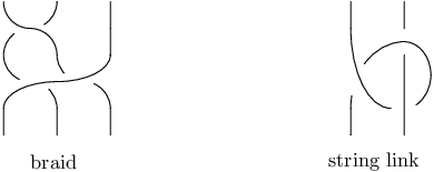
From a pure string link $L\subset D^{2}\times[0,1]$ with $g$ strings, we can construct a homology cylinder as follows. Recall the embedding $\iota:\Sigma_{0,g+1}\hookrightarrow\Sigma_{g,1}$ of a $g$ holed disk $\Sigma_{0,g+1}\subset D^{2}$ in Section 4.2 and Figure 3. Let $C$ be the complement of an open tubular neighborhood of $L$ in $D^{2}\times[0,1]$ . For any choice of a framing of $L$ , a homeomorphism $h:\partial C\xrightarrow{\cong}\partial(\iota(\Sigma_{0,g+1})\times[0,1])$ is fixed. (Note that a string link with a framing itself can be regarded as a homology cylinder over $\Sigma_{0,g+1}$ .) Then the manifold $M_{L}$ obtained from $\Sigma_{g,1}\times[0,1]$ by removing $\iota(\Sigma_{0,g+1})\times[0,1]$ and regluing $C$ by $h$ becomes a homology cylinder with the same marking as the trivial homology cylinder. This construction can be seen as a generalization of the embedding $P_{g}\hookrightarrow\mathcal{M}_{g,1}$ in Section 4.2 and it gives an injective monoid homomorphism from the monoid of pure string links to $\mathcal{C}_{g,1}$ . Moreover it induces an injective group homomorphism from the concordance group of pure string links with $g$ strings to $\mathcal{H}_{g,1}$ .

Habegger [46] gave another construction of homology cylinders from pure string links.

Example 5.7 ([40, 42]).

Let $K$ be a knot in $S^{3}$ with a Seifert surface $R$ of genus $g$ . By cutting open the knot exterior $E(K)$ along $R$ , we obtain a manifold $M_{R}$ . The boundary $\partial M_{R}$ is the union of two copies of $R$ glued along their boundary circles, which are just the knot $K$ . The pair $(M_{R},K)$ is called the complementary sutured manifold of $R$ . We can check that the following properties are equivalent to each other:

(a)

The Alexander polynomial $\Delta_{K}(t)$ is monic and its degree is equal to twice the genus of $g=g(K)$ of $K$ ;
(b)

The Seifert matrix $S$ of any minimal genus Seifert surface $R$ of $K$ is invertible over $\mathbb{Z}$ ;
(c)

The complementary sutured manifold $(M_{R},K)$ for any minimal genus Seifert surface $R$ is a homology product over $R$ .

We call a knot having the above properties a homologically fibered knot, where the name comes from the fact that fibered knots satisfy them. Thus if we fix an identification of $\Sigma_{g,1}$ with $R$ for a homologically fibered knot, we obtain a homology cylinder over $\Sigma_{g,1}$ . Note that aside from the name, the equivalence of the above conditions (a), (b), (c) was mentioned in Crowell-Trotter [30]. There exists a similar discussion for links.

We close this subsection by two observations on connections between homology cylinders and the theory of 3-manifolds.

First, the constructions of closed 3-manifolds mentioned in Section 4.6 have their analogue for homology cylinders. For example, the closure $C_{M}$ of a homology cylinder $(M,i_{+},i_{-})\in\mathcal{C}_{g,1}$ is defined as

C_{M}:=M/(i_{+}(x)=i_{-}(x))\quad x\in\Sigma_{g,1}.

By a topological consideration, we see that this construction is the same as gluing $\Sigma_{g,1}\times[0,1]$ to $M$ along their boundaries and also as the description of Habiro-Massuyeau [49, Definition 2.7]. The closure construction is compatible with the homology cobordism relation, denoted by H-cob, namely we have the following commutative diagram:

Therefore, roughly speaking, $\mathcal{H}_{g,1}$ might be regarded as a group structure on the set of homology cobordism classes of closed 3-manifolds. We have a similar discussion for clasper surgery equivalence.

Second, irreducibility of 3-manifolds often plays an important role in the theory of 3-manifolds (see Hempel’s book [56] for generalities). Correspondingly, we define:

Definition 5.8.

A homology cylinder $(M,i_{+},i_{-})\in\mathcal{C}_{g,1}$ is said to be irreducible if the underlying 3-manifold $M$ is irreducible. We denote by $\mathcal{C}_{g,1}^{\mathrm{irr}}$ the subset of $\mathcal{C}_{g,1}$ consisting of all irreducible homology cylinders.

By a standard argument using irreducibility, we can show that $\mathcal{C}_{g,1}^{\mathrm{irr}}$ is a submonoid of $\mathcal{C}_{g,1}$ . In particular, $\mathcal{C}_{0,0}^{\mathrm{irr}}\cong\mathcal{C}_{0,1}^{\mathrm{irr}}\cong\{1\}$ . Irreducible homology cylinders are all Haken manifolds since $|H_{1}(M)|=\infty$ for any $M\in\mathcal{C}_{g,n}$ unless $(g,n)=(0,0),(0,1)$ ,

For every $(M,i_{+},i_{-})\in\mathcal{C}_{g,1}$ , the underlying 3-manifold $M$ has a prime decomposition of the form

M\cong M_{0}\sharp X_{1}\sharp X_{2}\sharp\cdots\sharp X_{n},

where $M_{0}$ is the unique prime factor having $\partial M$ and $X_{1},X_{2},\ldots,X_{n}$ are homology 3-spheres. Note that $(M_{0},i_{+},i_{-})\in\mathcal{C}_{g,1}^{\mathrm{irr}}$ . Using Myers’ theorem [91, Theorem 3.2], we have the following description on the homology cobordism group of irreducible homology cylinders:

Proposition 5.9.

Every homology cylinder in $\mathcal{C}_{g,1}$ with $g\geq 1$ is homology cobordant to an irreducible one. That is,

\mathcal{C}_{g,1}^{\mathrm{irr}}/(\mbox{$\mathrm{H}$-$\mathrm{cob}$.})=\mathcal{H}_{g,1}.

5.2 Stallings’ theorem and the Johnson filtration

From now on, we limit our discussion to the case where $n=1$ as in the first part of this chapter. In this subsection, we briefly recall how to extend the (reduced versions of) Dehn-Nielsen embedding and Johnson homomorphisms to homology cylinders.

Convention.

We use the point $p\in\partial\Sigma_{g,1}$ as the common base point of $\Sigma_{g,1}$ , $i_{+}(\Sigma_{g,1})$ , $i_{-}(\Sigma_{g,1})$ , a homology cylinder $M$ , etc.

For a given $(M,i_{+},i_{-})\in\mathcal{C}_{g,1}$ , two homomorphisms $i_{+},i_{-}:\pi_{1}\Sigma_{g,1}\to\pi_{1}M$ are not generally isomorphisms. However, the following holds:

Theorem 5.10 (Stallings [110]).

Let $A$ and $B$ be groups and $f:A\rightarrow B$ be a $2$ -connected homomorphism. Then the induced map $f:N_{k}(A)\longrightarrow N_{k}(B)$ is an isomorphism for each $k\geq 2$ .

Here, a homomorphism $f:A\to B$ is said to be $2$ -connected if $f$ induces an isomorphism on the first homology, and an epimorphism on the second homology. In this chapter, the words ‘‘Stallings’ theorem’’ always means Theorem 5.10. Using the epimorphism (2.1), we can see that two homomorphisms $i_{+},i_{-}:\pi=\pi_{1}\Sigma_{g,1}\rightarrow\pi_{1}M$ are both $2$ -connected for any $(M,i_{+},i_{-})\in\mathcal{C}_{g,1}$ . Therefore, they induce isomorphisms on the nilpotent quotients of $\pi$ and $\pi_{1}M$ . For each $k\geq 2$ , we can define a map $\sigma_{k}:\mathcal{C}_{g,1}\rightarrow\mathrm{Aut}\,(N_{k}(\pi))$ by

\sigma_{k}(M,i_{+},i_{-}):=(i_{+})^{-1}\circ i_{-},

which gives a monoid homomorphism. It can be checked that $\sigma_{k}(M,i_{+},i_{-})$ depends only on the homology cobordism class of $(M,i_{+},i_{-})$ , so that we have a group homomorphism $\sigma_{k}:\mathcal{H}_{g,1}\rightarrow\mathrm{Aut}\,(N_{k}(\pi))$ . The restriction of $\sigma_{k}$ to the subgroup $\mathcal{M}_{g,1}\subset\mathcal{C}_{g,1}$ coincides with the homomorphism $\sigma_{k}$ mentioned in Section 4.5. The homomorphisms $\sigma_{k}$ $(k=2,3,\ldots)$ define filtrations

	$\displaystyle\mathcal{C}_{g,1}[1]$	$\displaystyle:=\mathcal{C}_{g,1}\supset\mathcal{C}_{g,1}[2]\supset\mathcal{C}_{g,1}[3]\supset\mathcal{C}_{g,1}[4]\supset\cdots$
	$\displaystyle\mathcal{H}_{g,1}[1]$	$\displaystyle:=\mathcal{H}_{g,1}\supset\mathcal{H}_{g,1}[2]\supset\mathcal{H}_{g,1}[3]\supset\mathcal{H}_{g,1}[4]\supset\cdots$

called the Johnson filtration of $\mathcal{C}_{g,1}$ and $\mathcal{H}_{g,1}$ by setting $\mathcal{C}_{g,1}[k]:=\mathop{\mathrm{Ker}}\nolimits\sigma_{k}$ and $\mathcal{H}_{g,1}[k]:=\mathop{\mathrm{Ker}}\nolimits\sigma_{k}$ .

By definition, the image of the homomorphism $\sigma_{k}$ is included in

\mathrm{Aut}_{0}(N_{k}(\pi)):=\left\{\varphi\in\mathrm{Aut}\,(N_{k}(\pi))\biggm|\begin{array}[]{c}\mbox{There exists a lift $\widetilde{\varphi}\in\operatorname{End}\pi$ of $\varphi$}\\ \mbox{satisfying $\widetilde{\varphi}(\zeta)\equiv\zeta\bmod\Gamma^{k+1}(\pi)$.}\end{array}\right\}.

On the other hand, Garoufalidis-Levine and Habegger independently showed the following:

Theorem 5.11 (Garoufalidis-Levine [35], Habegger [46]).

For $k\geq 2$ , the image of $\sigma_{k}$ coincides with $\mathrm{Aut}_{0}(N_{k}(\pi))$ .

As seen in Section 4.5, the $k$ -th Johnson homomorphism is obtained by restricting $\sigma_{k+2}$ to $\mathcal{C}_{g,1}[k+1]$ and $\mathcal{H}_{g,1}[k+1]$ . Garoufalidis-Levine [35, Proposition 2.5] showed that Andreadakis’ exact sequence in Section 4.5 (with $k$ shifted) restricts to the exact sequence

1\longrightarrow\mathfrak{h}_{g,1}(k)\longrightarrow\mathrm{Aut}_{0}(N_{k+2}(\pi))\longrightarrow\mathrm{Aut}_{0}(N_{k+1}(\pi))\longrightarrow 1.

Here $\mathfrak{h}_{g,1}(k)\subset\operatorname{Hom}(H,\Gamma^{k+1}(\pi)/\Gamma^{k+2}(\pi))$ is defined as the kernel of the composition

	$\displaystyle\operatorname{Hom}(H,\Gamma^{k+1}(\pi)/\Gamma^{k+2}(\pi))$	$\displaystyle\cong H^{\ast}\otimes(\Gamma^{k+1}(\pi)/\Gamma^{k+2}(\pi))$
		$\displaystyle\cong H\otimes(\Gamma^{k+1}(\pi)/\Gamma^{k+2}(\pi))$
		$\displaystyle=(\Gamma^{1}(\pi)/\Gamma^{2}(\pi))\otimes(\Gamma^{k+1}(\pi)/\Gamma^{k+2}(\pi))$
		$\displaystyle\to\Gamma^{k+2}(\pi)/\Gamma^{k+3}(\pi),$

where we used the Poincaré duality $H^{\ast}=H$ in the second row and the last map is obtained by taking commutators.

Corollary 5.12.

The $k$ -th Johnson homomorphisms $\tau_{k}:\mathcal{C}_{g,1}[k+1]\to\mathfrak{h}_{g,1}(k)$ and $\tau_{k}:\mathcal{H}_{g,1}[k+1]\to\mathfrak{h}_{g,1}(k)$ are surjective for any $k\geq 1$ .

Recall that in the case of the mapping class group, all the $\sigma_{k}:\mathcal{M}_{g,1}\to\mathrm{Aut}\,(N_{k}(\pi))$ for $k\geq 2$ are induced from a single homomorphism $\sigma:\mathcal{M}_{g,1}\to\mathrm{Aut}\,\pi$ . Then we pose the following question: Does there exist a homomorphism $\mathcal{H}_{g,1}\to\mathrm{Aut}\,\,G$ for some group $G$ which induces $\sigma_{k}:\mathcal{H}_{g,1}\to\mathrm{Aut}\,(N_{k}(\pi))$ for all $k\geq 2$ ? One of the answers is to use the map $\sigma^{\mathrm{nil}}:\mathcal{H}_{g,1}\to\mathrm{Aut}\,(\pi^{\mathrm{nil}})$ obtained by combining the homomorphisms $\sigma_{k}$ for all $k\geq 2$ , where $\pi^{\mathrm{nil}}:=\varprojlim_{k}N_{k}(\pi)$ is the nilpotent completion of $\pi$ . In fact, it was shown by Bousfield [15] that $N_{k}(G)\cong N_{k}(G^{\mathrm{nil}})$ holds for any finitely generated group $G$ and hence we have a natural homomorphism $\mathrm{Aut}\,(G^{\mathrm{nil}})\to\mathrm{Aut}\,(N_{k}(G))$ . However, $G^{\mathrm{nil}}$ is in general enormous and difficult to treat. In Section 6, we introduce the acyclic closure (or HE-closure) $G^{\mathrm{acy}}$ of a group $G$ as a reasonable extension and apply it to our situation.

6 Magnus representations for homology cylinders I

In this section, we extend the (universal) Magnus representation $r$ to $\mathcal{C}_{g,1}$ and $\mathcal{H}_{g,1}$ . The construction is based on Le Dimet’s argument [70] for the extension of the Gassner representation for string links. However what we present here is its generalized version: We construct our extended representations as crossed homomorphisms and use more general (not necessarily commutative) rings.

In the construction, there are two key ingredients: the acyclic closure of a group $G$ and the Cohn localization $\Lambda_{G}$ of $\mathbb{Z}[G]$ . The former is used to give a generalization of the Dehn-Nielsen theorem with no reduction and then we construct the (universal) Magnus representation $r$ for $\mathcal{C}_{g,1}$ and $\mathcal{H}_{g,1}$ with the aid of the latter.

6.1 Observation on fundamental groups of homology cylinders

The definition of the acyclic closure of a group is given purely in terms of group theory, whose relationship to topology seems to be unclear at first glance. Here we digress and give an observation to see the background.

For a homology cylinder $(M,i_{+},i_{-})\in\mathcal{C}_{g,1}$ , if we could have a natural assignment of an automorphism of $\pi$ , there would be no problem. However, it seems in general difficult (maybe impossible) to do so because $\pi_{1}M$ can be “bigger” than $\pi_{1}\Sigma_{g,1}$ :

The observation we now start is intended to give an “estimation” of how big $\pi_{1}M$ can be.

The usual handle decomposition theory and Morse theory say that $M$ , a homology cobordism over $\Sigma_{g,1}$ , is obtained from $\Sigma_{g,1}\times[0,1]$ by attaching a number of $1$ -handles $h_{1}^{1},h_{2}^{1},\ldots,h_{m}^{1}$ and the same number of $2$ -handles $h_{1}^{2},h_{2}^{2},\ldots,h_{m}^{2}$ to $\Sigma_{g,1}\times\{1\}$ . Then $\pi_{1}M$ can be written as

\pi_{1}M\cong\frac{\pi\ast\langle x_{1},x_{2},\ldots,x_{m}\rangle}{\langle r_{1},r_{2},\ldots,r_{m}\rangle},

where $x_{i}$ corresponds to attaching $h_{i}^{1}$ and $r_{j}$ to $h_{j}^{2}$ , and $\pi\ast\langle x_{1},x_{2},\ldots,x_{m}\rangle$ denotes the free product of $\pi$ and $\langle x_{1},x_{2},\ldots,x_{m}\rangle$ . Put $F_{m}=\langle x_{1},x_{2},\ldots,x_{m}\rangle$ . The condition $H_{\ast}(M,i_{-}(\Sigma_{g,1}))=0$ implies that the image of $\{r_{1},r_{2},\ldots,r_{m}\}$ under the map

\pi\ast F_{m}\xrightarrow{\mathrm{proj.}}F_{m}\longrightarrow H_{1}(F_{m})

forms a basis of $H_{1}(F_{m})\cong\mathbb{Z}^{m}$ . Repeating Tietze transformations, we can rewrite the above presentation into one of the form

\pi_{1}M\cong\frac{\pi\ast F_{m}}{\langle x_{1}v_{1}^{-1},x_{2}v_{2}^{-1},\ldots,x_{m}v_{m}^{-1}\rangle}

with $v_{j}\in\mathop{\mathrm{Ker}}\nolimits(\pi\ast F_{m}\xrightarrow{\mathrm{proj.}}F_{m}\longrightarrow H_{1}(F_{m}))$ for $j=1,2,\ldots,m$ .

On the other hand, given a group of the form

G=\frac{\pi\ast F_{m}}{\langle x_{1}w_{1}^{-1},x_{2}w_{2}^{-1},\ldots,x_{m}w_{m}^{-1}\rangle}

(6.5)

with $w_{j}\in\mathop{\mathrm{Ker}}\nolimits(\pi\ast F_{m}\xrightarrow{\mathrm{proj.}}F_{m}\to H_{1}(F_{m}))$ for $j=1,2,\ldots,m$ , we can construct a cobordism $W$ over $\Sigma_{g,1}\times[0,1]$ with $\pi_{1}W\cong G$ by attaching ( $4$ -dimensional) 1-handles $h_{1}^{1},h_{2}^{1},\ldots,h_{m}^{1}$ and $2$ -handles $h_{1}^{2},h_{2}^{2},\ldots,h_{m}^{2}$ to $(\Sigma_{g,1}\times[0,1])\times\{1\}\subset(\Sigma_{g,1}\times[0,1])\times[0,1]$ according to the words $x_{i}w_{i}^{-1}$ . We denote by $M$ the opposite side of $(\Sigma_{g,1}\times[0,1])\times\{0\}$ in $\partial W$ , namely $\partial W=(\Sigma_{g,1}\times[0,1])\cup(-M)$ . By construction, the manifold $M$ with the same markings as $(\Sigma_{g,1}\times[0,1],\mathop{\mathrm{id}}\nolimits\times 1,\mathop{\mathrm{id}}\nolimits\times 0)$ defines a homology cylinder in $\mathcal{C}_{g,1}$ and $W$ is a homology cobordism between $M$ and $\Sigma_{g,1}\times[0,1]$ . By the duality of handle decompositions, the cobordism $W$ is also obtained from $M\times[0,1]$ by attaching $2$ -handles and $3$ -handles. Therefore we have a surjective homomorphism $\pi_{1}M\twoheadrightarrow\pi_{1}W\cong G$ . That is, roughly speaking, $\pi_{1}M$ is “bigger” than $G$ . (In higher-dimensional cases discussed in Section 8.4, we have an isomorphism $\pi_{1}M\cong G$ .) Consequently, we have:

Proposition 6.1.

The fundamental group $\pi_{1}M$ of $(M,i_{+},i_{-})\in\mathcal{C}_{g,1}$ can be written in the form $(\ref{eq:pi1})$ for some $m$ with $w_{j}$ ’s in $\mathop{\mathrm{Ker}}\nolimits(\pi\ast F_{m}\xrightarrow{\mathrm{proj.}}F_{m}\to H_{1}(F_{m}))$ . Conversely, for any group $G$ having such a form, there exists a homology cylinder $(M,i_{+},i_{-})\in\mathcal{C}_{g,1}$ such that $\pi_{1}M$ surjects onto $G$ .

6.2 The acyclic closure of a group

The concept of the acyclic closure (or HE-closure in [72]) of a group was defined as a variation of the algebraic closure of a group by Levine [71, 72]. Topologically, the algebraic (acyclic) closure of a group $G$ can be obtained as the fundamental group of (a variation of) the Vogel localization of any CW-complex $X$ with $\pi_{1}X\cong G$ (see Le Dimet’s book [69]). We summarize here the definition and fundamental properties. We also refer to Hillman’s book [57] and Cha’s paper [20]. The proofs of the propositions in this subsection are almost the same as those for the algebraic closures in [71].

Definition 6.2.

Let $G$ be a group, and let $F_{m}=\langle x_{1},x_{2},\ldots,x_{m}\rangle$ be a free group of rank $m$ .
(i) $w=w(x_{1},x_{2},\ldots,x_{m})\in G\ast F_{m}$ , a word in $x_{1},x_{2},\ldots,x_{m}$ and elements of $G$ , is said to be acyclic if

w\in\mathop{\mathrm{Ker}}\nolimits\left(G\ast F_{m}\xrightarrow{\mathrm{proj}}F_{m}\longrightarrow H_{1}(F_{m})\right).

(ii) Consider the following “equation” with variables $x_{1},x_{2},\ldots,x_{m}$ :

\left\{\begin{array}[]{ccl}x_{1}&=&w_{1}(x_{1},x_{2},\ldots,x_{m})\\ x_{2}&=&w_{2}(x_{1},x_{2},\ldots,x_{m})\\ &\vdots&\\ x_{m}&=&w_{m}(x_{1},x_{2},\ldots,x_{m})\end{array}\right..

When all words $w_{1},w_{2},\ldots,w_{m}\in G\ast F_{m}$ are acyclic, we call such an equation an acyclic system over $G$ .
(iii) A group $G$ is said to be acyclically closed (AC, for short) if every acyclic system over $G$ with $m$ variables has a unique “solution” in $G$ for any $m\geq 0$ , where a “solution” means a homomorphism $\varphi$ that makes the following diagram commutative:

Example 6.3.

Let $G$ be an abelian group. For $g_{1},g_{2},g_{3}\in G$ , consider the equation

\left\{\begin{array}[]{l}x_{1}=g_{1}x_{1}g_{2}x_{2}x_{1}^{-1}x_{2}^{-1}\\ x_{2}=x_{1}g_{3}x_{1}^{-1}\end{array}\right.,

which is an acyclic system. Then we have a unique solution $x_{1}=g_{1}g_{2},\,x_{2}=g_{3}$ .

As we can expect from this example, all abelian groups are AC. Moreover, all nilpotent groups and the nilpotent completion of a group are AC, which can be deduced from the following fundamental properties of AC-groups:

Proposition 6.4 ([71, Proposition 1]).

${\rm(a)}$ Let $\{G_{\alpha}\}_{\alpha}$ be a family of AC-subgroups of an AC-group $G$ . Then $\bigcap_{\alpha}G_{\alpha}$ is also an AC-subgroup of $G$ .
${\rm(b)}$ Let $\{G_{\alpha}\}_{\alpha}$ be a family of AC-groups. Then $\prod_{\alpha}G_{\alpha}$ is also an AC-group.
${\rm(c)}$ When $G$ is a central extension of $H$ , then $G$ is an AC-group if and only if $H$ is an AC-group.
${\rm(d)}$ For any direct system $($ resp. inverse system $)$ of AC-groups, the direct limit $($ resp. inverse limit $)$ is also an AC-group.

Let us define the acyclic closure of a group.

Proposition 6.5 ([71, Proposition 3]).

For any group $G$ , there exists a pair of a group $G^{\mathrm{acy}}$ and a homomorphism $\iota_{G}:G\rightarrow G^{\mathrm{acy}}$ satisfying the following properties:

1.

$G^{\mathrm{acy}}$ is an AC-group.
2.

Let $f:G\rightarrow A$ be a homomorphism and suppose that $A$ is an AC-group. Then there exists a unique homomorphism $f^{\mathrm{acy}}:G^{\mathrm{acy}}\rightarrow A$ which satisfies $f^{\mathrm{acy}}\circ\iota_{G}=f$ .

Moreover such a pair is unique up to isomorphism.

Definition 6.6.

We call $\iota_{G}$ (or $G^{\mathrm{acy}}$ ) obtained above the acyclic closure of $G$ .

Taking the acyclic closure of a group is functorial, namely, for each group homomorphism $f:G_{1}\to G_{2}$ , we have the induced homomorphism $f^{\mathrm{acy}}:G_{1}^{\mathrm{acy}}\to G_{2}^{\mathrm{acy}}$ by applying the universal property of $G_{1}^{\mathrm{acy}}$ to the homomorphism $\iota_{G_{2}}\circ f$ , and the composition of homomorphisms induces that of the corresponding homomorphisms on acyclic closures.

The most important properties of the acyclic closure are the following:

Proposition 6.7 ([71, Proposition 4]).

For every group $G$ , the acyclic closure $\iota_{G}:G\rightarrow G^{\mathrm{acy}}$ is $2$ -connected.

Proposition 6.8 ([71, Proposition 5]).

Let $G$ be a finitely generated group and $H$ a finitely presentable group. For each $2$ -connected homomorphism $f:G\rightarrow H$ , the induced homomorphism $f^{\mathrm{acy}}:G^{\mathrm{acy}}\to H^{\mathrm{acy}}$ on acyclic closures is an isomorphism.

From Proposition 6.7 and Stallings’ theorem, the nilpotent quotients of a group and those of its acyclic closure are isomorphic. Note that the homomorphism $\iota_{G}$ is not necessarily injective: consider a perfect group $G$ and the 2-connected homomorphism $G\to\{1\}$ . As for a free group $F_{m}$ , its residual nilpotency shows that $\iota_{F_{m}}$ is injective.

Proposition 6.9 ([71, Proposition 6]).

For any finitely presentable group $G$ , there exists a sequence of finitely presentable groups and homomorphisms

G=P_{0}\rightarrow P_{1}\rightarrow P_{2}\rightarrow\cdots\rightarrow P_{k}\rightarrow P_{k+1}\rightarrow\cdots

satisfying the following properties:

1.

$G^{\mathrm{acy}}=\displaystyle\varinjlim_{k}P_{k}$ , and $\iota_{G}:G\rightarrow G^{\mathrm{acy}}$ coincides with the limit map of the above sequence.
2.

$G\rightarrow P_{k}$ is a $2$ -connected homomorphism for any $k\geq 1$ .

From this proposition, we see, in particular, that the acyclic closure of a finitely presentable group is a countable set.

6.3 Dehn-Nielsen type theorem

Now we return to our discussion on homology cylinders. For each homology cylinder $(M,i_{+},i_{-})\in\mathcal{C}_{g,1}$ , we have a commutative diagram

\begin{CD}\pi @>{i_{-}}>{}>\pi_{1}M@<{i_{+}}<{}<\pi\\ @V{\iota_{\pi}}V{}V@V{\iota_{\pi_{1}M}}V{}V@V{}V{\iota_{\pi}}V\\ \pi^{\mathrm{acy}}@>{i_{-}^{\mathrm{acy}}}>{\cong}>(\pi_{1}M)^{\mathrm{acy}}@<{i_{+}^{\mathrm{acy}}}<{\cong}<\pi^{\mathrm{acy}}\end{CD}

by Proposition 6.8. From this, we obtain a monoid homomorphism defined by

\sigma^{\mathrm{acy}}:\mathcal{C}_{g,1}\longrightarrow\mathrm{Aut}\,(\pi^{\mathrm{acy}})\qquad\left(\,(M,i_{+},i_{-})\mapsto(i_{+}^{\mathrm{acy}})^{-1}\circ i_{-}^{\mathrm{acy}}\,\right)

and it induces a group homomorphism $\sigma^{\mathrm{acy}}:\mathcal{H}_{g,1}\rightarrow\mathrm{Aut}\,(\pi^{\mathrm{acy}})$ .

Here we describe a generalization of the Dehn-Nielsen theorem. Recall that $\zeta\in\pi\subset\pi^{\mathrm{acy}}$ is a word corresponding to the boundary loop of $\Sigma_{g,1}$ .

Theorem 6.10 ([103, Theorem 6.1]).

The image of $\sigma^{\mathrm{acy}}:\mathcal{H}_{g,1}\to\mathrm{Aut}\,(\pi^{\mathrm{acy}})$ is

\mathrm{Aut}_{0}(\pi^{\mathrm{acy}}):=\{\varphi\in\mathrm{Aut}\,(\pi^{\mathrm{acy}})\mid\varphi(\zeta)=\zeta\in\pi^{\mathrm{acy}}\}.

In the proof, we immediately see that the image of $\sigma^{\mathrm{acy}}$ is included in $\mathrm{Aut}_{0}(\pi^{\mathrm{acy}})$ since $i_{+}(\zeta)=i_{-}(\zeta)\in\pi_{1}M$ for every $(M,i_{+},i_{-})\in\mathcal{C}_{g,1}$ . Conversely, given an element $\varphi\in\mathrm{Aut}_{0}(\pi^{\mathrm{acy}})$ , we need to construct a homology cylinder $M=(M,i_{+},i_{-})$ satisfying $\sigma^{\mathrm{acy}}(M)=\varphi$ . The construction is based on that of Theorem 5.11 [35, Theorem 3] due to Garoufalidis-Levine. In our context, however, we must pay extra attention because there is a difference between our situation and theirs: Although the composition $\pi\to\pi^{\mathrm{acy}}\to N_{k}(\pi^{\mathrm{acy}})\cong N_{k}(\pi)$ is surjective, $\iota_{\pi}:\pi\to\pi^{\mathrm{acy}}$ is not.

Note that $\mathcal{H}_{g,1}[[\infty]]:=\mathop{\mathrm{Ker}}\nolimits(\sigma^{\mathrm{acy}})$ is non-trivial in contrast with the case of the mapping class group. Indeed the homology cobordism group $\Theta_{\mathbb{Z}}^{3}$ of homology 3-spheres is included in it. See also Section 8.2 for more about $\mathcal{H}_{g,1}[[\infty]]$ . As for the mysterious group $\mathcal{H}_{g,1}[[\infty]]$ , we have the following problem:

Problem 6.11.

Determine whether $\mathcal{H}_{g,1}[[\infty]]$ coincides with the group

	$\displaystyle\mathcal{H}_{g,1}[\infty]:=$	$\displaystyle\bigcap_{k\geq 2}\mathop{\mathrm{Ker}}\nolimits(\sigma_{k}:\mathcal{H}_{g,1}\to\mathrm{Aut}\,(N_{k}(\pi)))$
	$\displaystyle=$	$\displaystyle\mathop{\mathrm{Ker}}\nolimits(\sigma^{\mathrm{nil}}:\mathcal{H}_{g,1}\to\mathrm{Aut}\,(\pi^{\mathrm{nil}})),$

in which $\mathcal{H}_{g,1}[[\infty]]$ is included. This is closely related to the question whether the natural map $\pi^{\mathrm{acy}}\to\pi^{\mathrm{nil}}$ is injective or not.

6.4 Extension of the Magnus representation

As in the original case, the (universal) Magnus representation for homology cylinders is obtained from that for $\mathrm{Aut}\,(F^{\mathrm{acy}}_{n})$ through the Dehn-Nielsen type theorem. The resulting representation is also a crossed homomorphism.

For the construction, we need another tool called (a special case of) the Cohn localization or the universal localization. We refer to [29, Section 7] for details.

Proposition 6.12 (Cohn [29]).

Let $G$ be a group with the trivializer $\mathfrak{t}:\mathbb{Z}[G]\to\mathbb{Z}$ . Then there exists a pair of a ring $\Lambda_{G}$ and a ring homomorphism $l_{G}:\mathbb{Z}[G]\to\Lambda_{G}$ satisfying the following properties:

1.

For every matrix $m$ with coefficients in $\mathbb{Z}[G]$ , if ${}^{\mathfrak{t}}m$ is invertible then ${}^{l_{G}}m$ is also invertible.
2.

The pair $(\Lambda_{G},l_{G})$ is universal among all pairs having the property $(1)$ .

Furthermore the pair $(\Lambda_{G},l_{G})$ is unique up to isomorphism.

Note that any automorphism of a group $G$ induces an automorphism of $\mathbb{Z}[G]$ and moreover of $\Lambda_{G}$ by the universal property of $\Lambda_{G}$ .

Example 6.13.

When $G=H_{1}(F_{n})$ , we have

\Lambda_{H_{1}(F_{n})}\cong\left\{\,\displaystyle\frac{f}{g}\,\biggm|f,g\in\mathbb{Z}[H_{1}(F_{n})],\ \mathfrak{t}(g)=\pm 1\right\}.

We write $\gamma_{i}$ again for the image of $\gamma_{i}$ by $\iota_{F_{n}}:F_{n}=\langle\gamma_{1},\gamma_{2},\ldots,\gamma_{n}\rangle\hookrightarrow F^{\mathrm{acy}}_{n}$ . Now we can check the following facts on $\Lambda_{F^{\mathrm{acy}}_{n}}$ :

Lemma 6.14.

$(1)$ The composition $\mathbb{Z}[F_{n}]\xrightarrow{\iota_{F_{n}}}\mathbb{Z}[F^{\mathrm{acy}}_{n}]\xrightarrow{l_{F^{\mathrm{acy}}_{n}}}\Lambda_{F^{\mathrm{acy}}_{n}}$ is injective.

$(2)$ Let $G$ be a finitely presentable group and let $f:F_{n}\to G$ be a $2$ -connected homomorphism. Then $H_{i}(G,f(F_{n});\Lambda_{G})=0$ holds for $i=0,1,2$ . Moreover, we may take $F^{\mathrm{acy}}_{n}$ as $G$ .

Sketch of Proof.

Consider the composition of the ring homomorphism $\mathbb{Z}[F^{\mathrm{acy}}_{n}]\to\mathbb{Z}[F_{n}^{\mathrm{nil}}]$ with the Magnus expansion, which can be extended to $\mathbb{Z}[F_{n}^{\mathrm{nil}}]$ . It is known that the Magnus expansion is injective on $\mathbb{Z}[F_{n}]$ . We can check that this composition satisfies Property $(1)$ of Proposition 6.12, so that the Magnus expansion can be extended to $\Lambda_{F^{\mathrm{acy}}_{n}}$ . Hence $(1)$ follows.

For the proof of the first assertion of $(2)$ , see [103, Lemma 5.11]. We may put $G=F^{\mathrm{acy}}_{n}$ by Proposition 6.9 and commutativity of homology and direct limits. ∎

Lemma 6.14 $(2)$ leads us to show the following, which can be regarded as a generalization of the isomorphism (2.2). The proof is almost the same as that of [70, Proposition 1.1].

Proposition 6.15.

The homomorphism

\chi:\Lambda_{F^{\mathrm{acy}}_{n}}^{n}\longrightarrow I(F^{\mathrm{acy}}_{n})\otimes_{\mathbb{Z}[F^{\mathrm{acy}}_{n}]}\Lambda_{F^{\mathrm{acy}}_{n}}

sending $(a_{1},\ldots,a_{n})^{T}\in\Lambda_{F^{\mathrm{acy}}_{n}}^{n}$ to $\displaystyle\sum_{i=1}^{n}(\gamma_{i}^{-1}-1)\otimes a_{i}$ is an isomorphism of right $\Lambda_{F^{\mathrm{acy}}_{n}}$ -modules, where $I(F^{\mathrm{acy}}_{n}):=\mathop{\mathrm{Ker}}\nolimits(\mathfrak{t}:\mathbb{Z}[F^{\mathrm{acy}}_{n}]\to\mathbb{Z})$ .

Definition 6.16.

For $1\leq i\leq n$ , we define the extended Fox derivative

\frac{\partial}{\partial\gamma_{i}}:F^{\mathrm{acy}}_{n}\longrightarrow\Lambda_{F^{\mathrm{acy}}_{n}}

by the formula

\begin{array}[]{rccc}\left(\displaystyle\frac{\partial}{\partial\gamma_{1}},\frac{\partial}{\partial\gamma_{2}},\ldots,\frac{\partial}{\partial\gamma_{n}}\right)^{T}:&F^{\mathrm{acy}}_{n}&\longrightarrow&\Lambda_{F^{\mathrm{acy}}_{n}}^{n}\\ &\mbox{\rotatebox[origin={c}]{90.0}{$\in$}}&&\mbox{\rotatebox[origin={c}]{90.0}{$\in$}}\\ &v&\longmapsto&\overline{\chi^{-1}((v^{-1}-1)\otimes 1)}.\end{array}

The extended Fox derivatives coincide with the original ones if we restrict them to $F_{n}$ (cf. Example 2.10). They share many properties as mentioned in [70, Proposition 1.3]. In particular, we have the equality

(v^{-1}-1)\otimes 1=\sum_{i=1}^{n}(\gamma_{i}^{-1}-1)\otimes\overline{\left(\frac{\partial v}{\partial\gamma_{i}}\right)}\ \ \in I(F^{\mathrm{acy}}_{n})\otimes_{\mathbb{Z}[F^{\mathrm{acy}}_{n}]}\Lambda_{F^{\mathrm{acy}}_{n}}

for any $v\in F^{\mathrm{acy}}_{n}$ .

Definition 6.17.

The $($ universal $)$ Magnus representation for $\mathrm{Aut}\,(F^{\mathrm{acy}}_{n})$ is the map

r:\mathrm{Aut}\,(F^{\mathrm{acy}}_{n})\to M(n,\Lambda_{F^{\mathrm{acy}}_{n}})

assigning to $\varphi\in\mathrm{Aut}\,(F^{\mathrm{acy}}_{n})$ the matrix

r(\varphi):=\left(\overline{\left(\frac{\partial\varphi(\gamma_{j})}{\partial\gamma_{i}}\right)}\right)_{i,j}.

We can easily check that the Magnus representation $r$ is a crossed homomorphism and the image of $r$ is included in the set $\mathrm{GL}(n,\Lambda_{F^{\mathrm{acy}}_{n}})$ of invertible matrices. By Lemma 6.14 $(1)$ , we see that the Magnus representation defined here gives a generalization of the original.

Example 6.18.

Consider the monoid $\operatorname{End}_{2}(F_{n})$ of all $2$ -connected endomorphisms of $F_{n}$ . We have a natural homomorphism $\operatorname{End}_{2}(F_{n})\to\mathrm{Aut}\,(F^{\mathrm{acy}}_{n})$ by Proposition 6.8. For any $f\in\operatorname{End}_{2}(F_{n})$ , the Magnus matrix $r(f)$ can be obtained by using the original Fox derivatives. In particular, $r$ is injective on $\operatorname{End}_{2}(F_{n})$ . Therefore, we see that $\operatorname{End}_{2}(F_{n})$ is a submonoid of $\mathrm{Aut}\,(F^{\mathrm{acy}}_{n})$ . Every automorphism of $\mathrm{Aut}\,(N_{k}(F_{n}))$ can be lifted to a $2$ -connected endomorphism of $F_{n}$ . Hence the homomorphisms $\mathrm{Aut}\,(F^{\mathrm{acy}}_{n})\to\mathrm{Aut}\,(N_{k}(F^{\mathrm{acy}}_{n}))\cong\mathrm{Aut}\,(N_{k}(F_{n}))$ are surjective for all $k\geq 2$ .

Finally, by using the Dehn-Nielsen type theorem for $n=2g$ , we obtain the (universal) Magnus representation

r:\mathcal{C}_{g,1}\longrightarrow\mathrm{GL}(2g,\Lambda_{\pi^{\mathrm{acy}}})

for homology cylinders, which induces $r:\mathcal{H}_{g,1}\to\mathrm{GL}(2g,\Lambda_{\pi^{\mathrm{acy}}})$ .

7 Magnus representations for homology cylinders II

In this section, we discuss another method for extending Magnus representations by using twisted homology of homology cylinders. This time, we follow the Kirk-Livingston-Wang’s construction [66]. In connection with it, we also mention another invariant of homology cylinders arising from torsion.

For our purpose, we first recall the setting of higher-order Alexander invariants originating in Cochran-Orr-Teichner [27], Cochran [24] and Harvey [51, 52], where PTFA groups play an important role. A group $\Gamma$ is said to be poly-torsion-free abelian $($ PTFA $)$ if it has a sequence

\Gamma=\Gamma_{1}\triangleright\Gamma_{2}\triangleright\cdots\triangleright\Gamma_{n}=\{1\}

whose successive quotients $\Gamma_{i}/\Gamma_{i+1}$ $(i\geq 1)$ are all torsion-free abelian. An advantage of using PTFA groups is that the group ring $\mathbb{Z}[\Gamma]$ of $\Gamma$ is known to be an Ore domain so that it can be embedded into the field (skew field in general)

\mathcal{K}_{\Gamma}:=\mathbb{Z}[\Gamma](\mathbb{Z}[\Gamma]-\{0\})^{-1}

called the right field of fractions. We refer to the books of Cohn [29] and Passman [99] for generalities of localizations of non-commutative rings. A typical example of a PTFA group is $\mathbb{Z}^{n}$ , where $\mathcal{K}_{\mathbb{Z}^{n}}$ is isomorphic to the field of rational functions with $n$ variables. More generally, free nilpotent quotients $N_{k}(F_{n})$ and $N_{k}(\pi)$ are known to be PTFA.

Let $M=(M,i_{+},i_{-})\in\mathcal{C}_{g,1}$ . We fix a homomorphism $\rho:\pi_{1}M\to\Gamma$ into a PTFA group $\Gamma$ . The following lemma is crucial in our construction of Magnus matrices (cf. Lemma 6.14). For the direct proof, see [66, Proposition 2.1]. See also Cochran-Orr-Teichner [27, Section 2] for a more general treatment.

Lemma 7.1.

For $\pm\in\{+,-\}$ , we have $H_{\ast}(M,i_{\pm}(\Sigma_{g,1});\mathcal{K}_{\Gamma})=0$ . Equivalently,

i_{\pm}:H_{\ast}(\Sigma_{g,1},\{p\};i_{\pm}^{\ast}\mathcal{K}_{\Gamma})\longrightarrow H_{\ast}(M,\{p\};\mathcal{K}_{\Gamma})

is an isomorphism of right $\mathcal{K}_{\Gamma}$ -vector spaces.

Remark 7.2.

The same conclusion as in the above lemma holds for the homology with coefficients in any $\mathbb{Z}[\pi_{1}M]$ -algebra $\mathcal{R}$ satisfying: Every matrix with entries in $\mathbb{Z}[\pi_{1}M]$ sent to an invertible one by the trivializer $\mathfrak{t}:\mathbb{Z}[\pi_{1}M]\to\mathbb{Z}$ is also invertible in $\mathcal{R}$ (cf. Proposition 6.12). By a theorem of Strebel [111], we see that $\mathcal{K}_{\Gamma}$ satisfies this property for any homomorphism $\pi_{1}M\to\Gamma$ into a PTFA group $\Gamma$ .

Since $S:=\displaystyle\bigcup_{i=1}^{2g}\gamma_{i}\subset\Sigma_{g,1}$ (see Figure 1) is a deformation retract of $\Sigma_{g,1}$ relative to $p$ , we have $\pi\cong\pi_{1}S$ and

H_{1}(\Sigma_{g,1},\{p\};i_{\pm}^{\ast}\mathcal{K}_{\Gamma})\cong H_{1}(S,\{p\};i_{\pm}^{\ast}\mathcal{K}_{\Gamma})=C_{1}(\widetilde{S})\otimes_{\mathbb{Z}[\pi]}i_{\pm}^{\ast}\mathcal{K}_{\Gamma}\cong\mathcal{K}_{\Gamma}^{2g}

with basis $\{\widetilde{\gamma_{1}}\otimes 1,\ldots,\widetilde{\gamma_{2g}}\otimes 1\}\subset C_{1}(\widetilde{S})\otimes_{\mathbb{Z}[\pi]}i_{\pm}^{\ast}\mathcal{K}_{\Gamma}$ as a right $\mathcal{K}_{\Gamma}$ -vector space (see Section 4.2).

Definition 7.3.

For $M=(M,i_{+},i_{-})\in\mathcal{C}_{g,1}$ and a homomorphism $\pi_{1}M\to\Gamma$ into a PTFA group $\Gamma$ , the Magnus matrix $r_{\rho}(M)\in\mathrm{GL}(2g,\mathcal{K}_{\Gamma})$ associated with $\rho$ is defined as the representation matrix of the right $\mathcal{K}_{\Gamma}$ -isomorphism

	$\displaystyle\mathcal{K}_{\Gamma}^{2g}\cong H_{1}(\Sigma_{g,1},\{p\};i_{-}^{\ast}\mathcal{K}_{\Gamma})$	$\displaystyle\xrightarrow[\cong]{i_{-}}H_{1}(M,\{p\};\mathcal{K}_{\Gamma})$
		$\displaystyle\xrightarrow[\cong]{i_{+}^{-1}}H_{1}(\Sigma_{g,1},\{p\};i_{+}^{\ast}\mathcal{K}_{\Gamma})\cong\mathcal{K}_{\Gamma}^{2g},$

where the first and the last isomorphisms use the basis mentioned above.

A method for computing $r_{\rho}(M)$ is given in [40, Section 4], which is based on one of Kirk-Livingston-Wang [66]. An admissible presentation of $\pi_{1}M$ is defined to be one of the form

\displaystyle\langle i_{-}(\gamma_{1}),\ldots,i_{-}(\gamma_{2g}),z_{1},\ldots,z_{l},i_{+}(\gamma_{1}),\ldots,i_{+}(\gamma_{2g})\mid r_{1},\ldots,r_{2g+l}\rangle

(7.6)

for some integer $l\geq 0$ . That is, it is a finite presentation with deficiency $2g$ whose generating set contains $i_{-}(\gamma_{1}),\ldots,i_{-}(\gamma_{2g}),i_{+}(\gamma_{1}),\ldots,i_{+}(\gamma_{2g})$ and is ordered as above. Such a presentation always exists. For any admissible presentation, we define $2g\times(2g+l)$ , $l\times(2g+l)$ and $2g\times(2g+l)$ matrices $A,B,C$ by

A=\overline{\left(\frac{\partial r_{j}}{\partial i_{-}(\gamma_{i})}\right)}_{\begin{subarray}{c}{}1\leq i\leq 2g\\ 1\leq j\leq 2g+l\end{subarray}},\ B=\overline{\left(\frac{\partial r_{j}}{\partial z_{i}}\right)}_{\begin{subarray}{c}{}1\leq i\leq l\\ 1\leq j\leq 2g+l\end{subarray}},\ C=\overline{\left(\frac{\partial r_{j}}{\partial i_{+}(\gamma_{i})}\right)}_{\begin{subarray}{c}{}1\leq i\leq 2g\\ 1\leq j\leq 2g+l\end{subarray}}

over $\mathbb{Z}[\Gamma]\subset\mathcal{K}_{\Gamma}$ .

Proposition 7.4 ([40, Propositions 4.5, 4.6]).

The square matrix $\begin{pmatrix}A\\ B\end{pmatrix}$ is invertible over $\mathcal{K}_{\Gamma}$ and we have

r_{\rho}(M)=-C\begin{pmatrix}A\\ B\end{pmatrix}^{-1}\!\begin{pmatrix}I_{2g}\\ 0_{(l,2g)}\end{pmatrix}\in\mathrm{GL}(2g,\mathcal{K}_{\Gamma}).

(7.7)

Remark 7.5.

We shall meet the same formula (7.7) when we compute the Magnus matrix following the definition in the previous section. From this, we can conclude that the definitions in this and the previous sections are the same.

Formula (7.7) gives the following properties of Magnus matrices:

Proposition 7.6.

Let $\Gamma$ be a PTFA group.

(1)

For $\varphi\in\mathcal{M}_{g,1}\hookrightarrow\mathrm{Aut}\,\pi$ and a homomorphism $\rho:\pi_{1}(\Sigma_{g,1}\times[0,1])=\pi\to\Gamma$ , we have

r_{\rho}((\Sigma_{g,1}\times[0,1],\mathop{\mathrm{id}}\nolimits\times 1,\varphi\times 0))=\sideset{{}^{\rho}\!}{{}_{i,j}}{\mathop{\left({\overline{\left(\displaystyle\frac{\partial\varphi(\gamma_{j})}{\partial\gamma_{i}}\right)}}\right)}\nolimits}.

$(2)$

$($ Functoriality $)$ For $M,N\in\mathcal{C}_{g,1}$ and a homomorphism $\rho:\pi_{1}(M\cdot N)\to\Gamma$ , we have

$r_{\rho}(M\cdot N)=r_{\rho\circ i}(M)\cdot r_{\rho\circ j}(N),$

where $i:\pi_{1}M\to\pi_{1}(M\cdot N)$ and $j:\pi_{1}N\to\pi_{1}(M\cdot N)$ are the induced maps from the inclusions $M\hookrightarrow M\cdot N$ and $N\hookrightarrow M\cdot N$ .
$(3)$

$($ Homology cobordism invariance $)$ Suppose $M,N\in\mathcal{C}_{g,1}$ are homology cobordant by a homology cobordism $W$ . For any homomorphism $\rho:\pi_{1}W\to\Gamma$ , we have

$r_{\rho\circ i}(M)=r_{\rho\circ j}(N),$

where $i:\pi_{1}M\to\pi_{1}W$ and $j:\pi_{1}N\to\pi_{1}W$ are the induced maps from the inclusions $M\hookrightarrow W$ and $N\hookrightarrow W$ .

Hence Magnus matrices are invariants of pairs of a homology cylinder and a homomorphism $\rho$ . To obtain a map from a submonoid of $\mathcal{C}_{g,1}$ solely, we need a natural choice of $\rho$ for all homology cylinders involved that have some compatibility with respect to the product operation in $\mathcal{C}_{g,1}$ . For that purpose, we here use the nilpotent quotient $N_{k}(\pi)$ with fixed $k\geq 2$ . Using Stallings’ theorem, we can consider the composition

\mathfrak{q}_{k}:\pi_{1}M\longrightarrow N_{k}(\pi_{1}M)\xrightarrow[\cong]{i_{+}^{-1}}N_{k}(\pi)

for every $(M,i_{+},i_{-})\in\mathcal{C}_{g,1}$ . Then we have a map

r_{\mathfrak{q}_{k}}:\mathcal{C}_{g,1}\longrightarrow\mathrm{GL}(2g,\mathcal{K}_{N_{k}(\pi)})

and Proposition 7.6 can be rewritten as follows:

Proposition 7.7 ([105]).

Let $k\geq 2$ be an integer.

$(1)$

The map $r_{\mathfrak{q}_{k}}$ extends the corresponding Magnus representation for $\mathcal{M}_{g,1}$ .
$(2)$

The map $r_{\mathfrak{q}_{k}}$ is a crossed homomorphism, namely, the equality

$r_{\mathfrak{q}_{k}}(M_{1}\cdot M_{2})=r_{\mathfrak{q}_{k}}(M_{1})\cdot{}^{\sigma_{k}(M_{1})}(r_{\mathfrak{q}_{k}}(M_{2}))$

holds for any $M_{1},M_{2}\in\mathcal{C}_{g,1}$ by using $\sigma_{k}:\mathcal{C}_{g,1}\to\mathrm{Aut}\,(N_{k}(\pi))$ .
$(3)$

$r_{\mathfrak{q}_{k}}$ induces a crossed homomorphism $r_{\mathfrak{q}_{k}}:\mathcal{H}_{g,1}\to\mathrm{GL}(2g,\mathcal{K}_{N_{k}(\pi)})$ .

As in the case of $\mathcal{M}_{g,1}$ , the restrictions of $r_{\mathfrak{q}_{k}}$ to $\mathcal{C}_{g,1}[k]$ and $\mathcal{H}_{g,1}[k]$ give genuine homomorphisms.

We can naturally generalize the arguments in Sections 4.2 and 4.3. For example, the (twisted) symplecticity

\overline{r_{\mathfrak{q}_{k}}(M)^{T}}\ {}^{\mathfrak{q}_{k}}\!\widetilde{J}\ r_{\mathfrak{q}_{k}}(M)={}^{\sigma_{k}(M)}({}^{\mathfrak{q}_{k}}\!\widetilde{J})\in\mathrm{GL}(2g,\mathcal{K}_{N_{k}(\pi)})

(7.8)

holds. Note that the proof in [104] is also applicable to the universal Magnus representation $r$ .

Remark 7.8.

The author does not know whether we can define (crossed) homomorphisms from $\mathcal{C}_{g,1}$ and $\mathcal{H}_{g,1}$ by using derived quotients of $\pi_{1}M$ . This is because there are no results for derived quotients of groups corresponding completely to Stallings’ theorem except that Cochran-Harvey [25] gave a partial result, which was used to define homology cobordism invariants of 3-manifolds arising from $L^{2}$ -signature invariants (see Harvey [53] for example).

Example 7.9 ([105, Example 4.4]).

Let $L$ be the pure string link of Figure 5 with $2$ strings.

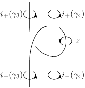
By Levine’s construction in Example 5.6, $L$ yields a homology cylinder $(M_{L},i_{+},i_{-})\in\mathcal{C}_{g,1}$ with $\pi_{1}M_{L}$ having an admissible presentation:

{\small\left\langle\begin{array}[]{c|c}\begin{array}[]{c}i_{-}(\gamma_{1}),\ldots,i_{-}(\gamma_{4})\\ z\\ i_{+}(\gamma_{1}),\ldots,i_{+}(\gamma_{4})\\ \end{array}&\begin{array}[]{l}i_{+}(\gamma_{1})i_{-}(\gamma_{3})^{-1}i_{+}(\gamma_{4})i_{-}(\gamma_{1})^{-1},\\ {[i_{+}(\gamma_{1}),i_{+}(\gamma_{3})]}i_{+}(\gamma_{2})zi_{-}(\gamma_{2})^{-1}{[i_{-}(\gamma_{3}),i_{-}(\gamma_{1})]},\\ i_{+}(\gamma_{4})i_{-}(\gamma_{3})i_{+}(\gamma_{4})^{-1}z^{-1},\\ i_{-}(\gamma_{3})i_{+}(\gamma_{3})^{-1}i_{-}(\gamma_{3})^{-1}z,\ i_{-}(\gamma_{4})z^{-1}i_{+}(\gamma_{4})^{-1}z\par\end{array}\end{array}\right\rangle}.

Let us compute the Magnus matrix $r_{\mathfrak{q}_{2}}(M_{L})$ . We identify $H=N_{2}(\pi)$ and $N_{2}(\pi_{1}M_{L})=H_{1}(M_{L})$ by using $i_{+}$ . From the presentation, we have $z=i_{-}(\gamma_{3})=\gamma_{3}$ , $i_{-}(\gamma_{4})=\gamma_{4}$ , $i_{-}(\gamma_{2})=\gamma_{2}\gamma_{3}$ and $i_{-}(\gamma_{1})=\gamma_{1}\gamma_{3}^{-1}\gamma_{4}$ in $H$ . Then

	$\displaystyle\begin{pmatrix}A\\ B\end{pmatrix}$	$\displaystyle=\begin{pmatrix}-1&\gamma_{3}^{-1}-1&0&0&0\\ 0&-1&0&0&0\\ -\gamma_{1}^{-1}\gamma_{3}&1-\gamma_{1}^{-1}\gamma_{3}\gamma_{4}^{-1}&\gamma_{4}^{-1}&1-\gamma_{3}&0\\ 0&0&0&0&1\\ 0&\gamma_{2}^{-1}&-1&\gamma_{3}&\gamma_{3}-\gamma_{3}\gamma_{4}^{-1}\end{pmatrix},$
	$\displaystyle C$	$\displaystyle=\begin{pmatrix}1&1-\gamma_{3}^{-1}&0&0&0\\ 0&1&0&0&0\\ 0&\gamma_{1}^{-1}-1&0&-1&0\\ \gamma_{1}^{-1}\gamma_{3}&0&1-\gamma_{3}^{-1}&0&-\gamma_{3}\end{pmatrix},$

over $\mathbb{Z}[H]$ . The Magnus matrix $r_{\mathfrak{q}_{2}}(M_{L})=-C\begin{pmatrix}A\\ B\end{pmatrix}^{-1}\!\begin{pmatrix}I_{4}\\ 0_{(1,4)}\end{pmatrix}$ is given by

\left(\begin{array}[]{cccc}1&0&0&0\\ &&&\\ 0&1&0&0\\ &&&\\ \frac{-\gamma_{1}^{-1}}{\gamma_{3}^{-1}+\gamma_{4}^{-1}-1}&\frac{\gamma_{2}^{-1}\gamma_{3}^{-1}\gamma_{4}^{-1}-\gamma_{4}^{-1}+1}{\gamma_{3}^{-1}+\gamma_{4}^{-1}-1}&\frac{\gamma_{3}^{-1}}{\gamma_{3}^{-1}+\gamma_{4}^{-1}-1}&\frac{\gamma_{4}^{-1}(\gamma_{4}^{-1}-1)}{\gamma_{3}^{-1}+\gamma_{4}^{-1}-1}\\ &&&\\ \frac{\gamma_{1}^{-1}\gamma_{3}\gamma_{4}^{-1}}{\gamma_{3}^{-1}+\gamma_{4}^{-1}-1}&\frac{(1-\gamma_{3}^{-1})(\gamma_{2}^{-1}\gamma_{3}^{-1}-\gamma_{2}^{-1}-1)}{\gamma_{3}^{-1}+\gamma_{4}^{-1}-1}&\frac{\gamma_{3}^{-1}-1}{\gamma_{3}^{-1}+\gamma_{4}^{-1}-1}&\frac{-\gamma_{3}^{-1}\gamma_{4}^{-1}+\gamma_{3}^{-1}+2\gamma_{4}^{-1}-1}{\gamma_{3}^{-1}+\gamma_{4}^{-1}-1}\end{array}\right).

Note that

\det(r_{\mathfrak{q}_{2}}(M_{L}))=\gamma_{3}^{-1}\gamma_{4}^{-1}\frac{\gamma_{3}+\gamma_{4}-1}{\gamma_{3}^{-1}+\gamma_{4}^{-1}-1}.

Since $r_{\mathfrak{q}_{2}}(M_{L})$ has an entry not belonging to $\mathbb{Z}[H]$ , we see that $M_{L}$ is not in $\mathcal{M}_{g,1}$ . In other words, $L$ is not a braid.

We close this section by introducing another invariant of homology cylinders called the $\Gamma$ -torsion. We refer to Milnor [82], Turaev [116] and Rosenberg [102] for generalities of torsions and basics of $K_{1}$ -group. Here we only recall that for a ring $R$ , the abelian group $K_{1}(R)$ is defined as the abelianization of the group $\mathrm{GL}(R)=\displaystyle\varinjlim_{n}\mathrm{GL}(n,R)$ of invertible matrices with entries in $R$ . By Lemma 7.1, the relative complex $C_{\ast}(M,i_{+}(\Sigma_{g,1});\mathcal{K}_{\Gamma})$ obtained from any cell decomposition of $(M,i_{+}(\Sigma_{g,1}))$ is acyclic, so that the torsion $\tau(C_{\ast}(M,i_{+}(\Sigma_{g,1});\mathcal{K}_{\Gamma}))$ can be defined.

Definition 7.10.

Let $M=(M,i_{+},i_{-})\in\mathcal{C}_{g,1}$ with a homomorphism $\rho:\pi_{1}M\to\Gamma$ into a PTFA group $\Gamma$ . The $\Gamma$ -torsion $\tau_{\rho}^{+}(M)$ of $M$ is defined by

\tau_{\rho}^{+}(M):=\tau(C_{\ast}(M,i_{+}(\Sigma_{g,1});\mathcal{K}_{\Gamma}))\in K_{1}(\mathcal{K}_{\Gamma})/\pm\rho(\pi_{1}M).

Note that for any field $\mathcal{K}$ , the Dieudonné determinant gives an isomorphism $K_{1}(\mathcal{K})\cong H_{1}(\mathcal{K}^{\times})$ , where $\mathcal{K}^{\times}=\mathcal{K}-\{0\}$ denotes the unit group. The $\Gamma$ -torsion is trivial when $(M,i_{+},i_{-})\in\mathcal{C}_{g,1}$ is contained in $\mathcal{M}_{g,1}$ since $M=\Sigma_{g,1}\times[0,1]$ collapses to $i_{+}(\Sigma_{g,1})$ .

The $\Gamma$ -torsion satisfies the following properties:

Proposition 7.11.

Suppose $\Gamma$ is a PTFA group and $M,N\in\mathcal{C}_{g,1}$ .

$(1)$

For a homomorphism $\rho:\pi_{1}M\to\Gamma$ , the $\Gamma$ -torsion $\tau_{\rho}^{+}(M)$ can be computed from any admissible presentation of $\pi_{1}M$ and is given by $\begin{pmatrix}A\\ B\end{pmatrix}\in K_{1}(\mathcal{K}_{\Gamma})/\pm\rho(\pi_{1}M)$ .
$(2)$

$($ Functoriality $)$ For a homomorphism $\rho:\pi_{1}(M\cdot N)\to\Gamma$ , we have

$\tau_{\rho}^{+}(M\cdot N)=\tau_{\rho\circ i}^{+}(M)\cdot\tau_{\rho\circ j}^{+}(N),$

where $i:\pi_{1}M\to\pi_{1}(M\cdot N)$ and $j:\pi_{1}N\to\pi_{1}(M\cdot N)$ are the induced maps from the inclusions $M\hookrightarrow M\cdot N$ and $N\hookrightarrow M\cdot N$ .

By an argument similar to $r_{\mathfrak{q}_{k}}$ , we can obtain a crossed homomorphism

\tau_{\mathfrak{q}_{k}}^{+}:\mathcal{C}_{g,1}\longrightarrow K_{1}(\mathcal{K}_{N_{k}(\pi)})/(\pm N_{k}(\pi))

for $\Gamma=N_{k}(\pi)$ .

Example 7.12.

For the homology cylinder $M_{L}$ in Example 7.9, we have

\det(\tau_{\mathfrak{q}_{2}}^{+}(M_{L}))=-1+\gamma_{3}-\gamma_{3}\gamma_{4}^{-1}.

Since it is non-trivial, we see again that $M_{L}\notin\mathcal{M}_{g,1}$ .

8 Applications of Magnus representations to homology cylinders

The final section presents a number of applications of Magnus representations to homology cylinders. The following subsections are independent of each other.

8.1 Higher-order Alexander invariants and homologically fibered knots

Let $G$ be a group and let $\rho:G\to\Gamma$ be a homomorphism into a PTFA group $\Gamma$ . For a pair $(G,\rho)$ , the higher-order Alexander module $\mathcal{A}^{\rho}(G)$ is defined by

\mathcal{A}^{\rho}(G):=H_{1}(G;\mathbb{Z}[\Gamma]),

where $\mathbb{Z}[\Gamma]$ is regarded as a $\mathbb{Z}[G]$ -module through $\rho$ . Higher-order Alexander invariants generally indicate invariants derived from $\mathcal{A}^{\rho}(G)$ . After having been defined and developed by Cochran-Orr-Teichner [27], Cochran [24] and Harvey [51, 52], many applications to the theory of knots and 3-manifolds were obtained. In the theory of higher-order Alexander invariants, one of the important problems was to find methods for computing the invariants explicitly and extract topological information from them. This problem arises from the difficulty in non-commutative rings involved in the definition.

Let $K$ be a knot in $S^{3}$ . We fix a homomorphism $\rho:G(K)=\pi_{1}(E(K))\to\Gamma$ into a PTFA group $\Gamma$ . It was shown in Cochran-Orr-Teichner [27, Section 2] and Cochran [24, Section 3] that $H_{\ast}(E(K);\mathcal{K}_{\Gamma})=0$ if $\rho$ is non-trivial. Then we can define the torsion

\tau_{\rho}(E(K)):=\tau(C_{\ast}(E(K);\mathcal{K}_{\Gamma}))\in K_{1}(\mathcal{K}_{\Gamma})/\pm\rho(G(K)).

Friedl [33] observed that this torsion $\tau_{\rho}(E(K))$ can be regarded as a higher-order Alexander invariant for $G(K)$ . In the case where $\rho$ is the the abelianization map $\rho_{1}:G(K)\to\langle t\rangle$ , Milnor’s formula [81] $\tau_{\rho_{1}}(E(K))=\displaystyle\frac{\Delta_{K}(t)}{1-t}$ is recovered.

We now try to understand the higher-order invariant $\tau_{\rho}(E(K))$ for a homologically fibered knot $K$ by factorizing it into the invariants we have seen in the previous section. The formula is given as follows:

Theorem 8.1 ([42, Theorem 3.6]).

Let $K$ be a homologically fibered knot with a minimal genus Seifert surface $R$ of genus $g$ and let $(M_{R},i_{+},i_{-})\in\mathcal{C}_{g,1}$ be the corresponding homology cylinder. For any non-trivial homomorphism $\rho:G(K)\to\Gamma$ into a PTFA group $\Gamma$ , a loop $\mu$ representing the meridian of $K$ satisfies $\rho(\mu)\neq 1\in\Gamma$ and we have a factorization

\tau_{\rho}(E(K))=\frac{\tau_{\rho}^{+}(M_{R})\cdot(I_{2g}-\rho(\mu)r_{\rho}(M_{R}))}{1-\rho(\mu)}\ \ \in K_{1}(\mathcal{K}_{\Gamma})/\pm\rho(G(K))

(8.9)

of the torsion $\tau_{\rho}(E(K))$ .

When $K$ is a fibered knot and $\rho=\rho_{1}$ , the abelianization map, we recover the formula (4.4) by using Milnor’s formula mentioned above.

The explicit computation of $\tau_{\rho}(E(K))$ is still difficult after the factorization (8.9) in general. However, when we consider the projection $\rho_{2}:G(K)\to G(K)/G(K)^{(2)}$ to the metabelian quotient, which is known to be PTFA (see Strebel [111]), then the situation gets interesting as follows.

In the group extension

1\longrightarrow G(K)^{(1)}/G(K)^{(2)}\longrightarrow G(K)/G(K)^{(2)}\longrightarrow G(K)/G(K)^{(1)}\cong\mathbb{Z}\longrightarrow 1,

we have $G(K)^{(1)}/G(K)^{(2)}\cong H_{1}(R)\cong H_{1}(M_{R})$ since it coincides with the first homology of the infinite cyclic covering of $E(K)$ , which can be seen as the product of infinitely many copies of $M_{R}$ . In particular, we may regard $H\cong H_{1}(M_{R})$ as a natural, independent of choices of minimal genus Seifert surfaces, subgroup of $G(K)/G(K)^{(2)}$ . We can easily observe that $\tau_{\rho_{2}}^{+}(M_{R})=\tau_{\mathfrak{q}_{2}}^{+}(M_{R})$ and $r_{\rho_{2}}(M_{R})=r_{\mathfrak{q}_{2}}(M_{R})$ , namely they can be determined by computations on a commutative subfield $\mathcal{K}_{H}\cong\mathcal{K}_{H_{1}(M_{R})}$ in $\mathcal{K}_{G(K)/G(K)^{(2)}}$ .

Remark 8.2.

From the formula (8.9) with the above observation, it seems reasonable to say that after applying the Dieudonné determinant, $\tau_{\rho_{2}}^{+}(M_{R})=\tau_{\mathfrak{q}_{2}}^{+}(M_{R})$ is the “bottom coefficient” of $\tau_{\rho_{2}}(E(K))$ with respect to $\rho(\mu)$ . Note that $\tau_{\mathfrak{q}_{2}}^{+}(M_{R})$ may be regarded as a special case of a decategorification of the sutured Floer homology as shown by Friedl-Juhász-Rasmussen [34].

Example 8.3 ([42, Example 6.7]).

Let $K$ and $K^{\prime}$ be the knots obtained as the boundaries of the Seifert surfaces $R$ and $R^{\prime}$ in Figure 6. Here the side with the darker color in $R$ and $R^{\prime}$ means the $+$ -side.

$K^{\prime}$ is the trefoil knot, which is a fibered knot with fiber $R^{\prime}$ . We can easily check that $K$ is a homologically fibered knot with a minimal genus Seifert surface $R$ . It is known that $(M_{R},i_{+},i_{-})$ , $(M_{R^{\prime}},j_{+},j_{-})$ give homology cobordant homology cylinders in $\mathcal{C}_{1,1}$ . An admissible presentation of $\pi_{1}M_{R}$ is given by

{\small\left\langle\begin{array}[]{c|c}\begin{array}[]{c}i_{-}(\gamma_{1}),i_{-}(\gamma_{2})\\ z_{1},\ldots,z_{9}\\ i_{+}(\gamma_{1}),i_{+}(\gamma_{2})\\ \end{array}&\begin{array}[]{l}z_{1}z_{2}z_{3},\,z_{1}z_{9}z_{8},\ z_{4}z_{5}z_{4}^{-1}z_{2}^{-1},\ z_{4}^{-1}z_{5}z_{3}^{-1}z_{5}^{-1},\\ z_{3}z_{6}z_{3}^{-1}z_{4},\ z_{7}z_{5}z_{8}z_{5}^{-1},\ z_{7}^{-1}z_{9}z_{7}z_{5}^{-1},\\ i_{-}(\gamma_{1})z_{1}z_{7}z_{4}^{-1}z_{2}z_{5}^{-1}z_{3}z_{8}^{-1}z_{5},\ i_{-}(\gamma_{2})z_{8}^{-1}z_{7}z_{4}^{-1}z_{1}^{-1},\\ i_{+}(\gamma_{1})z_{7}z_{4}^{-1}z_{2}z_{5}^{-1}z_{3}z_{8}^{-1}z_{5},\ i_{+}(\gamma_{2})z_{7}z_{4}^{-1}z_{1}^{-1}\end{array}\end{array}\right\rangle}.

From this, we have

	$\displaystyle\det(\tau_{\mathfrak{q}_{2}}^{+}(M_{R}))$	$\displaystyle=3-\frac{1}{\gamma_{1}}-\gamma_{1}-\frac{\gamma_{1}}{\gamma_{2}}+\frac{\gamma_{1}^{2}}{\gamma_{2}}+\frac{\gamma_{2}}{\gamma_{1}^{2}}-\frac{\gamma_{2}}{\gamma_{1}},$
	$\displaystyle r_{\mathfrak{q}_{2}}(M_{R})$	$\displaystyle=\begin{pmatrix}1&\gamma_{2}^{-1}\\ -\gamma_{1}^{-1}\gamma_{2}&1-\gamma_{1}^{-1}\end{pmatrix},$

where the value of $\det(\tau_{\mathfrak{q}_{2}}^{+}(M_{R}))$ shows that $K$ is not fibered. On the other hand, an admissible presentation of $\pi_{1}M_{R^{\prime}}$ is given by

{\small\left\langle\begin{array}[]{c|c}\begin{array}[]{c}i_{-}(\gamma_{1}),i_{-}(\gamma_{2})\\ z_{1},z_{2},z_{3}\\ i_{+}(\gamma_{1}),i_{+}(\gamma_{2})\\ \end{array}&\begin{array}[]{l}z_{1}z_{2}z_{3},\ i_{-}(\gamma_{1})z_{3}^{-1},\ i_{-}(\gamma_{2})z_{3}^{-1}z_{1}^{-1},\\ i_{+}(\gamma_{1})z_{2},\ i_{+}(\gamma_{2})z_{1}^{-1}\end{array}\end{array}\right\rangle}

and we have

	$\displaystyle\det(\tau_{\mathfrak{q}_{2}}^{+}(M_{R}))$	$\displaystyle=\frac{1}{\gamma_{2}},$
	$\displaystyle r_{\mathfrak{q}_{2}}(M_{R})$	$\displaystyle=\begin{pmatrix}1&\gamma_{2}^{-1}\\ -\gamma_{1}^{-1}\gamma_{2}&1-\gamma_{1}^{-1}\end{pmatrix}.$

From this example, we see that the torsion $\tau_{\rho}^{+}$ is not preserved under homology cobordism relation in general. See also the formula (8.11) mentioned later. More examples are exhibited in [42] with particular interest in non-fiberedness of homologically fibered knots.

8.2 Bordism invariants and signature invariants

In this subsection, we introduce two kinds of invariants of homology cylinders of topological nature: bordism invariants and signature invariants. Then we discuss how Magnus matrices behave in their interrelationship.

Let us first introduce bordism invariants, which naturally generalize those for $\mathcal{M}_{g,1}$ given by Heap [55]. Since (the infinitesimal version of) those homomorphisms are fully discussed in the chapter of Habiro-Massuyeau [49, Section 3.3], we here recall it briefly.

Let $(M,i_{+},i_{-})\in\mathcal{C}_{g,1}[k]$ . Then we have $i_{+}=i_{-}:N_{k}(\pi)\xrightarrow{\cong}N_{k}(\pi_{1}M)$ . Consider the composition

f_{M}:M\longrightarrow K(\pi_{1}M,1)\longrightarrow K(N_{k}(\pi_{1}M),1)\xrightarrow{(i_{+})^{-1}=(i_{-})^{-1}}K(N_{k}(\pi),1)

of continuous maps. We can assume $f_{M}\circ i_{+}=f_{M}\circ i_{-}:\Sigma_{g,1}\to K(N_{k}(\pi),1)$ after adjusting by homotopy, if necessary. $f_{M}$ induces a continuous map $\widetilde{f}_{M}:C_{M}\to K(N_{k},1)$ from the closure $C_{M}$ of $M$ . Define a map $\theta_{k}:\mathcal{C}_{g,1}[k]\to\Omega_{3}(N_{k}(\pi))$ by

\theta_{k}(M,i_{+},i_{-}):=(C_{M},\widetilde{f}_{M}),

where $\Omega_{3}(N_{k}(\pi))$ denotes the third bordism group of $K(N_{k}(\pi),1)$ . Then we have the following.

Theorem 8.4 ([103, Theorem 7.1]).

For $k\geq 2$ , $\theta_{k}$ is a homomorphism and factors through $\mathcal{H}_{g,1}[k]$ . Moreover, the induced homomorphism $\theta_{k}:\mathcal{H}_{g,1}[k]\to\Omega_{3}(N_{k}(\pi))$ gives an exact sequence

1\longrightarrow\mathcal{H}_{g,1}[2k-1]\longrightarrow\mathcal{H}_{g,1}[k]\stackrel{{\scriptstyle\theta_{k}}}{{\longrightarrow}}\Omega_{3}(N_{k}(\pi))\longrightarrow 1.

Sketch of Proof.

The proof is divided into the following steps:

1.

$\theta_{k}$ factors through $\mathcal{H}_{g,1}[k]$ ;
2.

$\theta_{k}$ is actually a homomorphism;
3.

$\theta_{k}$ is onto;
4.

$\mathop{\mathrm{Ker}}\nolimits\theta_{k}=\mathcal{H}_{g,1}[2k-1]$ .

(1) and (2) follow from standard topological constructions. We use arguments in Orr [96] and Levine [71] to reduce the proof of (3) to that of Theorem 6.10. The proof of (4) proceeds as follows. We have a natural isomorphism $\Omega_{3}(N_{k}(\pi))\cong H_{3}(N_{k}(\pi))$ by assigning $f([X])\in H_{3}(N_{k}(\pi))$ to $(X,f)\in\Omega_{3}(N_{k}(\pi))$ , where $[X]\in H_{3}(X)$ is the fundamental class of a closed oriented 3-manifold $X$ . Igusa-Orr [58] showed that the homomorphism $H_{3}(N_{2k-1}(\pi))\to H_{3}(N_{k}(\pi))$ induced by the natural projection $N_{2k-1}(\pi)\to N_{k}(\pi)$ is trivial. From this, we see that $\mathcal{H}_{g,1}[2k-1]\subset\mathop{\mathrm{Ker}}\nolimits\theta_{k}$ . On the other hand, the induced homomorphism $\theta_{k}:\mathcal{H}_{g,1}[k]/\mathcal{H}_{g,1}[2k-1]\to\Omega_{3}(N_{k}(\pi))$ turns out to be an epimorphism between free abelian groups of the same rank, which shows that it is an isomorphism. In particular, the identity $\mathcal{H}_{g,1}[2k-1]=\mathop{\mathrm{Ker}}\nolimits\theta_{k}$ follows. ∎

Next, we briefly review Atiyah-Patodi-Singer’s $\rho\,$ -invariant in [7, 8]. Let $(M,g)$ be a $(2l-1)$ -dimensional compact oriented Riemannian manifold, and let $\alpha:\pi_{1}M\to U(m)$ be a unitary representation. Consider the self-adjoint operator $B_{\alpha}:\Omega^{\mathrm{even}}(M;V_{\alpha})\to\Omega^{\mathrm{even}}(M;V_{\alpha})$ on the space of all differential forms of even degree on $M$ with values in the flat bundle $V_{\alpha}$ associated with $\alpha$ defined by

B_{\alpha}\varphi:=(\sqrt{-1})^{l}(-1)^{p+1}(\ast d_{\alpha}-d_{\alpha}\ast)\varphi

for $\varphi\in\Omega^{2p}(M;V_{\alpha})$ . Here, $\ast$ is the Hodge star operator. Then we define the spectral function $\eta_{\alpha}(s)$ of $B_{\alpha}$ by

\eta_{\alpha}(s):=\sum_{\lambda\neq 0}(\mathrm{sign}\lambda)|\lambda|^{-s},

where $\lambda$ runs over all non-zero eigenvalues of $B_{\alpha}$ with multiplicities. This function converges to an analytic function for $s\in\mathbb{C}$ having sufficiently large real part, and is continued analytically as a meromorphic function on the complex plane so that it takes a finite value at $s=0$ . The value $\eta_{\alpha}(0)$ is called the $\eta\,$ -invariant of $(M,g)$ associated with $\alpha$ . We simply write $\eta(0)$ for the $\eta\,$ -invariant associated with the trivial representation $\pi_{1}M\to U(1)$ .

Theorem 8.5 (Atiyah-Patodi-Singer [8]).

The value

\rho_{\alpha}(M):=\eta_{\alpha}(0)-m\cdot\eta(0)

does not depend on a metric of $M$ , so that it defines a diffeomorphism invariant of $M$ called the $\rho\,$ -invariant associated with $\alpha$ . Moreover, if there exists a compact smooth manifold $N$ such that $M=\partial N$ and if $\alpha$ can be extended to a unitary representation $\widetilde{\alpha}:\pi_{1}N\to U(m)$ of $\pi_{1}N$ , then

\rho_{\alpha}(M)=m\cdot\mathrm{sign}(N)-\mathrm{sign}_{\widetilde{\alpha}}(N)

holds, where $\mathrm{sign}(N)$ and $\mathrm{sign}_{\widetilde{\alpha}}(N)$ denote the signature and the twisted signature of $N$ .

Levine [73] applied the theory of $\rho\,$ -invariants to the following situation and obtained some invariants of links. Let $R_{m}(G)$ be the space of all unitary representations $G\to U(m)$ of a group $G$ . If $G$ is generated by $l$ elements, $R_{m}(G)$ can be realized as a real algebraic subvariety of the direct product $U(m)^{\times l}$ of $l$ -tuples of $U(m)$ . We endow $R_{m}(G)$ with the usual (Hausdorff) topology as a subspace of $U(m)^{\times l}$ .

For a pair $(M,\alpha)$ consisting of an odd-dimensional closed manifold $M$ and a group homomorphism $\alpha:\pi_{1}M\to G$ , we define a function

\sigma(M,\alpha):R_{m}(G)\longrightarrow\mathbb{R}

by $\sigma(M,\alpha)(\theta):=\rho_{\theta\circ\alpha}(M)$ . This function has the following properties.

Theorem 8.6 (Levine [73]).

$(1)$ For each pair $(M,\alpha)$ , there exists a proper algebraic subvariety $\Sigma$ of $R_{m}(G)$ such that $\sigma(M,\alpha)\bigl|_{R_{m}(G)-\Sigma}$ is a continuous real valued function.
$(2)$ If $(M,\alpha)$ and $(M^{\prime},\alpha^{\prime})$ are homology $G$ -bordant, there exists an algebraic subvariety $\Sigma^{\prime}$ of $R_{m}(G)$ such that

\sigma(M,\alpha)\bigl|_{R_{m}(G)-\Sigma^{\prime}}=\sigma(M^{\prime},\alpha^{\prime})\bigl|_{R_{m}(G)-\Sigma^{\prime}}.

Here, two pairs $(M,\alpha),(M^{\prime},\alpha^{\prime})$ are said to be homology $G$ -bordant if there exists a pair $(N,\widetilde{\alpha})$ such that $\partial N=M^{\prime}\cup-M$ , $H_{\ast}(N,M)=H_{\ast}(N,M^{\prime})=0$ , and the pullback of $\widetilde{\alpha}$ on $\pi_{1}M$ (resp. $\pi_{1}M^{\prime}$ ) coincides with $\alpha$ (resp. $\alpha^{\prime}$ ) up to conjugation in $G$ . Note that by an argument in [9], $\sigma(M,\alpha)\bmod\mathbb{Z}$ is continuous on $R_{m}(G)$ . From this, we can show that $\sigma(M,\alpha)$ is a bounded function on $R_{m}(G)$ .

Now we return to our situation. We now consider $R_{1}(N_{2}(\pi))=R_{1}(H)$ to construct an invariant of $\mathcal{H}_{g,1}[2]$ . Fix a diffeomorphism $R_{1}(H)\cong T^{2g}$ , where $T^{2g}$ denotes the $2g$ -dimensional torus, by using a basis of $H$ . We give a standard measure $d\theta$ normalized by $\int_{T^{2g}}\,d\theta=1$ to $T^{2g}$ . Then we define

\rho_{H,1}:\mathcal{H}_{g,1}[2]\longrightarrow\mathbb{R}

\rho_{H,1}(M,i_{+},i_{-}):=\int_{T^{2g}}\sigma(C_{M},\widetilde{f}_{M})(\theta)\,d\theta.

Note that for each element of $\mathcal{H}_{g,1}[2]$ , $(C_{M},\widetilde{f}_{M})$ is uniquely determined up to homology $H$ -bordism. Since $\sigma(C_{M},\widetilde{f}_{M})$ is bounded, continuous and takes the same value for two homology $H$ -bordant manifolds almost everywhere in $T^{2g}$ , the map $\rho_{H,1}$ is well-defined.

Theorem 8.7.

The map $\rho_{H,1}:\mathcal{H}_{g,1}[2]\to\mathbb{R}$ has the following properties:

$(1)$

The restriction of $\rho_{H,1}$ to $\mathop{\mathrm{Ker}}\nolimits r_{\mathfrak{q}_{2}}$ is a homomorphism;
$(2)$

$\rho_{H,1}(\mathcal{H}_{g,1}[[\infty]])$ is an infinitely generated $($ over $\mathbb{Z}\,)$ subgroup of $\mathbb{R}$ .

Proof.

For $k=2$ , the bordism invariant $\theta_{2}$ gives an exact sequence

1\longrightarrow\mathcal{H}_{g,1}[3]\longrightarrow\mathcal{H}_{g,1}[2]\stackrel{{\scriptstyle\theta_{2}}}{{\longrightarrow}}\Omega_{3}(H)\longrightarrow 1.

From this, we see that if $(M,i_{+},i_{-})\in\mathcal{H}_{g,1}[3]$ , then the pair consisting of the closure $C_{M}$ of $M$ and the homomorphism $\widetilde{f}_{M}:\pi_{1}C_{M}\to H$ induced from the continuous map $\widetilde{f}_{M}:C_{M}\to K(H,1)$ is the boundary of a pair $(W_{M},f_{W_{M}})$ . Then the function $\sigma(C_{M},\widetilde{f}_{M})$ has an interpretation as a signature defect and

	$\displaystyle\rho_{H,1}(M,i_{+},i_{-})$	$\displaystyle=\int_{T^{2g}}\sigma(C_{M},\widetilde{f}_{M})(\theta)\,d\theta$
		$\displaystyle=\int_{T^{2g}}\bigl(\mathrm{sign}(W_{M})-\mathrm{sign}_{\theta\circ f_{W_{M}}}(W_{M})\bigl)\,d\theta$
		$\displaystyle=\mathrm{sign}(W_{M})-\int_{T^{2g}}\mathrm{sign}_{\theta\circ f_{W_{M}}}(W_{M})\,d\theta$

follows, where $\mathrm{sign}_{\theta\circ f_{W_{M}}}(W_{M})$ is the signature of the intersection form induced on $H_{2}(W_{M};\mathbb{C}_{\theta\circ f_{W_{M}}})$ with coefficients in the left $\pi_{1}W_{M}$ -module $\mathbb{C}$ on which $\pi_{1}W_{M}$ acts through $\theta\circ f_{W_{M}}:\pi_{1}W_{M}\to U(1)$ . To show (1), it suffices to show that both $\mathrm{sign}(W_{M})$ and $\mathrm{sign}_{\theta\circ f_{W_{M}}}(W_{M})$ are additive.

Let $M_{1}=(M_{1},i_{+},i_{-})$ , $M_{2}=(M_{2},j_{+},j_{-})\in\mathop{\mathrm{Ker}}\nolimits r_{\mathfrak{q}_{2}}$ . Note that $\mathop{\mathrm{Ker}}\nolimits r_{\mathfrak{q}_{2}}\subset\mathcal{H}_{g,1}[3]$ . We take a pair $(W_{M_{i}},f_{W_{M_{i}}})$ satisfying $(C_{M_{i}},\widetilde{f}_{M_{i}})=\partial(W_{M_{i}},f_{W_{M_{i}}})$ . By performing surgeries on $W_{M_{i}}$ preserving the $H$ -bordism class, if necessary, we can assume that $\pi_{1}W_{M_{i}}\cong H_{1}(W_{M_{i}})\cong H$ . Then the manifold

W:=W_{M_{1}}\cup_{\Sigma_{g,1}\times[0,1]}W_{M_{2}}

obtained from $W_{M_{1}}$ and $W_{M_{2}}$ by gluing along $\Sigma_{g,1}\times[0,1]\subset C_{M_{i}}$ together with the homomorphism $f_{W}:=f_{W_{M_{1}}}\cup f_{W_{M_{2}}}$ satisfy $\partial(W,f_{W})=(M_{1}\cdot M_{2},\widetilde{f}_{M_{1}\cdot M_{2}})$ . See Figure 7.

If we apply Wall’s non-additivity theorem [119] of signatures to $W,W_{M_{1}},W_{M_{2}}$ , we see that the correction term is zero when $M_{1},M_{2}\in\mathcal{H}_{g,1}[2]$ by an argument associated with the Meyer cocycle [80], and therefore the additivity of signatures follows.

For the additivity of $\mathrm{sign}_{\theta\circ f_{W_{M}}}(W_{M})$ , we need to use a local coefficient system version of Wall’s theorem in [80]. We can see that if the Magnus matrix $r_{\mathfrak{q}_{2}}$ is trivial, the correction term is zero. Indeed, under the observation that $\mathbb{C}_{\theta\circ f_{W_{M_{i}}}}$ becomes a $\mathcal{K}_{H}$ -vector space almost everywhere in $R_{1}(H)$ , the vector spaces which appear in the calculation of the correction term coincide with each other if their Magnus matrices are trivial, and therefore the correction term is zero. Since the correction term is zero almost everywhere in $R_{1}(H)$ , their integration on $R_{1}(H)$ becomes additive.

(2) is shown by the following explicit examples. Note that these examples are based on those in Cochran-Orr-Teichner [27, 28] and Harvey [53] to show the infinite generation of some subgroups of the knot (or string link) concordance group. For $(\Sigma_{g,1}\times[0,1],\mathop{\mathrm{id}}\nolimits\times 1,\mathop{\mathrm{id}}\nolimits\times 0)\in\mathcal{C}_{g,1}$ , we take a loop $l$ in the interior of $\Sigma_{g,1}\times[0,1]$ representing $\gamma_{1}\in H\cong H_{1}(\Sigma_{g,1}\times[0,1])$ . We remove an open tubular neighborhood $N(l)$ of $l$ from $\Sigma_{g,1}\times[0,1]$ and then glue the exterior $E(K)$ of a knot $K\subset S^{3}$ so that the canonical longitude (resp. the meridian) of $E(K)$ corresponds to the meridian (resp. the inverse of the longitude) of $N(l)$ . We can check that the resulting manifold $M_{K}$ becomes a homology cylinder. Moreover it belongs to $\mathcal{H}_{g,1}[[\infty]]$ since $\pi_{1}(\Sigma_{g,1}\times[0,1]-N(l))\to\pi_{1}(\Sigma_{g,1}\times[0,1])\cong\pi\to\pi^{\mathrm{acy}}$ extends to $\pi_{1}M_{K}$ . Then we can show that

\rho_{H,1}(M_{K})=\int_{\theta\in S^{1}}\sigma_{\theta}(K)\,d\theta,

where $\sigma_{\theta}(K)$ is the Levine-Tristram signature of the knot $K$ associated with $\theta\in S^{1}$ . It was shown in [28, Section 5] that the above values move around an infinitely generated subgroup of $\mathbb{R}$ when $K$ runs over all knots. Therefore (2) follows. ∎

Corollary 8.8.

The groups $\mathop{\mathrm{Ker}}\nolimits r_{\mathfrak{q}_{2}}$ , $\mathcal{H}_{g,1}[[\infty]]$ and their abelianizations are all infinitely generated.

We can consider results of Cochran-Harvey-Horn [26] to be a further generalization of the invariant $\rho_{H,1}$ . They constructed von Neumann $\rho$ -invariants for homology cylinders by using the theory of $L^{2}$ -signature invariants. Note that Magnus matrices also appear in their context as obstructions to the additivity of invariants. In fact, we can see that the correction term vanishes under the triviality of the corresponding Magnus matrix by rewriting Wall’s argument [119] word-by-word in terms of $L$ -groups.

We close this subsection by posing the following problem:

Problem 8.9.

Determine $H_{3}(F^{\mathrm{acy}}_{n})$ .

This problem is an analogue of a similar problem for the algebraic closure of a free group. It was shown in [103] that the bordism invariant similar to $\theta_{k}$ gives an epimorphism $\theta:\mathcal{H}_{g,1}[[\infty]]\twoheadrightarrow H_{3}(\pi^{\mathrm{acy}})$ . At present, however, we cannot extract any information on $\mathcal{H}_{g,1}[[\infty]]$ from $\theta$ since it is not known even whether $H_{3}(F^{\mathrm{acy}}_{n})$ is trivial or not.

8.3 Abelian quotients of groups of homology cylinders

Abelian quotients of a monoid or group are helpful not only to know how big the monoid or group is, but to extract information on its structure. In this subsection, we focus on abelian quotients of monoids and homology cobordism groups of homology cylinders and we compare them to the corresponding results for mapping class groups. We assume that $g\geq 1$ .

As we have seen in Sections 4.5 and 5.2, the Johnson homomorphisms give finite rank abelian quotients of $\mathcal{M}_{g,1}[k]$ , $\mathcal{C}_{g,1}[k]$ and $\mathcal{H}_{g,1}[k]$ for each $k\geq 2$ . Indeed the image of $\mathcal{C}_{g,1}[k]$ and $\mathcal{H}_{g,1}[k]$ is generally bigger than that of $\mathcal{M}_{g,1}[k]$ .

Before discussing further, as commented in [41], we point out that $\mathcal{C}_{g,1}$ has the monoid $\theta_{\mathbb{Z}}^{3}$ of homology 3-spheres as an abelian quotient. In fact, we have a forgetful homomorphism $F:\mathcal{C}_{g,1}\longrightarrow\theta_{\mathbb{Z}}^{3}$ defined by $F(M,i_{+},i_{-})=S^{3}\sharp X_{1}\sharp X_{2}\sharp\cdots\sharp X_{n}$ for the prime decomposition $M=M_{0}\sharp X_{1}\sharp X_{2}\sharp\cdots\sharp X_{n}$ of $M$ with $M_{0}\in\mathcal{C}_{g,1}^{\mathrm{irr}}$ and $X_{i}\in\theta_{\mathbb{Z}}^{3}$ $(1\leq i\leq n)$ (recall Section 5.1). The map $F$ owes its well-definedness to the uniqueness of the prime decomposition of 3-manifolds. The map $F$ gives a splitting of the construction of Example 5.5 and is surjective.

The underlying 3-manifolds of homology cylinders obtained from $\mathcal{M}_{g,1}$ are all $\Sigma_{g,1}\times[0,1]$ and, in particular, irreducible. Therefore it seems more reasonable to compare $\mathcal{M}_{g,1}$ with $\mathcal{C}_{g,1}^{\mathrm{irr}}$ . Until now, many infinitely generated abelian quotients for monoids and homology cobordism groups of irreducible homology cylinders have been given, which are completely different from the corresponding cases for mapping class groups. We present them in order.

Theorem 8.10 ([105, Corollary 6.16]).

The submonoids $\mathcal{C}_{g,1}^{\mathrm{irr}}\cap\mathcal{C}_{g,1}[k]$ for $k\geq 2$ and $\mathop{\mathrm{Ker}}\nolimits(\mathcal{C}_{g,1}^{\mathrm{irr}}\to\mathcal{H}_{g,1})$ have abelian quotients isomorphic to $(\mathbb{Z}_{\geq 0})^{\infty}$ .

The proof uses homomorphisms constructed from the torsions $\tau_{\mathfrak{q}_{k}}^{+}$ . Precisely speaking, irreducibility was not discussed in [105]. However, we can modify the argument.

Theorem 8.11 (Morita [90, Corollary 5.2]).

$\mathcal{H}_{g,1}[2]$ has an abelian quotient isomorphic to $\mathbb{Z}^{\infty}$ .

For the construction, he used the trace maps mentioned in Remark 4.14 with a deep observation of the Johnson filtration of $\mathcal{H}_{g,1}$ .

It was shown by Harer [50] that $\mathcal{M}_{g,1}$ is a perfect group for $g\geq 3$ (see also Farb-Margalit [31]). By taking into account the similarity between $\mathcal{M}_{g,1}$ , $\mathcal{C}_{g,1}^{\mathrm{irr}}$ and $\mathcal{H}_{g,1}$ as we have seen, it had been conjectured that $\mathcal{C}_{g,1}^{\mathrm{irr}}$ and $\mathcal{H}_{g,1}$ do not have non-trivial abelian quotients. However, Goda and the author showed the following:

Theorem 8.12 ([41, Theorem 2.6]).

The monoid $\mathcal{C}_{g,1}^{\mathrm{irr}}$ has an abelian quotient isomorphic to $(\mathbb{Z}_{\geq 0})^{\infty}$ .

Sketch of Proof.

The proof uses some results of sutured Floer homology (a variant of Heegaard Floer homology) developed by Ni [92, 93] and Juhász [61, 62].

For each homology cylinder $(M,i_{+},i_{-})\in\mathcal{C}_{g,1}$ , we have a natural decomposition $\partial M=i_{+}(\Sigma_{g,1})\cup_{i_{+}(\partial\Sigma_{g,1})=i_{-}(\partial\Sigma_{g,1})}i_{-}(\Sigma_{g,1})$ of $\partial M$ . Such a decomposition defines a sutured manifold $(M,\zeta)$ with the suture $\zeta=i_{+}(\partial\Sigma_{g,1})=i_{-}(\partial\Sigma_{g,1})$ . Since the sutured manifold obtained from a homology cylinder is balanced in the sense of Juhász [61, Definition 2.2], the sutured Floer homology $SFH(M,\zeta)$ is defined. By taking the rank of $SFH$ , we obtain a map $R:\mathcal{C}_{g,1}^{\mathrm{irr}}\longrightarrow\mathbb{Z}_{\geq 0}$ defined by $R(M,i_{+},i_{-})=\mathrm{rank}_{\mathbb{Z}}(SFH(M,\zeta))$ . Deep results of Ghiggini [39], Ni [92, 93] and Juhász [61, 62] show that the map $R$ is a monoid homomorphism from $\mathcal{C}_{g,1}^{\mathrm{irr}}$ to the monoid $\mathbb{Z}_{>0}^{\times}$ of positive integers whose product is given by multiplication. By the uniqueness of the prime decomposition of an integer, we can decompose $R$ into prime factors

R=\bigoplus_{\scriptsize\mbox{$p$\,:\,prime}}R_{p}:\mathcal{C}_{g,1}^{\mathrm{irr}}\longrightarrow\mathbb{Z}_{>0}^{\times}=\bigoplus_{\scriptsize\mbox{$p$\,:\,prime}}\mathbb{Z}_{\geq 0}^{(p)},

where $\mathbb{Z}_{\geq 0}^{(p)}$ is a copy of $\mathbb{Z}_{\geq 0}$ , the monoid of non-negative integers whose product is given by sum. We can check that $\{R_{p}:\mathcal{C}_{g,1}^{\mathrm{irr}}\to\mathbb{Z}_{\geq 0}\mid\mbox{$p$\,:\,prime}\}$ contains infinitely many non-trivial homomorphisms that are linearly independent as homomorphisms from $\mathcal{C}_{g,1}^{\mathrm{irr}}$ to $\mathbb{Z}_{\geq 0}$ . ∎

It was also observed in [41] that the above homomorphisms $R_{p}$ are not homology cobordism invariants.

As seen in Example 8.3, the $\Gamma$ -torsion generally changes under homology cobordism. However, Cha-Friedl-Kim [21] found a way to extract homology cobordant invariants of homology cylinders from the torsion

\tau_{\mathfrak{q}_{2}}^{+}:\mathcal{C}_{g,1}\longrightarrow\mathcal{K}_{H}^{\times}/(\pm H),

which is a crossed homomorphism, as follows.

First they consider the subgroup $A\subset\mathcal{K}_{H}^{\times}$ defined by

A:=\{f^{-1}\cdot\varphi(f)\mid f\in\mathcal{K}_{H}^{\times},\ \varphi\in\mathrm{Sp}(2g,\mathbb{Z})\},

by which we can obtain a homomorphism

\tau_{\mathfrak{q}_{2}}^{+}:\mathcal{C}_{g,1}\longrightarrow\mathcal{K}_{H}^{\times}/(\pm H\cdot A).

(8.10)

Note that $f=\overline{f}$ holds in $\mathcal{K}_{H}^{\times}/(\pm H\cdot A)$ since $-I_{2g}\in\mathrm{Sp}(2g,\mathbb{Z})$ . Second, they observe that if $(M,i_{+},i_{-}),(N,j_{+},j_{-})\in\mathcal{C}_{g,1}$ are homology cobordant, then there exists $q\in\mathcal{K}_{H}^{\times}$ such that

\tau_{\mathfrak{q}_{2}}^{+}(M)=\tau_{\mathfrak{q}_{2}}^{+}(N)\cdot q\cdot\overline{q}\in\mathcal{K}_{H}^{\times}/(\pm H)

(8.11)

by using torsion duality. Note that a similar formula treating general situations had been obtained by Turaev [117, Theorem 1.11.2]. From this, we see that if we put

N:=\{f\cdot\overline{f}\mid f\in\mathcal{K}_{H}^{\times}\},

then we can finally obtain a homomorphism

\tau_{\mathfrak{q}_{2}}^{+}:\mathcal{H}_{g,1}\longrightarrow\mathcal{K}_{H}^{\times}/(\pm H\cdot A\cdot N).

Note that $f^{2}=1$ holds for any $f\in\mathcal{K}_{H}^{\times}/(\pm H\cdot A\cdot N)$ .

We can see the structure of $\mathcal{K}_{H}^{\times}/(\pm H\cdot A\cdot N)$ as follows. Recall that $\mathcal{K}_{H}=\mathbb{Z}[H](\mathbb{Z}[H]-\{0\})^{-1}$ . The ring $\mathbb{Z}[H]$ is a Laurent polynomial ring of $2g$ variables and it is a unique factorization domain. Thus every Laurent polynomial $f$ is factorized into irreducible polynomials uniquely up to multiplication by a unit in $\mathbb{Z}[H]$ . In particular, for every irreducible polynomial $\lambda$ , we can count the exponent of $\lambda$ in the factorization of $f$ . This counting naturally extends to that for elements in $\mathcal{K}_{H}^{\times}$ . Under the identification by $\pm H\cdot A\cdot N$ , an element in $\mathcal{K}_{H}^{\times}/(\pm H\cdot A\cdot N)$ is determined by the exponents of all $\mathrm{Sp}(2g,\mathbb{Z})$ -orbits of irreducible polynomials (up to multiplication by a unit in $\mathbb{Z}[H]$ ) modulo $2$ . Hence $\mathcal{K}_{H}^{\times}/(\pm H\cdot A\cdot N)$ is isomorphic to $(\mathbb{Z}/2\mathbb{Z})^{\infty}$ . Finally by using $\mathbb{Z}_{2}$ -torsion of the knot concordance group, they show the following:

Theorem 8.13 (Cha-Friedl-Kim [21]).

The homomorphism

\tau_{\mathfrak{q}_{2}}^{+}:\mathcal{H}_{g,1}\longrightarrow\mathcal{K}_{H}^{\times}/(\pm H\cdot A\cdot N)

is not surjective but its image is isomorphic to $(\mathbb{Z}/2\mathbb{Z})^{\infty}$ .

Remark 8.14.

Cha-Friedl-Kim showed that the same statement as above holds for $\mathcal{H}_{g,0}$ . Moreover, they considered abelian quotients of the other $\mathcal{H}_{g,n}$ and showed that a similar construction gives an epimorphism $\mathcal{H}_{g,n}\twoheadrightarrow(\mathbb{Z}/2\mathbb{Z})^{\infty}\oplus\mathbb{Z}^{\infty}$ if $n\geq 2$ (when $g\geq 1$ ) or $n\geq 3$ (when $g=0$ ).

Now we return to our discussion on applications of Magnus representations. We use the above Cha-Friedl-Kim’s idea. Since Magnus representations are homology cobordism invariant, we have two maps

	$\displaystyle\widehat{r}_{\mathfrak{q}_{2}}$	$\displaystyle:\mathcal{H}_{g,1}\xrightarrow{r_{\mathfrak{q}_{2}}}\mathrm{GL}(2g,\mathcal{K}_{H})\xrightarrow{\det}\mathcal{K}_{H}^{\times}\longrightarrow\mathcal{K}_{H}^{\times}/(\pm H),$
	$\displaystyle\widetilde{r}_{\mathfrak{q}_{2}}$	$\displaystyle:\mathcal{H}_{g,1}\xrightarrow{\widehat{r}_{\mathfrak{q}_{2}}}\mathcal{K}_{H}^{\times}/(\pm H)\longrightarrow\mathcal{K}_{H}^{\times}/(\pm H\cdot A).$

While $\widehat{r}_{\mathfrak{q}_{2}}$ is a crossed homomorphism, its restriction to $\mathcal{H}_{g,1}[2]$ and $\widetilde{r}_{\mathfrak{q}_{2}}$ are homomorphisms. Note that both $\mathcal{K}_{H}^{\times}/(\pm H)$ and $\mathcal{K}_{H}^{\times}/(\pm H\cdot A)$ are isomorphic to $\mathbb{Z}^{\infty}$ .

Theorem 8.15 ([106]).

(1)

For $g\geq 1$ and $(M,i_{+},i_{-})\in\mathcal{C}_{g,1}$ , the equality

\widehat{r}_{\mathfrak{q}_{2}}(M)=\overline{\tau_{\mathfrak{q}_{2}}^{+}(M)}\cdot(\tau_{\mathfrak{q}_{2}}^{+}(M))^{-1}\ \ \in\mathcal{K}_{H}^{\times}/(\pm H)

holds.

$(2)$

For $g\geq 1$ , the homomorphism $\widetilde{r}_{\mathfrak{q}_{2}}:\mathcal{H}_{g,1}\to\mathcal{K}_{H}^{\times}/(\pm H\cdot A)$ is trivial.
$(3)$

For $g\geq 2$ , the homomorphism $\widehat{r}_{\mathfrak{q}_{2}}:\mathcal{H}_{g,1}[2]\to\mathcal{K}_{H}^{\times}/(\pm H)$ is not surjective but its image is isomorphic to $\mathbb{Z}^{\infty}$ .

Sketch of Proof.

$(1)$ can be shown by using the formula (7.7) and torsion duality. As mentioned above, the action of $\mathrm{Sp}(2g,\mathbb{Z})$ implies that $f=\overline{f}$ for any $f\in\mathcal{K}_{H}^{\times}/(\pm H\cdot A)$ . Then our claim $(2)$ immediately follows from $(1)$ . To show $(3)$ , we use the homology cylinder $M_{L}\in\mathcal{C}_{2,1}$ in Example 7.9. While $M_{L}\notin\mathcal{C}_{2,1}[2]$ , we can adjust it by some $g_{1}\in\mathcal{M}_{2,1}$ so that $M_{L}\cdot g_{1}\in\mathcal{C}_{2,1}[2]$ . Since $\widehat{r}_{\mathfrak{q}_{2}}$ is trivial on $\mathcal{M}_{2,1}$ , we have

\widehat{r}_{\mathfrak{q}_{2}}(M_{L}\cdot g_{1})=\widehat{r}_{\mathfrak{q}_{2}}(M_{L})=\frac{\gamma_{3}+\gamma_{4}-1}{\gamma_{3}^{-1}+\gamma_{4}^{-1}-1}\in\mathcal{K}_{H}^{\times}/(\pm H).

Take $f\in\mathcal{M}_{2,1}$ such that $\sigma_{2}(f)\in\mathrm{Sp}(4,\mathbb{Z})$ maps

\gamma_{1}\longmapsto\gamma_{1}+\gamma_{4},\quad\gamma_{2}\longmapsto\gamma_{2},\quad\gamma_{3}\longmapsto\gamma_{2}+\gamma_{3},\quad\gamma_{4}\longmapsto\gamma_{4}.

Consider $f^{m}\cdot M_{L}\in\mathcal{C}_{2,1}$ and adjust it by some $g_{m}\in\mathcal{M}_{2,1}$ so that $f^{m}\cdot M_{L}\cdot g_{m}\in\mathcal{C}_{2,1}[2]$ . Then we have

\widehat{r}_{\mathfrak{q}_{2}}(f^{m}\cdot M_{L}\cdot g_{m})={}^{\sigma_{2}(f^{m})}(\widehat{r}_{\mathfrak{q}_{2}}(M_{L}))=\frac{\gamma_{2}^{m}\gamma_{3}+\gamma_{4}-1}{\gamma_{2}^{-m}\gamma_{3}^{-1}+\gamma_{4}^{-1}-1}\in\mathcal{K}_{H}^{\times}/(\pm H).

We can check that the values $\left\{\displaystyle\frac{\gamma_{2}^{m}\gamma_{3}+\gamma_{4}-1}{\gamma_{2}^{-m}\gamma_{3}^{-1}+\gamma_{4}^{-1}-1}\right\}_{m=0}^{\infty}$ generate an infinitely generated subgroup of $\mathcal{K}_{H}^{\times}/(\pm H)$ . This completes the proof when $g=2$ . We can use the above computation for $g\geq 3$ . ∎

Consequently, we obtain a result similar to Theorem 8.11.

8.4 Generalization to higher-dimensional cases

We can consider homology cylinders over $X$ for any compact oriented connected $k$ -dimensional manifold $X$ with $k\geq 3$ by rewriting Definition 5.1 word-by-word. Let $\mathcal{M}(X)$ , $\mathcal{C}(X)$ and $\mathcal{H}(X)$ denote the corresponding diffeotopy group, monoid of homology cylinders and homology cobordism group of homology cylinders. We have natural homomorphisms

and we can apply the argument in Section 6 to $\mathcal{C}(X)$ and $\mathcal{H}(X)$ .

For $k\geq 2$ and $n\geq 1$ , we put

X_{n}^{k}:=\mathop{\#}_{n}(S^{1}\times S^{k-1}).

Since $X_{n}^{2}=\Sigma_{n,0}$ , the manifold $X_{n}^{k}$ is a natural generalization of a closed surface.

Suppose $k\geq 3$ . Then $\pi_{1}(X_{n}^{k}-\mathrm{Int}\,D^{k})\cong\pi_{1}X_{n}^{k}\cong F_{n}$ , where $\mathrm{Int}\,D^{k}$ is an open $k$ -ball. We have homomorphisms

\sigma^{\mathrm{acy}}:\mathcal{C}(X_{n}^{k}-\mathrm{Int}\,D^{k})\longrightarrow\mathrm{Aut}\,(F^{\mathrm{acy}}_{n}),\qquad\sigma^{\mathrm{acy}}:\mathcal{C}(X_{n}^{k})\longrightarrow\mathrm{Out}\,(F^{\mathrm{acy}}_{n})

and similarly for $\mathcal{H}(X_{n}^{k}-\mathrm{Int}\,D^{k})$ and $\mathcal{H}(X_{n}^{k})$ . Consider the composition

\widetilde{r}_{\mathfrak{q_{2}}}:\mathrm{Aut}\,(F^{\mathrm{acy}}_{n})\xrightarrow{r_{\mathfrak{q_{2}}}}\mathrm{GL}(n,\mathcal{K}_{H_{1}})\xrightarrow{\det}\mathcal{K}_{H_{1}}^{\times}\longrightarrow\mathcal{K}_{H_{1}}^{\times}/(\pm H_{1}\cdot A^{\prime})\cong\mathbb{Z}^{\infty},

where $A^{\prime}:=\{f^{-1}\cdot\varphi(f)\mid f\in\mathcal{K}_{H_{1}}^{\times},\ \varphi\in\mathrm{GL}(n,\mathbb{Z})\}$ . The map $\widetilde{r}_{\mathfrak{q_{2}}}$ is a homomorphism for the same reason mentioned in the previous subsection.

Theorem 8.16 ([106]).

For any $k\geq 3$ and $n\geq 2$ , we have:

$(1)$

$\sigma^{\mathrm{acy}}:\mathcal{H}(X_{n}^{k}-\mathrm{Int}\,D^{k})\to\mathrm{Aut}\,(F^{\mathrm{acy}}_{n})$ and $\sigma^{\mathrm{acy}}:\mathcal{H}(X_{n}^{k})\to\mathrm{Out}\,(F^{\mathrm{acy}}_{n})$ are surjective.
$(2)$

The image of $\widetilde{r}_{\mathfrak{q_{2}}}$ is an infinitely generated subgroup of $\mathbb{Z}^{\infty}$ . In particular, $H_{1}(\mathrm{Aut}\,(F^{\mathrm{acy}}_{n}))$ and $H_{1}(\mathcal{H}(X_{n}^{k}-\mathrm{Int}\,D^{k}))$ have infinite rank.
$(3)$

$\widetilde{r}_{\mathfrak{q_{2}}}$ factors through $\mathrm{Out}\,(F^{\mathrm{acy}}_{n})$ , so that $H_{1}(\mathrm{Out}\,(F^{\mathrm{acy}}_{n}))$ and $H_{1}(\mathcal{H}(X_{n}^{k}))$ have infinite rank.

Sketch of Proof.

$(1)$ follows from a construction similar to the one used in the proof of Theorem 6.10. To show $(2)$ , consider $2$ -connected homomorphisms $f_{m}:F_{n}\to F_{n}$ defined by

f_{m}(\gamma_{1})=(\gamma_{1}\gamma_{2}^{-1}\gamma_{1}^{-1}\gamma_{2}^{-1})^{m}\gamma_{1}\gamma_{2}^{2m},\qquad f_{m}(\gamma_{i})=\gamma_{i}\ (2\leq i\leq n),

which in turn give automorphisms of $F^{\mathrm{acy}}_{n}$ . We can easily check that

\widetilde{r}_{\mathfrak{q_{2}}}(f_{m})=1-\gamma_{2}+\gamma_{2}^{2}-\gamma_{2}^{3}+\cdots+\gamma_{2}^{2m}.

Then $(2)$ follows from the irreducibility of these polynomials when $2m+1$ is prime by a well-known fact on the cyclotomic polynomials. $(3)$ can be easily checked. ∎

Remark 8.17.

The statements in Theorem 8.16 do not hold for $k=2$ by the symplecticity of the Magnus representation $r_{\mathfrak{q_{2}}}$ as seen in the previous subsection. When $k=3$ , the theorem can be seen as a partial generalization of a theorem of Laudenbach [68, Theorem 4.3] stating that there exists an exact sequence

1\longrightarrow(\mathbb{Z}/2\mathbb{Z})^{n}\longrightarrow\mathcal{M}(X_{n}^{3})\longrightarrow\mathrm{Aut}\,(F_{n})\longrightarrow 1,

where the $i$ -th summand of $(\mathbb{Z}/2\mathbb{Z})^{n}$ corresponds to the rotation of $S^{2}$ in the $i$ -th factor of $X_{n}^{3}$ by using $\pi_{1}(SO(3))\cong\mathbb{Z}/2\mathbb{Z}$ .

In contrast with the case of surfaces, the homomorphism $\mathcal{M}(X)\to\mathcal{C}(X)$ is not necessarily injective for a general manifold $X$ . In fact, if $[\varphi]\in\mathop{\mathrm{Ker}}\nolimits(\mathcal{M}(X)\to\mathcal{C}(X))$ , the definition of the homomorphism only says that $\varphi$ is a pseudo isotopy over $X$ , for which we refer to Cerf [19] and Hatcher-Wagoner [54]. Note also that we can argue about homology cylinders in other categories such as piecewise linear and continuous, which would bring us to further different and interesting phenomena.

References

[1] M. Abdulrahim, Complex specializations of the reduced Gassner representation of the pure braid group, Proc. Amer. Math. Soc. 125 (1997), 1617–1624.
[2] J. E. Andersen, A. Bene, J. B. Meilhan, R. Penner, Finite type invariants and fatgraphs, Adv. Math. 225 (2010), 2117–2161.
[3] J. E. Andersen, A. Bene, R. Penner, Groupoid extensions of mapping class representations for bordered surfaces, Topology Appl. 156 (2009), 2713–2725.
[4] S. Andreadakis, On the automorphisms of free groups and free nilpotent groups, Proc. London Math. Soc. 15 (1965), 239–268.
[5] E. Artin, Theorie der Zöpfe, Abhandlungen Hamburg 4 (1925), 47–72.
[6] E. Artin, Theory of braids, Ann. of Math. 48 (1947), 101–126.
[7] M. F. Atiyah, V. K. Patodi, I. M. Singer, Spectral asymmetry and Riemannian geometry. I, Math. Proc. Camb. Phil. Soc. 77 (1975), 43–69.
[8] M. F. Atiyah, V. K. Patodi, I. M. Singer, Spectral asymmetry and Riemannian geometry. II, Math. Proc. Camb. Phil. Soc. 78 (1975), 405–432.
[9] M. F. Atiyah, V. K. Patodi, I. M. Singer, Spectral asymmetry and Riemannian geometry. III, Math. Proc. Camb. Phil. Soc. 79 (1976), 71–99.
[10] S. Bachmuth, Automorphisms of free metabelian groups, Trans. Amer. Math. Soc. 118 (1965), 93–104.
[11] S. Bachmuth, H. Y. Mochizuki, The non-finite generation of $\mathrm{Aut}\,(G)$ , $G$ free metabelian of rank $3$ , Trans. Amer. Math. Soc. 270 (1982), 693-700.
[12] S. Bachmuth, H. Y. Mochizuki, $\mathrm{Aut}\,(F)\to\mathrm{Aut}\,(F/F^{\prime\prime})$ is surjective for free group for rank $\geq 4$ , Trans. Amer. Math. Soc. 292 (1985), 81-101.
[13] J. Birman, An inverse function theorem for free groups, Proc. Amer. Math. Soc. 41 (1973), 634–638.
[14] J. Birman, Braids, Links and Mapping Class Groups, Ann. of Math. Stud. 82, Princeton University Press (1974).
[15] A. Bousfield, Homological localization towers for groups and $\pi$ -modules, Mem. Amer. Math. Soc. 186 (1977).
[16] K. Brown, Cohomology of Groups, Graduate Texts in Mathematics 87, Springer-Verlag, (1982).
[17] R. M. Bryant, C. K. Gupta, Automorphism groups of free nilpotent groups, Arch. Math. 52 (1989), 313-320.
[18] W. Burau, Über Zopfgruppen und gleichsinnig verdrillte Verkettungen, Abh. Math. Sem. Univ. Hamburg 11 (1935), 179–186.
[19] J. Cerf, La stratification naturelle des espaces de fonctions defférentiables réelles et le théorème de la pseudo-isotopie, Publ. Math. Inst. Hautes Études Sci. 39 (1970), 5–173.
[20] J. C. Cha, Injectivity theorems and algebraic closures of groups with coefficients, Proc. London Math. Soc. 96 (2008), 227-250.
[21] J. C. Cha, S. Friedl, T. Kim, The cobordism group of homology cylinders, preprint (2009), arXiv:0909.5580.
[22] O. Chein, $IA$ automorphisms of free and free metabelian groups, Comm. Pure Appl. Math. 21 (1968), 605–629.
[23] T. Church, B. Farb, Infinite generation of the kernels of the Magnus and Burau representations, Algebr. Geom. Topol. 10 (2010), 837–851.
[24] T. Cochran, Noncommutative knot theory, Algebr. Geom. Topol. 4 (2004), 347–398.
[25] T. Cochran, S. Harvey, Homology and derived series of groups, Geom. Topol. 9 (2005), 2159–2191.
[26] T. Cochran, S. Harvey, P. Horn, Higher-order signature cocycles for subgroups of mapping class groups and homology cylinders, preprint (2010), arXiv:1003.4977.
[27] T. Cochran, K. Orr, P. Teichner, Knot concordance, Whitney towers and $L^{2}$ -signatures, Ann. of Math. 157 (2003), 433–519.
[28] T. Cochran, K. Orr, P. Teichner, Structure in the classical knot concordance group, Comment. Math. Helv. 79 (2004), 105–123.
[29] P. M. Cohn, Free Rings and their Relations, Academic Press, New York - London (1985).
[30] R. Crowell, H. Trotter, A class of pretzel knots, Duke Math. J. 30 (1963), 373–377.
[31] B. Farb, D. Margalit, A primer on mapping class groups, To be published by Princeton University Press.
[32] R. H. Fox, Free differential calculus, Ann. of Math. 57 (1953), 547–560.
[33] S. Friedl, Reidemeister torsion, the Thurston norm and Harvey’s invariants, Pacific J. Math. 230 (2007), 271–296.
[34] S. Friedl, A. Juhász, J. Rasmussen, The decategorification of sutured Floer homology, preprint (2009), arXiv:0903.5287.
[35] S. Garoufalidis, J. Levine, Tree-level invariants of three-manifolds, Massey products and the Johnson homomorphism, In Graphs and patterns in mathematics and theorical physics, Proc. Sympos. Pure Math. 73 (2005), 173–205.
[36] B. J. Gassner, On braid groups, Abh. Math. Sem. Univ. Hamburg 25 (1961), 10–22.
[37] S. Gersten, A presentation for the special automorphism group of a free group, J. Pure Appl. Algebra 33 (1984), 269–279.
[38] S. Gervais, N. Habegger, The topological IHX relation, pure braids, and the Torelli group, Duke Math. J. 112 (2002), 265–280.
[39] P. Ghiggini, Knot Floer homology detects genus-one fibred knots, Amer. J. Math. 130 (2008), 1151–1169.
[40] H. Goda, T. Sakasai, Homology cylinders in knot theory, preprint (2008), arXiv:0807.4034.
[41] H. Goda, T. Sakasai, Abelian quotients of monoids of homology cylinders, preprint (2009), arXiv:0905.4775, To appear in Geom. Dedicata.
[42] H. Goda, T. Sakasai, Factorization formulas and computations of higher-order Alexander invariants for homologically fibered knots, preprint (2010), arXiv:1004.3326, To appear in J. Knot Theory Ramifications.
[43] M. Goussarov, Finite type invariants and $n$ -equivalence of $3$ -manifolds, C. R. Math. Acad. Sci. Paris 329 (1999), 517–522.
[44] C. K. Gupta, Around automorphisms of relatively free groups, Algebra, Trends Math., Birkhäuser (1999), 63–74.
[45] C. K. Gupta, V. Shpilrain, Lifting automorphisms: a survey, London Math. Soc. Lecture Note Ser. 211 (1995), 249–263.
[46] N. Habegger, Milnor, Johnson, and tree level perturbative invariants, preprint (2000).
[47] N. Habegger, X. S. Lin, The classification of links up to link-homotopy, J. Amer. Math. Soc. 3 (1990), 389–419.
[48] K. Habiro, Claspers and finite type invariants of links, Geom. Topol. 4 (2000), 1–83.
[49] K. Habiro, G. Massuyeau, From mapping class groups to monoids of homology cobordisms: a survey, Chapter ? of Handbook of Teichmüller Theory Volume III edited by A. Papadopoulos (2010), ???–???.
[50] J. Harer, The second homology group of the mapping class group of an orientable surface, Invent. Math. 72 (1983), 221–239.
[51] S. Harvey, Higher-order polynomial invariants of $3$ -manifolds giving lower bounds for the Thurston norm, Topology 44 (2005), 895–945.
[52] S. Harvey, Monotonicity of degrees of generalized Alexander polynomials of groups and $3$ -manifolds, Math. Proc. Cambridge Philos. Soc. 140 (2006), 431–450.
[53] S. Harvey, Homology cobordism invariants and the Cochran-Orr-Teichner filtration of the link concordance group, Geom. Topol. 12 (2008), 387–430.
[54] A. Hatcher, J. Wagoner, Pseudo-isotopies of compact manifolds, Astérisque, 6, Soc. Math. France, Paris, (1973).
[55] A. Heap, Bordism invariants of the mapping class group, Topology 45 (2006), 851–886.
[56] J. Hempel, $3$ -Manifolds. Ann. of Math. Studies, 86, Princeton University Press (1976).
[57] J. Hillman, Algebraic Invariants of Links, Series on Knots and Everything – Vol. 32, World Scientific Press (2002).
[58] K. Igusa, K. Orr, Links, pictures and the homology of nilpotent groups, Topology 40 (2001), 1125–1166.
[59] N. V. Ivanov, Mapping class groups, Handbook of geometric topology, North-Holland, Amsterdam (2002), 523–633.
[60] D. Johnson, A survey of the Torelli group, Contemp. Math. 20 (1983), 165–179.
[61] A. Juhász, Holomorphic discs and sutured manifolds, Algebr. Geom. Topol. 6 (2006), 1429–1457.
[62] A. Juhász, Floer homology and surface decompositions, Geom. Topol. 12 (2008), 299–350.
[63] N. Kawazumi, Cohomological aspects of Magnus expansions, preprint (2005), arXiv:0505497.
[64] N. Kawazumi, Canonical $2$ -forms on the moduli space of Riemann surfaces, Chapter 6 of Handbook of Teichmüller Theory Volume II edited by A. Papadopoulos (2009), 217–237.
[65] T. Kitano, T. Morifuji, M. Takasawa, $L^{2}$ -torsion invariants of a surface bundle over $S^{1}$ , J. Math. Soc. Japan 56 (2004), 503–518.
[66] P. Kirk, C. Livingston, Z. Wang, The Gassner representation for string links, Commun. Contemp. Math. 3 (2001), 87–136.
[67] M. Korkmaz, A. Stipsicz, The second homology groups of mapping class groups of oriented surfaces, Math. Proc. Cambridge Philos. Soc. 134 (2003), 479–489.
[68] F. Laudenbach, Topologie de la dimension trois: homotopie et isotopie, Astérisque 12, Société Mathématique de France, Paris (1974).
[69] J. Y. Le Dimet, Cobordisme d’enlacements de disques, Mém. Soc. Math. France 32 (1988).
[70] J. Y. Le Dimet, Enlacements d’intervalles et représentation de Gassner, Comment. Math. Helv. 67 (1992), 306–315.
[71] J. Levine, Link concordance and algebraic closure, II, Invent. Math. 96 (1989), 571–592.
[72] J. Levine, Algebraic closure of groups, Contemp. Math. 109 (1990), 99–105.
[73] J. Levine, Link invariants via the eta invariant, Comment. Math. Helv. 69 (1994), 82–119.
[74] J. Levine, Pure braids, a new subgroup of the mapping class group and finite-type invariants, In Tel Aviv Topology Conference: Rothenberg Festschrift, Contemporary Mathematics 231 (1999), 137–157.
[75] J. Levine, Homology cylinders: an enlargement of the mapping class group, Algebr. Geom. Topol. 1 (2001), 243–270.
[76] W. Magnus, Über $n$ -dimensionale Gittertransformationen, Acta Math. 64 (1935), 353-367.
[77] W. Magnus, On a theorem of Marshall Hall, Ann. of Math. 40 (1939), 764–768.
[78] W. Magnus, A. Peluso, On a theorem of V. I. Arnol’d, Comm. Pure Appl. Math. 22 (1969), 683–692.
[79] G. Massuyeau, J.-B. Meilhan, Characterization of $Y_{2}$ -equivalence for homology cylinders, J. Knot Theory Ramifications 12 (2003), 493–522.
[80] W. Meyer, Die Signatur von lokalen Koeffizientensystemen und Faserbündeln, Bonner Math. Schriften. 53 (1972).
[81] J. Milnor, A duality theorem for Reidemeister torsion, Ann. of Math. 76 (1962), 137–147.
[82] J. Milnor, Whitehead torsion, Bull. Amer. Math. Soc. 72 (1966), 358–426.
[83] S. Morita, Characteristic classes of surface bundles, Invent. Math. 90 (1987), 551–577.
[84] S. Morita, Families of Jacobian manifolds and characteristic classes of surface bundles I, Ann. Inst. Fourier 39 (1989), 777–810.
[85] S. Morita, Families of Jacobian manifolds and characteristic classes of surface bundles. II, Math. Proc. Camb. Phil. Soc. 105 (1989), 79–101.
[86] S. Morita, Casson’s invariant for homology $3$ -spheres and characteristic classes of surface bundles I, Topology, 28 (1989), 305–323.
[87] S. Morita, Abelian quotients of subgroups of the mapping class group of surfaces, Duke Math. J. 70 (1993), 699–726.
[88] S. Morita, Cohomological structure of the mapping class group and beyond, In Problems on mapping class groups and related topics, edited by B. Farb, Proc. Sympos. Pure Math. 74 (2006), 329–354.
[89] S. Morita, Introduction to mapping class groups of surfaces and related groups, Chapter 7 of Handbook of Teichmüller Theory Volume I edited by A. Papadopoulos (2007), 353–386.
[90] S. Morita, Symplectic automorphism groups of nilpotent quotients of fundamental groups of surfaces, In Groups of diffeomorphisms, Adv. Stud. Pure Math. 52 (2008), 443–468.
[91] R. Myers, Homology cobordisms, link concordances, and hyperbolic 3-manifolds, Trans. Amer. Math. Soc. 278 (1983), 271–288.
[92] Y. Ni, Sutured Heegaard diagrams for knots, Algebr. Geom. Topol. 6 (2006), 513–537.
[93] Y. Ni, Knot Floer homology detects fibred knots, Invent. Math. 170 (2007), 577–608.
[94] J. Nielsen, Die Isomorphismengruppe der freien Gruppen, Math. Ann. 91 (1924), 169–209.
[95] T. Oda, A lower bound for the graded modules associated with the relative weight filtration on the Teichmul̈ler group, preprint.
[96] K. Orr, Homotopy invariants of links, Invent. Math. 95 (1989) 379–394.
[97] C. D. Papakyriakopoulos, Planar regular coverings of orientable closed surfaces, Ann. of Math. Stud. 84, Princeton Univ. Press (1975), 261–292
[98] L. Paris, Braid groups and Artin groups, Chapter 11 of Handbook of Teichmüller Theory Volume II edited by A. Papadopoulos (2009), 389–451.
[99] D. Passman, The Algebraic Structure of Group Rings, John Wiley and Sons (1977).
[100] R. Penner, The decorated Teichmüller space of punctured surfaces, Comm. Math. Phys. 113 (1987), 299–339.
[101] B. Perron, A homotopic intersection theory on surfaces: applications to mapping class group and braids, Enseign. Math. 52 (2006), 159–186.
[102] J. Rosenberg, Algebraic K-theory and its applications, Graduate Texts in Mathematics 147, Springer-Verlag (1994).
[103] T. Sakasai, Homology cylinders and the acyclic closure of a free group, Algebr. Geom. Topol. 6 (2006), 603–631.
[104] T. Sakasai, The symplecticity of the Magnus representation for homology cobordisms of surfaces, Bull. Austral. Math. Soc. 76 (2007), 421–431.
[105] T. Sakasai, The Magnus representation and higher-order Alexander invariants for homology cobordisms of surfaces, Algebr. Geom. Topol. 8 (2008), 803–848.
[106] T. Sakasai, The Magnus representation and homology cobordism groups of homology cylinders, in preparation.
[107] T. Satoh, Twisted first homology groups of the automorphism group of a free group, J. Pure Appl. Algebra 204 (2006), 334–348.
[108] T. Satoh, The kernel of the Magnus representation of the automorphism group of a free group is not finitely generated, preprint (2009), arXiv:0910.0386.
[109] V. Shpilrain, Automorphisms of $F/R^{\prime}$ groups, Internat. J. Algebra Comput. 1 (1991), 177–184.
[110] J. Stallings, Homology and central series of groups, J. Algebra 2 (1965), 170–181.
[111] R. Strebel, Homological methods applied to the derived series of groups, Comment. Math. Helv. 49 (1974), 302–332.
[112] M. Suzuki, The Magnus representation of the Torelli group $\mathcal{I}_{g,1}$ is not faithful for $g\geq 2$ , Proc. Amer. Math. Soc. 130 (2002), 909–914.
[113] M. Suzuki, Irreducible decomposition of the Magnus representation of the Torelli group, Bull. Austral. Math. Soc. 67 (2003), 1–14.
[114] M. Suzuki, Geometric interpretation of the Magnus representation of the mapping class group, Kobe J. Math. 22 (2005), 39–47.
[115] M. Suzuki, On the kernel of the Magnus representation of the Torelli group, Proc. Amer. Math. Soc. 133 (2005), 1865–1872.
[116] V. G. Turaev, Intersections of loops in two-dimensional manifolds, Mat. Sb. 106(148) (1978), 566–588.
[117] V. G. Turaev, Reidemeister torsion in knot theory, Uspekhi Mat. Nauk 41 (1986), 97–147. English translation: Russian Math. Surveys 41 (1986), 119–182.
[118] V. Turaev, Introduction to combinatorial torsions, Lectures Math. ETH Zürich, Birkhäuser (2001).
[119] C. T. C. Wall, Non-additivity of the signature, Invent. Math. 7 (1969), 269–274.

		$\displaystyle\ \ \partial_{i}([g_{1}\|g_{2}\|\cdots\|g_{i}]\otimes m)$
	$\displaystyle=$	$\displaystyle\ [g_{2}\|g_{3}\|\cdots\|g_{i}]\otimes g_{1}^{-1}m-[g_{1}g_{2}\|g_{3}\|\cdots\|g_{i}]\otimes m$
		$\displaystyle+[g_{1}\|g_{2}g_{3}\|g_{4}\|\cdots\|g_{i}]-\cdots+(-1)^{i-1}[g_{1}\|\cdots\|g_{i-2}\|g_{i-1}g_{i}]\otimes m$
		$\displaystyle+(-1)^{i}[g_{1}\|\cdots\|g_{i-2}\|g_{i-1}]\otimes m$

		$\displaystyle\ \ (\delta_{i}f)([g_{1}\|g_{2}\|\cdots\|g_{i+1}])$
	$\displaystyle=$	$\displaystyle\ g_{1}f([g_{2}\|g_{3}\|\cdots\|g_{i+1}])-f([g_{1}g_{2}\|g_{3}\|\cdots\|g_{i+1}])$
		$\displaystyle+f([g_{1}\|g_{2}g_{3}\|g_{4}\|\cdots\|g_{i+1}])-\cdots+(-1)^{i}f([g_{1}\|\cdots\|g_{i-1}\|g_{i}g_{i+1}])$
		$\displaystyle+(-1)^{i+1}f([g_{1}\|\cdots\|g_{i-1}\|g_{i}])$

A survey of Magnus representations for mapping class groups and homology cobordisms of surfaces

Abstract

keywords

Classification:

1 Introduction

Convention.

2 Fox calculus

Notation.

2.1 Fox derivatives

Definition 2.1.

Proposition 2.2.

2.2 The Magnus representation for a free group

Definition 2.3.

Remark 2.4.

2.3 Homology and cohomology of groups

Example 2.5.

Remark 2.6.

Proof of Proposition 2.2​(3)\ref{prop:foxproperty}(3).

Proof of Proposition 2.2​(4)\ref{prop:foxproperty}(4).

Remark 2.7.

2.4 Fox derivatives in low-dimensional topology

Convention.

Remark 2.8.

Example 2.9.

Proof of Proposition 2.2​(5)\ref{prop:foxproperty}(5).

Example 2.10.

Example 2.11 (The Alexander polynomial of a knot).

3 Magnus representations for automorphism groups of free groups

Definition 3.1.

Proposition 3.2.

Proof.

Remark 3.3.

Proposition 3.4.

Proof.

Remark 3.5.

Example 3.6.

Example 3.7.

Proposition 3.8.

Proof.

Remark 3.9.

Problems 3.10.

4 Magnus representations for mapping class groups

4.1 Definition

Theorem 4.1 (The Dehn-Nielsen theorem).

Remark 4.2.

Remark 4.3.

4.2 Symplecticity and its topological interpretation

Theorem 4.4 (Morita [87], Suzuki [114], Perron [101]).

Remark 4.5.

4.3 Non-faithfulness and decompositions

Theorem 4.6 (Suzuki [112]).

Theorem 4.7 (Church-Farb [23]).

Theorem 4.8 (Suzuki [113]).

Remark 4.9.

Proposition 4.10.

4.4 Determinant of the Magnus representation

Theorem 4.11 (Morita [84, 86]).

Theorem 4.12 (Morita [85]).

Remark 4.13.

4.5 The Johnson filtration and Magnus representations

Remark 4.14.

Problem 4.15.

Problem 4.16.

4.6 Applications to three-dimensional topology

5 Homology cylinders

5.1 Definition and examples

Definition 5.1.

Example 5.2.

Definition 5.3.

Example 5.4.

Example 5.5.

Example 5.6 (Levine [74]).

Example 5.7 ([40, 42]).

Definition 5.8.

Proposition 5.9.

5.2 Stallings’ theorem and the Johnson filtration

Convention.

Theorem 5.10 (Stallings [110]).

Theorem 5.11 (Garoufalidis-Levine [35], Habegger [46]).

Corollary 5.12.

Proof of Proposition $\ref{prop:foxproperty}(3)$ .

Proof of Proposition $\ref{prop:foxproperty}(4)$ .

Proof of Proposition $\ref{prop:foxproperty}(5)$ .