Simple Wriggling is Hard
unless You Are a Fat Hippo Thanks: A shorter version of this paper is to be presented at the Fifth International Conference on Fun with Algorithms [14].

We prove a surprisingly strong negative result (Section 4): it is NP-hard even to decide whether there exists (possibly, arbitrarily long) $s\textrm{-}t$ wire; this implies that no approximation to the shortest wire can be found in polynomial time (unless P=NP).

In VLSI numerous extensions and generalizations of the basic problem were considered. These include routing multiple paths, on several levels, and with different constraints and objectives. It is impossible to survey all literature on the subject; we will only mention the books [20, 19].

In robotics thick paths were studied as routes for a circular robot. In this context, path self-overlap poses no problem as even a self-overlapping path may be traversed by the robot; that is, in contrast to VLSI, robotics research should not care about finding non-selfoverlapping paths. In [9], Chew gave an efficient algorithm for finding a shortest thick path in a polygonal domain. In a sense, our algorithm for shortest path for a short snake (Section 3) may be viewed as an extension of Chew’s.

Motion planning for an object with few degrees of freedom may be approached with the cell decomposition techniques [15, 16]. Closest to our bounded-length snake problem is the work on path planning for a segment (rod) [5, 17, 6, 22]. Short snakes are also relevant to more recent applications of motor protein motion [10, 23].

Our algorithm is a Dijkstra-style search in an implicitly defined graph $\mathcal{G}$ (Fig. 3): neither the nodes nor the edges of the graph are known in advance. Instead, $\mathcal{G}$ is built incrementally, by propagating the labels from the node $v$ with the smallest temporary label (as in standard Dijkstra). The labels are propagated to nodes in the ”$L$-visibility“ region of $v$, which is what the snake ”sees“ while it slithers for distance $L$ starting from $v$. In order to discover the nodes in the region, we pull the snake from $v$ for length $L$ along every possible combinatorial type of path; by a packing argument, there is only a small number of the types. The edges of $\mathcal{G}$ correspond to bitangents between the paths and 1-slides. We prove that the algorithm is polynomial-time by observing that the snake must travel for at least $2\pi-2$ before it “touches” itself with its head; this implies that the snake never “covers” any point of $\mathrm{bd}{P}$ with more than $O(L/\pi)=O(1)$ “layers”, and hence there is a polynomial number of relevant bitangents.

In the reminder of the section we elaborate on the algorithm’s details.

Consider the unit disk ${<{m}>}^{({1})}$. The part of the boundary of ${<{m}>}^{({1})}$ that is also the boundary of the snake is the unit semicircle whose diameter is perpendicular to the spine at $m$; we call the part the head and the diameter the headcut. The endpoint of the spine that is not the mouth is called the antimouth $a$. The part of the boundary of ${<{a}>}^{({1})}$ that is also the boundary of the snake is called the tail. Refer to Fig. 2.

Let us have a closer look at the structure of the pulled-taut snake at any moment of time. Some pieces of the spine are straight-line segments. The segments are bitangents between the other, non-segment pieces supported by vertices of $P$, possibly via several “layers” of the snake. We call each such (maximal) piece $B$ a bend; we denote the vertex that supports $B$ by $v(B)$, and say that $v$ is responsible for $B$.

Suppose that we are given the configuration $\mathcal{C}$ of the snake at some time; let $\pi$ be the spine when the snake is in $\mathcal{C}$ and let $m_{\mathcal{C}}$ be the position of the mouth in $\mathcal{C}$. Suppose we are also given a path $\gamma$ for the mouth starting at $m_{\mathcal{C}}$. Assume $\gamma$ has the following properties: (1) it is consistent with $\mathcal{C}$ in that the tangent to $\gamma$ at $m_{\mathcal{C}}$ coincides with the tangent to $\pi$ at $m_{\mathcal{C}}$; (2) it has a polynomial number of pieces, each of constant description complexity; (3) $|\gamma|\leq L$. In what follows we assume that every path $\gamma$ has these properties. We claim that in polynomial time we can check whether $\gamma$ is a feasible path for the mouth, i.e., whether the snake stays obstacle-free when $m$ is pulled along $\gamma$ (say, at unit speed).

First we note that it is enough to check only whether the mouth moves feasibly. Indeed, the first time that the snake (possibly) becomes infeasible as $m$ follows $\gamma$, the mouth is necessarily a part of “certificate of infeasibility”. This is so because the only way that the snake experiences “side pressure” is due to appearance of a headed bend. Other than that, any piece $\mathcal{P}$ of the snake is merely pulled by the preceding piece, $\mathcal{P^{\prime}}$: either $\mathcal{P}$ exactly follows the same path that just was feasible for $\mathcal{P^{\prime}}$, or $\mathcal{P}$ is a tailed bend $B$. Of course, the bend morphs as the time passes, but only becomes “more feasible” with time, i.e., the free space around $B$ increases – $B$ is pushed only by the tail, and the tail “moves away” with time.

Let now $\gamma^{\prime}$ be a piece of $\gamma$. If we know how each piece $\mathcal{P}$ of the snake changes with time, we can test whether $m$ stays feasible while following $\gamma^{\prime}$, by checking the feasibility against each $\mathcal{P}$ in turn. That is, while neither the configuration of the snake nor the piece $\gamma^{\prime}$ of $\gamma$ changes, the feasibility test can be done piece-versus-piece in constant time (assuming real RAM). Observe that overall there is only a polynomial number of configuration changes. Indeed, the configuration may change only due to one of the following events: (1) the tail starts to follow another feature of $P$, (2) a headed bend appears or changes its combinatorial structure, (3) a tailed bend disappears or changes its combinatorial structure. But each of the events (1)–(3) may happen only once per vertex-bend-layer triple; thus, by Lemmas 3.1 and 3.3 there is only a polynomial number of events.

Tracking the configuration changes is easy given the way each piece changes with time. For event (1), we only have to know how the tail speed changes with the time between consecutive events (the tail speed is not necessarily constant, we elaborate on it in the next paragraphs). For event (2) we check what is the first time that the head collides with a piece or when a headed bend hits a vertex; all this can be done in polynomial time as there is only a linear number of candidate collisions. Event (3) is similar. The next event time is then the minimum of the event times over all the pieces.

It remains to show how to determine the way each piece changes. Here the crucial role is played by the headed and tailed bends; again, it is the finiteness of the snake length that makes things involved. Let $B_{1}=b_{1}b_{1}^{\prime}$ be the first such bend counting from $m$ (Fig. 2). Assume that $B_{1}$ is a layer-$k$ tailed bend; the situation with a headed bend is actually simpler (because the mouth speed is constant). Let $c_{1}b_{1}$ and $b_{1}^{\prime}c_{1}^{\prime}$ be the pieces adjacent to $B_{1}$ – both are bitangents (straight-line segments, possibly of 0 length) to $B_{1}$ and adjacent bends. Every point of the spine between $m$ and $c_{1}$ moves at speed 1, and none of the bends before $B_{1}$ changes with time.

To figure out what happens after $c_{1}$, we have to solve a constant-size differential equation that describes the ”propagation” of speed of motion of the spine. Specifically, let $u(\tau)$ denote the speed at which the antimouth moves at time $\tau$. Knowing $u(\tau)$ and knowing the initial position of the antimouth, we can write the antimouth position as a function of time, and hence we know ${<{a}>}^{({2k-2})}$ as a function of time. The points $b_{1}$ and $b_{1}^{\prime}$ are points of tangency to ${<{a}>}^{({2k-2})}$ from $c_{1}$ and $c_{1}^{\prime}$; thus knowing ${<{a}>}^{({2k-2})}$ we know how the length $|c_{1}b_{1}|+|\pi(b_{1}b_{1}^{\prime})|+|b_{1}^{\prime}c_{1}^{\prime}|$ changes with time. Knowing that, and recalling that at $c_{1}$ the spine moves with unit speed, we can write what the spine speed at $c_{1}^{\prime}$ is as a function of $\tau$.

Now, the spine speed does not change between $c_{1}^{\prime}$ and the next point, $c_{2}$, that is the start of the tangent to the next headed or tailed bend, $B_{2}$. We perform at $B_{2}$ the same operations as above, and get the speed of motion of the spine past the bend $B_{2}$. Continuing in this fashion, in the end, after going through all bends, we obtain some expression, $\mathcal{E}(u(\tau))$ for the spine speed after the last bend.

Finally, to close the loop, we solve the equation

Since there is only a constant number of layers (Lemma 3.1), there is only a constant number of the headed and tailed bends, and hence the expression $\mathcal{E}$ is a sum of a constant number of terms (each containing $u(\tau)$ and $\int\!u(\tau)d\tau$), each of constant description complexity. In our computation model, we can solve the equation for $u(\tau)$ in constant time. Substituting $u(\tau)$ back into the formulae for the different bends, we obtain the spine as a function of time, as desired.

Assume that at some point the snake is in configuration $\mathcal{C}$. What happens next, as the snake follows the optimal path to $f$? Local optimality conditions imply that it will “wiggle around the obstacles” for some time and then “shoot” towards a vertex of $P$. We formalize this below.

We are ready now to traverse the ”$L$-visibility” graph $\mathcal{G}$ of $P$, searching only the relevant part of $\mathcal{G}$ and not building the whole graph explicitly. The label of each node in $\mathcal{G}$ consists of two parts: the distance label (storing the distance from $s$) and the configuration label (storing the snake configuration at which the node was reached). That is, a node may have several labels – one per configuration. However, since there is only a constant number of different configurations of pulled-taut snakes that may reach the node (Lemma 3.5 and Claim 1), the total number of labels of any node is constant.

Start from $m_{\mathcal{C}}=s$, and assign distance label 0 to $s$. The algorithm grows the graph $\mathcal{G}$ whose edges are the discovered $L$-edges and whose nodes are the endpoints of the $L$-edges. Note that by the definition of $L$-visibility (Definition 3.4), all nodes of $\mathcal{G}$ reside on slides. At a generic step, take the node with the smallest (temporary) distance label, make the label permanent, and construct $L$-edges from the node. The endpoints of the edges join $\mathcal{G}$ and get their (temporary) distance labels and configuration labels. In addition, each already existing node over which the mouth passes, gets its distance label updated if the distance label carried with the mouth is smaller than the node’s current label and the configuration label carried with the mouth is the same as the node’s configuration label. The search stops when $f$ is reached.

We now prove that the algorithm terminates in a polynomial number of steps. The visibility segments are bitangents between 1-slides and pieces of the wiggle segments. These latter pieces are of two types: (1) slides up to layer $K$ and (2) curves that are obtained as the head rolls over the tail, possibly padded by up to $K$ layers of the snake. There is in principle an uncountable number of possible pieces of the second type. Nevertheless, every step of the algorithm discovers at least one new visibility segment tangent to a piece of the first type. Since the number of slides up to layer $K$ is $O(n)$, there are $O(n^{2})$ of such visibility segments. Each such segment may be discovered only a constant number of times — once per homotopy type of the snake reaching the endpoint of the segment. Thus overall there are $O(n^{2})$ steps.

Overall, we have our main positive result:

The cycle $\mathbb{C}$ splits the plane into two parts; each clause belongs to exactly one part. We say that the clauses, edges, etc. inside (resp. outside) $\mathbb{C}$ are inner (resp. outer).

Focus on the outer clauses. Define parent-child relationship between the clauses as follows. The clauses that belong to the outer face of the graph $I$ are orphans – they have no parents. Now imagine removing an orphan $C$, together with the edges that connect $C$ to the variables. Any clause $C^{\prime}$ that now (after $C$’s removal) belongs to the outer face of $I$ is a child of $C$ (and $C$ is the parent of $C^{\prime}$). Recursively, any clause $C^{\prime\prime}$ is the parent for all clauses that appear on the outer face of $I$ after removal of $C^{\prime\prime}$ (and all its ancestors).

We now augment $I$ with new edges. For any parent, the children are angularly sorted around the parent. We connect the first and the last child to the parent; if a parent has only one child, connect the parent and the child by 2 parallel edges (parallel in the graph-theoretic sense, in the embedding they are not parallel). Add also edges between siblings; in particular, connect orphans with a cycle, in the order in which they appear on the outer face of $I$ (Fig. 5). Finally, add a parallel edge for each clause-variable edge (so that every clause is connected to each of its variables with 2 parallel edges).

Let $\mathcal{W}_{out}$ be the closed walk that goes through the outer clauses and all variables in the DFS manner, with preference to go right (as seen from a clause) and down (i.e., towards $\mathbb{C}$). Specifically, at the ”top level”, the walk contains the cycle through all orphans. In addition, at each orphan $C$ (and in general, at each clause) the walk is the DFS traversal of the subtree of $C$: it goes to the rightmost (as seen from $C$) variable of $C$, then goes back to $C$ (using the parallel edge), and then – either to the next variable of $C$ or to the rightmost child $C^{\prime}$ of $C$ (whichever is more to the right). At $C^{\prime}$, the walk recurses down to the rightmost variable of $C^{\prime}$, then goes back to $C^{\prime}$, and then again – either to the next variable of $C^{\prime}$ or to the rightmost child of $C^{\prime}$, etc. The walk follows the edge to the sibling or to the parent of a clause $C^{\prime\prime}$ after all children and variables of $C^{\prime\prime}$ have been visited. In particular, the variables of childless clauses are just visited one-by-one, from right to left. Refer to Fig. 6.

We do an analogous augmentation of the subgraph of $I$ inside the cycle $\mathbb{C}$. Specifically, we choose some face $F$ of $I$ inside $\mathbb{C}$, and let $F$ play the role of the outer face: The orphan clauses are those on the boundary of $F$; the children are defined recursively as the clauses that appear on $F$ after deletion of parents. As before, we duplicate variable-clause edges. Let $\mathcal{W}_{in}$ be closed walk analogous to $\mathcal{W}_{out}$: $\mathcal{W}_{in}$ goes through the orphans, recursing to variables and children in the DFS manner, with the preference to go left (as seen from a clause) and towards $\mathbb{C}$. Refer to Fig. 6.

We now splice the walks $\mathcal{W}_{out}$, $\mathcal{W}_{in}$, and the cycle $\mathbb{C}$ into a single closed walk $\mathcal{W}$ through $I$. Let $ab$ be an arbitrary edge of $\mathbb{C}$, and let $C_{out}$ be an outer clause that belongs to the face of $I$ that has $ab$ on the boundary. Remove $ab$ from $\mathbb{C}$, and add edges $aC_{out},bC_{out}$ (Fig. 7). Similarly, remove an edge $cd$ from $\mathbb{C}$, and add edges $cC_{in},dC_{in}$ to an inner clause $C_{in}$.

The walk $\mathcal{W}$ starts from following $\mathcal{W}_{out}$ until reaching $C_{out}$, at which point it uses the edge $C_{out}b$. (This may not necessarily be the first time the walk visits $C_{out}$; the walk uses $C_{out}b$ so that the usage is consistent with the ordering of edges around $C_{out}$ – refer to Fig. 7, where $C_{out}$ is reached first by edge 22, while $C_{out}b$ is only 25th.) From $b$, the walk follows the cycle $\mathbb{C}$ up to $c$, where it uses the edge $cC_{in}$ to enter inside $\mathbb{C}$. From $C_{in}$, the walk $\mathcal{W}$ follows the walk $\mathcal{W}_{in}$ all the way around back to $C_{in}$. It then uses $C_{in}d$ to get back to $\mathbb{C}$, upon which it traverses $\mathbb{C}$ from $d$ to $a$. At $a$, the walk uses $aC_{in}$ and follows the rest of $\mathcal{W}_{out}$ from there.

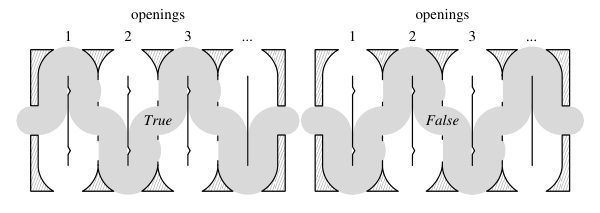
As the last step of the reduction, we convert $I$ to an instance of finding a thick wire. For that, we thicken the edges of $I$, turning them into channels of width 2. We replace variables and clauses with gadgets shown in Figs. 8 and 9 resp. The connections (channels) between variables and clauses (Fig. 10) ensure that whenever a channel from a clause to a variable is used by the wire, the variable satisfies the clause.

We cut (the channel corresponding to) one of the edges of $\mathbb{C}$, and place the points $s,f$ on the opposite sides of the cut. This turns the closed walk $\mathcal{W}$ into an $s\textrm{-}f$ path. By our construction, the only $s\textrm{-}f$ wire in the instance is one that follows the walk $\mathcal{W}$ in $I$, possibly, omitting some clause-variable edges (channels). Indeed, neither channels nor gadgets have any leakage – the wire must follow them through. The only flexibility that the wire has is (1) how to traverse the variable gadgets, and (2) which clause-variable channels (not) to use. But we know, by clause gadget construction (see Fig. 9), that at least one channel from every clause must be used; moreover, when it is used, the variable must satisfy the clause (see Fig. 10). Thus, the $s\textrm{-}f$ wire exists if and only if $I$ is satisfiable.

References

- [1] P. K. Agarwal, A. Efrat, and M. Sharir. Vertical decomposition of shallow levels in 3-dimensional arrangements and its applications. SIAM Journal on Computing, 29(3):912–953, 2000.
- [2] P. K. Agarwal and M. Sharir. Efficient algorithms for geometric optimization. ACM Computing Surveys, 30:412–458, 1998.
- [3] R. Alterovitz, M. S. Branicky, and K. Y. Goldberg. Motion planning under uncertainty for image-guided medical needle steering. International Journal of Robotic Research, 27(11-12):1361–1374, 2008.
- [4] E. M. Arkin, J. S. B. Mitchell, and V. Polishchuk. Maximum thick paths in static and dynamic environments. Computational Geometry Theory and Applications, 43(3):279–294, 2010.
- [5] T. Asano, D. Kirkpatrick, and C. K. Yap. -optimal motion for a rod. In Proceedings of the 12th Annual ACM Symposium on Computational Geometry, pages 252–263, 1996.
- [6] T. Asano, D. Kirkpatrick, and C. K. Yap. Minimizing the trace length of a rod endpoint in the presence of polygonal obstacles is NP-hard. In Proceeding of Canadian Conference on Computational Geometry, pages 10–13, 2003.
- [7] J. Barcia, J. Diaz-Banez, F. Gomez, and I. Ventura. The anchored Voronoi diagram: static and dynamic versions and applications. In 19th European Workshop on Computational Geometry, 2003.
- [8] S. Bereg and D. Kirkpatrick. Curvature-bounded traversals of narrow corridors. In Proceedings of the 21st Annual Symposium on Computational geometry, pages 278–287, 2005.
- [9] L. P. Chew. Planning the shortest path for a disc in time. In Proceedings of the 1st Annual Symposium on Computational Geometry, pages 214–220, 1985.
- [10] D. Chowdhury. Molecular motors: Design, mechanism, and control. Computing in Science and Engineering, 10:70–77, 2008.
- [11] A. F. Cook IV, C. Wenk, O. Daescu, S. Bitner, Y. K. Cheung, and A. Kurdia. Visiting a sequence of points with a bevel-tip needle. In Proceedings of the 9th Latin American Theoretical Informatics Symposium, 2010.
- [12] A. Efrat and M. Sharir. A near-linear algorithm for the planar segment center problem. Discrete & Computational Geometry, 16:239–257, 1996.
- [13] T. Hu, A. Kahng, and G. Robins. Optimal robust path planning in general environments. IEEE Transactions on Robotics and Automation, 9:775–784, 1993.
- [14] I. Kostitsyna and V. Polishchuk. Simple wriggling is hard unless you are a fat hippo. In Fifth International Conference on Fun with Algorithms (FUN), 2010. To appear.
- [15] J.-C. Latombe. Robot Motion Planning. Kluwer, Boston, 1991.
- [16] S. M. LaValle. Planning Algorithms. Cambridge University Press, 2006.
- [17] J. Y. Lee and H. Choset. Sensor-based planning for a rod-shaped robot in three dimensions: Piecewise retracts of R3 x S2. International Journal of Robotic Research, 24(5):343–383, 2005.
- [18] D. Lichtenstein. Planar formulae and their uses. SIAM Journal on Computing, 11(2):329–343, 1982.
- [19] F. M. Maley. Single-Layer Wire Routing and Compaction. MIT Press, 1990.
- [20] K. McEvoy and J. V. Tucker, editors. Theoretical Foundations of VLSI Design. Cambridge University Press, New York, NY, USA, 1991.
- [21] J. Pach and G. Tardos. Forbidden patterns and unit distances. In Proceedings of the 21st Annual Symposium on Computational Geometry, pages 1–9, 2005.
- [22] S. Sifrony and M. Sharir. A new efficient motion-planning algorithm for a rod in two-dimensional polygonal space. Algorithmica, 2:367–402, 1987.
- [23] C. Veigel, L. M. Coluccio, J. D. Jontes, J. C. Sparrow, R. A. Milligan, and J. Molloy. The motor protein myosin-I produces its working stroke in two steps. Nature, 398:530––533, 1999.