$W$ polarisation beyond helicity fractions
in top quark decays

It is generally believed that the study of the top quark, which is singled out among the other fermions by its large mass and short lifetime, will be useful to probe new physics above the electroweak scale [1, 2, 3, 4]. For this reason, top physics constitutes one of the main programs for Tevatron and the Large Hadron Collider (LHC). Apart from determining the top quark quantum numbers to establish that the top quark is indeed what we expect, its mass and couplings will be measured. The former is an input parameter in the Lagrangian, whose precise determination is fundamental to reduce theoretical uncertainties in many observables. On the other hand, top couplings offer an interesting window to new physics. If new particles exist above the electroweak scale, their effect at energies below the resonance thresholds can be parameterised by effective operators [5, 6, 7] invariant under the standard model (SM) gauge symmetry $\text{SU}(3)_{c}\times\text{SU}(2)_{L}\times\text{U}(1)_{Y}$. In the case of top quark couplings, the contribution from these operators is expected to be more important than for the other fermions, due precisely to the large top mass. A general (and minimal) parameterisation of top quark couplings arising from dimension-six effective operators was given in Refs. [8].

Among the different top couplings to the gauge and Higgs bosons, the $Wtb$ vertex deserves a special attention, precisely because the top quark is expected to decay almost exclusively via this interaction, $t\to Wb$. Within the effective operator framework, this vertex can be written in full generality as

	$\displaystyle\mathcal{L}_{Wtb}$	$\displaystyle=$	$\displaystyle-\frac{g}{\sqrt{2}}\bar{b}\,\gamma^{\mu}\left(V_{L}P_{L}+V_{R}P_{R}\right)t\;W_{\mu}^{-}$		(1)
			$\displaystyle-\frac{g}{\sqrt{2}}\bar{b}\,\frac{i\sigma^{\mu\nu}q_{\nu}}{M_{W}}\left(g_{L}P_{L}+g_{R}P_{R}\right)t\;W_{\mu}^{-}+\mathrm{h.c.}$

This Lagrangian is assumed to be Hermitian in order to preserve unitarity, as it is demanded for a fundamental theory of elementary particle interactions, from which effective operators arise by integration of the heavy degrees of freedom. This implies that all complex phases in our effective Lagrangian are CP violating. We will not introduce any of the so-called “CP-conserving phases” [9, 10, 11] since they lead to a non-Hermitian Lagrangian with some undesired effects.¹¹ 1 Such phases could appear in the $t\to Wb$ decay amplitude from unitarity corrections, associated with the absorptive parts of higher-order diagrams involving new states lighter than the top quark. The presence of such states, however, contradicts the spirit of the effective operator framework, where new physics is assumed to be heavy, and invariant under the (unbroken) SM gauge group.

In the SM, the $Wtb$ vertex in Eq. (1) reduces to $V_{L}=V_{tb}\simeq 1$ and $V_{R}=g_{L}=g_{R}=0$ at the tree level. Deviations from these values (see for example Refs. [12, 13, 14, 15, 16, 17]) can be tested by measuring various observables. In particular, the presence of non-zero anomalous couplings $V_{R}$, $g_{L}$, $g_{R}$ is probed with good precision by determining the helicity of the $W$ boson in the top quark decay, i.e. the relative fractions $F_{+}$, $F_{0}$, $F_{-}$ of $W$ bosons produced with helicity $+1$, $0$, $-1$ [18], and through angular distributions in the top quark rest frame [19, 20]. Still, these observables do not contain all the information from the top decay, in particular regarding complex phases. As we will show in this paper, the density matrix for a polarised top quark decay is determined by eight form factors which are functions of the $Wtb$ couplings in Eq. (1). Three of these factors appear in the helicity fractions, while the five remaining ones do not. We will find that a simple and convenient way to probe some of them is by measuring the transverse and normal $W$ polarisation fractions $F_{\pm,0}^{T}$, $F_{\pm,0}^{N}$. These are the probabilities for having definite spin components along two directions (transverse and normal) orthogonal to the $W$ momentum. The normal $W$ polarisation deserves a special mention. A net normal polarisation ($F^{N}_{+}\neq F^{N}_{-}$) unambiguously signals the presence of complex phases in the $Wtb$ vertex because it is directly proportional to the imaginary part of products of $Wtb$ couplings. On the other hand, helicity fractions and distributions in the top quark rest frame involve the real parts of products and moduli squared. Complex phases can also be probed through triple-product asymmetries in $t\bar{t}$ production, involving decay products of both $t$ and $\bar{t}$ [21, 22, 9, 10, 11] but, in contrast, the normal $W$ polarisation can be studied for $t$ (or $\bar{t}$) decays independently. The power of observables like the transverse and normal polarisations for the study of new physics couplings has been demonstrated for $\tau$ leptons at the $Z$ peak [23, 24] and at $B$ factories [25, 26].

The measurement of $W$ transverse and normal polarisation fractions requires the production of polarised top quarks, so that the transverse and normal directions, defined within and orthogonal to the plane determined by the $W$ momentum and the top polarisation, are meaningful. This will take place, for example, in $t$-channel single top production at LHC, in which the top quarks will have a large polarisation in the direction of the spectator jet [27]. The determination of $W$ polarisation fractions in this process is expected to achieve a good accuracy, due to the good statistics for this process. In this paper we will show that the measurement of the transverse and normal polarisation fractions (or related observables) will allow to perform a model-independent determination of the complex $Wtb$ vertex in Eq. (1), also using helicity fractions, asymmetries in the top quark rest frame and the $tW$ total cross section. A bonus from this analysis is that the single top polarisation, which is taken as a free parameter, can be obtained in a model-independent way from the fit, i.e. without assumptions on the $Wtb$ couplings. Our fits will be performed with an upgraded version 2 of the TopFit package,²² 2 The code can be downloaded from http://www-ftae.ugr.es/topfit. extended to include many new observables as well as complex anomalous couplings.

We emphasise that a model-independent determination of the $Wtb$ vertex will be important even if it does not lead to new physics discoveries. Even if new physics does not contribute sizeably to the $Wtb$ vertex and the top quark decays as predicted by the SM, it is crucial to establish this fact in a model-independent way, in order to clearly identify possible new physics in top quark production, if present. One interesting example of this interplay concerns the production of top quark pairs at LHC. Their polarisation (which is very small in the SM) and spin correlation may be modified by the presence of new production mechanisms [28, 29, 30], and hence they probe new physics in $t\bar{t}$ production. However, the (anti)top polarisation and top-antitop spin correlation can only be measured through angular distributions of $t$, $\bar{t}$ decay products, which are also sensitive to $Wtb$ anomalous couplings. Performing model-independent measurements of the former obviously requires that the $Wtb$ vertex is precisely measured and possible anomalous couplings are bound. Analogously, in $t$-channel single top production the top polarisation probes new mechanisms for the production, as for example four-fermion operators, new charged gauge bosons and top flavour-changing neutral couplings [31, 32, 33]. In this case, a model-independent determination of the single top polarisation (as the one obtained from our fit) is welcome.

The structure of this paper is the following. In the next section we write down the density matrix for polarised (anti)top decays in the helicity basis using the $Wtb$ vertex in Eq. (1). In section 3 we introduce the transverse and normal polarisation fractions, give their expressions, examine their dependence on anomalous couplings and discuss their experimental measurement from angular distributions. Related observables, such as asymmetries in these angular distributions, are defined and studied in section 4. In particular, a T-odd forward-backward asymmetry, very sensitive to the phase of $g_{R}$, is introduced and compared with triple product asymmetries in $t\bar{t}$ decays. Present and future limits on the transverse and normal polarisation fractions are examined in sections 5 and 6, showing that their measurement will bring new information about the $Wtb$ vertex. In section 7 we present our model-independent fit to the $Wtb$ vertex using estimations for the expected LHC sensitivities of the different observables. The resulting constraints are used in section 8 to determine the possible contributions of new physics to the decay vertex and their implications for spin correlations in $t\bar{t}$ production at LHC. Finally, in section 9 we adopt the opposite approach: we consider that only one anomalous coupling is non-zero and study the deviations which would show up in the most sensitive observables. We summarise our results in section 10. The vector boson polarisation vectors used in our calculations and the relations among them are given in the appendix.

The polarisation of the $W$ bosons produced in the top decay is sensitive to non-standard $Wtb$ couplings [18]. We calculate here the density matrix for the decay of a polarised top quark into a polarised $W$ boson and a massive $b$ quark. (See Ref. [34] for an early calculation within the SM.) The program FORM [35] is used for the symbolic manipulations. For the $W$ boson spin we use the helicity basis (see the appendix) choosing the positive $z$ axis in the direction of its momentum in the top quark rest frame $\vec{q}$. The top spin direction is parameterised as

$$s_{t}=(0,\sin\theta\cos\phi,\sin\theta\sin\phi,\cos\theta)\,.$$

(2)

The spin density matrix elements for $W$ helicity components $i,j=0,\pm 1$ are

$$\mathcal{A}(t\to W_{i}b)\,\mathcal{A}^{*}(t\to W_{j}b)=\frac{g^{2}}{4}m_{t}^{2}M_{ij}\,,$$

(3)

being

		$\displaystyle M_{00}=A_{0}+2\frac{|\vec{q}\,|}{m_{t}}A_{1}\cos\theta\,,$
		$\displaystyle M_{++}=B_{0}\,(1+\cos\theta)+2\frac{|\vec{q}\,|}{m_{t}}B_{1}\,(1+\cos\theta)\,,$
		$\displaystyle M_{--}=B_{0}\,(1-\cos\theta)-2\frac{|\vec{q}\,|}{m_{t}}B_{1}\,(1-\cos\theta)\,,$
		$\displaystyle M_{0+}=M_{+0}^{*}=\left[\frac{m_{t}}{\sqrt{2}M_{W}}(C_{0}-iD_{0})+\frac{|\vec{q}\,|}{\sqrt{2}M_{W}}(C_{1}-iD_{1})\right]\sin\theta e^{i\phi}\,,$
		$\displaystyle M_{0-}=M_{-0}^{*}=\left[\frac{m_{t}}{\sqrt{2}M_{W}}(C_{0}-iD_{0})-\frac{|\vec{q}\,|}{\sqrt{2}M_{W}}(C_{1}-iD_{1})\right]\sin\theta e^{-i\phi}\,,$
		$\displaystyle M_{+-}=M_{-+}=0\,.$		(4)

The dependence on the $Wtb$ couplings in Eq. (1) is encoded in eight dimensionless form factors

	$\displaystyle A_{0}$	$\displaystyle=\frac{m_{t}^{2}}{M_{W}^{2}}\left[|V_{L}|^{2}+|V_{R}|^{2}\right]\left(1-x_{W}^{2}\right)+\left[|g_{L}|^{2}+|g_{R}|^{2}\right]\left(1-x_{W}^{2}\right)$
		$\displaystyle-4x_{b}\,\text{Re}\,\left[V_{L}V_{R}^{*}+g_{L}g_{R}^{*}\right]-2\frac{m_{t}}{M_{W}}\text{Re}\,\,\left[V_{L}g_{R}^{*}+V_{R}g_{L}^{*}\right]\left(1-x_{W}^{2}\right)$
		$\displaystyle+2\frac{m_{t}}{M_{W}}x_{b}\,\text{Re}\,\,\left[V_{L}g_{L}^{*}+V_{R}g_{R}^{*}\right]\left(1+x_{W}^{2}\right)\,,$
	$\displaystyle A_{1}$	$\displaystyle=\frac{m_{t}^{2}}{M_{W}^{2}}\left[|V_{L}|^{2}-|V_{R}|^{2}\right]-\left[|g_{L}|^{2}-|g_{R}|^{2}\right]-2\frac{m_{t}}{M_{W}}\text{Re}\,\,\left[V_{L}g_{R}^{*}-V_{R}g_{L}^{*}\right]$
		$\displaystyle+2\frac{m_{t}}{M_{W}}x_{b}\text{Re}\,\,\left[V_{L}g_{L}^{*}-V_{R}g_{R}^{*}\right]\,,$
	$\displaystyle B_{0}$	$\displaystyle=\left[|V_{L}|^{2}+|V_{R}|^{2}\right]\left(1-x_{W}^{2}\right)+\frac{m_{t}^{2}}{M_{W}^{2}}\left[|g_{L}|^{2}+|g_{R}|^{2}\right]\left(1-x_{W}^{2}\right)$
		$\displaystyle-4x_{b}\,\text{Re}\,\left[V_{L}V_{R}^{*}+g_{L}g_{R}^{*}\right]-2\frac{m_{t}}{M_{W}}\text{Re}\,\,\left[V_{L}g_{R}^{*}+V_{R}g_{L}^{*}\right]\left(1-x_{W}^{2}\right)$
		$\displaystyle+2\frac{m_{t}}{M_{W}}x_{b}\,\text{Re}\,\,\left[V_{L}g_{L}^{*}+V_{R}g_{R}^{*}\right]\left(1+x_{W}^{2}\right)\,,$
	$\displaystyle B_{1}$	$\displaystyle=-\left[|V_{L}|^{2}-|V_{R}|^{2}\right]+\frac{m_{t}^{2}}{M_{W}^{2}}\left[|g_{L}|^{2}-|g_{R}|^{2}\right]+2\frac{m_{t}}{M_{W}}\,\text{Re}\,\,\left[V_{L}g_{R}^{*}-V_{R}g_{L}^{*}\right]$
		$\displaystyle+2\frac{m_{t}}{M_{W}}x_{b}\,\text{Re}\,\,\left[V_{L}g_{L}^{*}-V_{R}g_{R}^{*}\right]\,,$
	$\displaystyle C_{0}$	$\displaystyle=\left[|V_{L}|^{2}+|V_{R}|^{2}+|g_{L}|^{2}+|g_{R}|^{2}\right]\left(1-x_{W}^{2}\right)-2x_{b}\,\text{Re}\,\left[V_{L}V_{R}^{*}+g_{L}g_{R}^{*}\right]\left(1+x_{W}^{2}\right)$
		$\displaystyle-\frac{m_{t}}{M_{W}}\text{Re}\,\,\left[V_{L}g_{R}^{*}+V_{R}g_{L}^{*}\right]\left(1-x_{W}^{4}\right)+4x_{W}x_{b}\,\text{Re}\,\,\left[V_{L}g_{L}^{*}+V_{R}g_{R}^{*}\right]\,,$
	$\displaystyle C_{1}$	$\displaystyle=2\left[-|V_{L}|^{2}+|V_{R}|^{2}+|g_{L}|^{2}-|g_{R}|^{2}\right]+2\frac{m_{t}}{M_{W}}\text{Re}\,\,\left[V_{L}g_{R}^{*}-V_{R}g_{L}^{*}\right]\left(1+x_{W}^{2}\right)\,,$
	$\displaystyle D_{0}$	$\displaystyle=\frac{m_{t}}{M_{W}}\text{Im}\,\,\left[V_{L}g_{R}^{*}+V_{R}g_{L}^{*}\right]\left(1-2x_{W}^{2}+x_{W}^{4}\right)\,,$
	$\displaystyle D_{1}$	$\displaystyle=-4x_{b}\,\text{Im}\,\left[V_{L}V_{R}^{*}+g_{L}g_{R}^{*}\right]-2\frac{m_{t}}{M_{W}}\text{Im}\,\left[V_{L}g_{R}^{*}-V_{R}g_{L}^{*}\right](1-x_{W}^{2})\,,$		(5)

with $x_{W}=M_{W}/m_{t}$, $x_{b}=m_{b}/m_{t}$. The $W$ momentum in the top quark rest frame is

$$|\vec{q}\,|=\frac{m_{t}}{2}(1-x_{W}^{2})\,.$$

(6)

We emphasise that, while in the SM it is safe to neglect the $b$ quark mass [18, 36], in the presence of the anomalous couplings $V_{R}$ and $g_{L}$ this is no longer possible [37, 38]. Indeed, linear interference terms like $x_{b}\,V_{L}g_{L}^{*}$ and $x_{b}\,V_{L}V_{R}^{*}$ can be of the same size as the quadratic ones $|g_{L}|^{2}$, $|V_{R}|^{2}$ for $g_{L}$ and $V_{R}$ small. On the other hand, in the above expressions we have omitted terms of order $x_{b}^{2}$ and higher, which amount to corrections of the order of $10^{-3}$ or smaller. All terms are kept in our numerical code, however. The best sensitivity is expected for both $\text{Re}\,g_{R}$ and $\text{Im}\,g_{R}$, due to their interference with $V_{L}$ without any suppression by $x_{b}$. It is also worthwhile to remark here that $D_{0}$, $D_{1}$ are proportional to the imaginary parts of products of $Wtb$ couplings, in contrast with the other terms which contain the moduli squared and the real parts. The form factors $D_{0}$, $D_{1}$ are thus entirely new physics effects. The spin density matrix elements $\bar{M}_{ij}$ for antitop decays are

		$\displaystyle\bar{M}_{00}=A_{0}-2\frac{|\vec{q}\,|}{m_{t}}A_{1}\cos\theta\,,$
		$\displaystyle\bar{M}_{++}=B_{0}\,(1+\cos\theta)-2\frac{|\vec{q}\,|}{m_{t}}B_{1}\,(1+\cos\theta)\,,$
		$\displaystyle\bar{M}_{--}=B_{0}\,(1-\cos\theta)+2\frac{|\vec{q}\,|}{m_{t}}B_{1}\,(1-\cos\theta)\,,$
		$\displaystyle\bar{M}_{0+}=\bar{M}_{+0}^{*}=\left[\frac{m_{t}}{\sqrt{2}M_{W}}(C_{0}+iD_{0})-\frac{|\vec{q}\,|}{\sqrt{2}M_{W}}(C_{1}+iD_{1})\right]\sin\theta e^{i\phi}\,,$
		$\displaystyle\bar{M}_{0-}=\bar{M}_{-0}^{*}=\left[\frac{m_{t}}{\sqrt{2}M_{W}}(C_{0}+iD_{0})+\frac{|\vec{q}\,|}{\sqrt{2}M_{W}}(C_{1}+iD_{1})\right]\sin\theta e^{-i\phi}\,,$
		$\displaystyle\bar{M}_{+-}=\bar{M}_{-+}=0\,.$		(7)

The partial widths for the top decay into a $W$ boson with $+1$, $0$ or $-1$ helicity, denoted here as $\Gamma_{+}$, $\Gamma_{0}$, $\Gamma_{-}$ respectively, can be straightforwardly obtained from Eqs. (4), (5) by integrating over $\cos\theta$, $\phi$ and including the appropriate phase space factors. They are [38]

$\displaystyle\Gamma_{0}=\frac{g^{2}|\vec{q}\,|}{32\pi}A_{0}\,,$

$\displaystyle\Gamma_{\pm}=\frac{g^{2}|\vec{q}\,|}{32\pi}\left(B_{0}\pm 2\frac{|\vec{q}\,|}{m_{t}}B_{1}\right)\,.$

(8)

Since the total width $\Gamma(t\to Wb)=\Gamma_{-}+\Gamma_{0}+\Gamma_{+}$ is about 8 times smaller than the expected width of the top invariant mass peak [39, 40], measuring deviations in $\Gamma$ due to anomalous couplings or $V_{L}$ different from one seems rather difficult. Instead, the $W$ helicity fractions $F_{i}\equiv\Gamma_{i}/\Gamma$ are usually studied. At the tree level, $F_{-}=0.2971$, $F_{0}=0.7025$, $F_{+}=0.000359$ in the SM for $m_{t}=175$ GeV, $M_{W}=80.4$ GeV, $m_{b}=4.8$ GeV. At NNLO in QCD, $F_{-}=0.311$, $F_{0}=0.687$, $F_{+}=0.0017$ [41] for a slightly smaller value of the top quark mass $m_{t}=172.8$ GeV.

Helicity fractions can be measured in leptonic decays $W\to\ell\nu$. Let us denote by $\theta_{\ell}^{*}$ the angle between the charged lepton three-momentum in the $W$ rest frame and the $W$ momentum in the $t$ rest frame (corresponding to the spin axis in the helicity basis). Then, the normalised angular distribution of the charged lepton is given by

$$\frac{1}{\Gamma}\frac{d\Gamma}{d\!\cos\theta_{\ell}^{*}}=\frac{3}{8}(1+\cos\theta_{\ell}^{*})^{2}\,F_{+}+\frac{3}{8}(1-\cos\theta_{\ell}^{*})^{2}\,F_{-}+\frac{3}{4}\sin^{2}\theta_{\ell}^{*}\,F_{0}\,,$$

(9)

with the three terms corresponding to the three helicity states.³³ 3 Note that the off-diagonal terms of the spin density matrix give vanishing integral, which implies that $\sum_{i}|\mathcal{A}(t\to W_{i}b\to\ell\nu)|^{2}\propto\sum_{i}|\mathcal{A}(t\to W_{i}b)|^{2}\times|\mathcal{A}(W_{i}\to\ell\nu)|^{2}$ in the narrow width approximation and justifies the use of Eq. (9) for this basis. Moreover, the off-diagonal terms in the $W\to\ell\nu$ density matrix vanish when integrated on the azimuthal angle with respect to the $W$ spin quantisation axis, which also justifies this decomposition for any basis. A fit to the $\cos\theta_{\ell}^{*}$ distribution allows to extract from experiment the values of $F_{i}$, which are not independent but satisfy $F_{+}+F_{-}+F_{0}=1$ by definition.

For unpolarised top quark decays, the only meaningful direction in the top quark rest frame is the one of the $W$ boson (and $b$ quark) three-momentum. However, for polarised top quark decays further spin directions may be considered, as indicated in Fig. 1:

• (i)

  the transverse direction $\vec{T}$, defined as the axis orthogonal to the $W$ momentum $\vec{q}$ and contained in the plane defined by it and the top quark spin direction $\vec{s}_{t}$,

• (ii)

  the normal direction $\vec{N}$, perpendicular to the plane defined by the $W$ momentum and the top spin direction.

We define the transverse and normal vectors as

		$\displaystyle\vec{N}=\vec{s}_{t}\times\vec{q}\,,$
		$\displaystyle\vec{T}=\vec{q}\times\vec{N}\,,$		(10)

corresponding to the ones shown in the figure. For these two spin directions, two further sets of polarised $W$ partial widths can be defined, $\Gamma^{T}_{-}$, $\Gamma^{T}_{0}$, $\Gamma^{T}_{+}$ (transverse) and $\Gamma^{N}_{-}$, $\Gamma^{N}_{0}$, $\Gamma^{N}_{+}$ (normal). They can be obtained either (i) by direct computation using the polarisation vectors given in the appendix, or (ii) by using their relation with the helicity basis and the spin density matrix elements for $\phi=\pi/2$. We have performed both calculations as a cross-check. The polarised partial widths for a general $Wtb$ vertex are

		$\displaystyle\Gamma^{T}_{0}=\Gamma^{N}_{0}=\frac{g^{2}|\vec{q}\,|}{32\pi}B_{0}\,,$		$\displaystyle\Gamma^{T}_{\pm}=\frac{g^{2}|\vec{q}\,|}{32\pi}\left(\frac{A_{0}+B_{0}}{2}\pm\frac{\pi}{4}\frac{m_{t}}{M_{W}}C_{0}\right)\,,$
		$\displaystyle\Gamma^{N}_{\pm}=\frac{g^{2}|\vec{q}\,|}{32\pi}\left(\frac{A_{0}+B_{0}}{2}\pm\frac{\pi}{4}\frac{|\vec{q}\,|}{M_{W}}D_{1}\right)\,.$				(11)

These quantities are very useful to access some of the off-diagonal terms in the spin density matrix, namely $C_{0}$ and $D_{1}$. We point out that $\Gamma^{N}_{-}=\Gamma^{N}_{+}$ if CP is conserved in the $Wtb$ vertex, i.e. if all anomalous couplings are real ($V_{L}$ can always be made real with a redefinition of the quark fields). This implies that a net normal $W$ polarisation ($\Gamma^{N}_{-}\neq\Gamma^{N}_{+}$) can only be produced if CP is violated in the $t\to Wb$ decay.⁴⁴ 4 We note that the normal polarisation $\Gamma^{N}_{+}-\Gamma^{N}_{-}$ is T-odd but not a genuine CP-violating observable, if absorptive parts were present in the decay amplitude. This property is unique to the normal direction. Although the helicity and transverse polarisation (as well as top rest frame distributions, see section 6) obviously depend quadratically on the imaginary part of anomalous couplings through the moduli squared, their measurement cannot clearly signal the presence of complex phases in the $Wtb$ vertex as the normal polarisation can, through the linear interference term $\text{Im}\,V_{L}g_{R}^{*}$.

The transverse and normal polarisation fractions $F_{i}^{T}$, $F_{i}^{N}$ are defined by normalising to the total width for $t\to Wb$. It is very interesting to observe that they obey a sum rule,

$$F^{T}_{0}=F^{N}_{0}=\frac{1}{2}(F_{+}+F_{-})\,,$$

(12)

which can be obtained either from the explicit expressions of the partial widths or by using the relations among polarisation vectors and the fact that $M_{+-}=0$. Additionally, for a real $Wtb$ vertex,

$$F^{N}_{+}=F^{N}_{-}=\frac{1}{2}-\frac{1}{4}(F_{+}+F_{-})\,.$$

(13)

These equations constrain the possible variation of transverse and normal polarisation fractions once that the helicity fractions are measured (see section 5). Their tree-level values in the SM are $F^{T}_{-}=0.1718$, $F^{T}_{0}=0.1487$, $F^{T}_{+}=0.6794$, and $F^{N}_{-}=0.4256$, $F^{N}_{0}=0.1487$, $F^{N}_{+}=0.4256$. For illustration, we show in Figs. 2 and 3 the variation of all polarisation fractions for small values of the anomalous couplings, considering only one non-zero anomalous coupling at a time and setting $V_{L}=1$ as in the SM. We plot the dependence on the real part of anomalous couplings in Fig. 2, whereas the dependence on the imaginary parts is displayed in Fig. 3.

Comparing both sets of plots we observe that helicity and transverse polarisation fractions are much more sensitive to $\text{Re}\,g_{R}$ than to $\text{Im}\,g_{R}$, while $F^{N}_{\pm}$ are also very sensitive to $\text{Im}\,g_{R}$. Thus, we can anticipate that the eventual measurement of normal $W$ polarisation fractions will significantly improve the constraints on the latter. For a given observable, it is also seen that the dependence on the real and imaginary parts of $V_{R}$ is similar (but different from one observable to another). The same comment also applies to $g_{L}$.

As the helicity fractions, the transverse and normal polarisation fractions can be measured in top semileptonic decays. We define the angles $\theta_{\ell}^{T}$ ($\theta_{\ell}^{N}$) between the charged lepton momentum in the $W$ rest frame and the transverse (normal) directions in the top quark rest frame, given by Eqs. (10). Then, the charged lepton distribution has the same form as for the angle $\theta_{\ell}^{*}$ in the helicity basis,

$$\frac{1}{\Gamma}\frac{d\Gamma}{d\!\cos\theta_{\ell}^{T,N}}=\frac{3}{8}(1+\cos\theta_{\ell}^{T,N})^{2}\,F^{T,N}_{+}+\frac{3}{8}(1-\cos\theta_{\ell}^{T,N})^{2}\,F^{T,N}_{-}+\frac{3}{4}\sin^{2}\theta_{\ell}^{T,N}\,F^{T,N}_{0}\,.$$

(14)

The three $\cos\theta_{\ell}^{*}$, $\cos\theta_{\ell}^{T}$, $\cos\theta_{\ell}^{N}$ distributions are presented in Fig. 4 for the SM.

However, in most processes the top quarks are not produced with 100% polarisation along any axis, but with a certain degree of polarisation

$$P=\frac{N_{\uparrow}-N_{\downarrow}}{N_{\uparrow}+N_{\downarrow}}\,.$$

(15)

In this case, the distributions are obtained by substituting in Eq. (14) the $W$ polarisation fractions by the “effective” quantities

		$\displaystyle\tilde{F}^{T,N}_{+}=\left[\frac{1+P}{2}F^{T,N}_{+}+\frac{1-P}{2}F^{T,N}_{-}\right]\,,$
		$\displaystyle\tilde{F}^{T,N}_{-}=\left[\frac{1+P}{2}F^{T,N}_{-}+\frac{1-P}{2}F^{T,N}_{+}\right]\,,$
		$\displaystyle\tilde{F}^{T,N}_{0}=F^{T,N}_{0}\,,$		(16)

which are the ones actually measured. Notice that $F^{T,N}_{0}$ is unchanged. For an unpolarised top quark ($P=0$) the resulting distributions are symmetric ($\tilde{F}^{T,N}_{+}=\tilde{F}^{T,N}_{-}$) as one may expect from symmetry arguments. However, the distributions are not isotropic ($\tilde{F}^{T,N}_{\pm}\neq\tilde{F}^{T,N}_{0}$) because there is still a privileged direction in space, the $W$ boson momentum. Experimentally, these distributions can be measured as follows:

1. 1.

   In the top quark rest frame, the normal and transverse directions are obtained from Eqs. (10) using for $\vec{s}_{t}$ some spatial direction, preferrably one in which the top quark is produced with a large polarisation (e.g. the spectator jet momentum in the top rest frame, for $t$-channel single top production [27]).

2. 2.

   The momentum of the charged lepton in the $W$ rest frame is obtained performing a boost on its momentum in the top quark rest frame.

3. 3.

   The angles $\theta_{\ell}^{T}$, $\theta_{\ell}^{N}$ correspond to the ones between the charged lepton and the two directions previously determined.

We have checked our analytical results for the $W$ polarisation fractions by comparing the predicted distributions with tree-level Monte Carlo calculations in $t$-channel single top production using Protos [42] and different values of the anomalous couplings, obtaining very good agreement between them.

We conclude this section with a discussion of the corresponding observables for $\bar{t}\to W^{-}\bar{b}$ decays. By explicit calculation it is found that the $W$ polarisation fractions for this decay (denoted with a bar) satisfy

		$\displaystyle\bar{F}_{0}=F_{0}\,,\quad\bar{F}_{\pm}=F_{\mp}\,,$
		$\displaystyle\bar{F}_{0}^{T}=F_{0}^{T}\,,\quad\bar{F}_{\pm}^{T}=F_{\pm}^{T}\,,$
		$\displaystyle\bar{F}_{0}^{N}=F_{0}^{N}\,,\quad\bar{F}_{\pm}^{N}=F_{\pm}^{N}$		(17)

in full generality, even if the $Wtb$ vertex is CP violating. It is very interesting to observe that CP conservation implies

		$\displaystyle\bar{F}_{0}=F_{0}\,,\quad\bar{F}_{\pm}=F_{\mp}\,,$
		$\displaystyle\bar{F}_{0}^{T}=F_{0}^{T}\,,\quad\bar{F}_{\pm}^{T}=F_{\pm}^{T}\,,$
		$\displaystyle\bar{F}_{0}^{N}=F_{0}^{N}\,,\quad\bar{F}_{\pm}^{N}=F_{\mp}^{N}\,.$		(18)

Then, as expected the longitudinal and transverse polarisation fractions cannot give any information on possible CP-violating effects. On the other hand, for the normal polarisation fractions the simultaneous fulfilment of Eqs. (17) and (18) implies $F_{+}^{N}=F_{-}^{N}$, as is the case for a CP-conserving $Wtb$ vertex. These relations among polarisation fractions imply that:

• (i)

  The $\cos\theta_{\ell}^{*}$ distributions are the same for $t$ and $\bar{t}$ decays because, although the helicity fractions are interchanged, $\bar{F}_{\pm}=F_{\mp}$, the $\cos\theta$ terms in Eqs. (9) and (14) also change their sign for $W^{-}$ decays.

• (ii)

  For the same reason, the $\cos\theta_{\ell}^{T}$ and $\cos\theta_{\ell}^{N}$ distributions are also the same provided that the antitop polarisation is the opposite as the one for the top for the axis chosen, $P_{\bar{t}}=-P_{t}$.

The introduction of the transverse and normal polarisation fractions and the $\cos\theta_{\ell}^{T}$, $\cos\theta_{\ell}^{N}$ distributions opens the possibility of new angular asymmetries in top quark decays, in complete analogy with the ones obtained for the $\cos\theta_{\ell}^{*}$ distribution [38]. One can define asymmetries around any fixed point $z$ in the interval $[-1,1]$,

$$A_{z}=\frac{N(\cos\theta>z)-N(\cos\theta<z)}{N(\cos\theta>z)+N(\cos\theta<z)}\,,$$

(19)

for $\theta=\theta_{\ell}^{*},\theta_{\ell}^{T},\theta_{\ell}^{N}$. The most obvious choice is $z=0$, giving forward-backward (FB) asymmetries

		$\displaystyle A_{\text{FB}}=\frac{3}{4}[F_{+}-F_{-}]\,,$
		$\displaystyle A_{\text{FB}}^{T,N}=\frac{3}{4}[\tilde{F}^{T,N}_{+}-\tilde{F}^{T,N}_{-}]=\frac{3}{4}P[F^{T,N}_{+}-F^{T,N}_{-}]\,.$		(20)

The FB asymmetry in the $\cos\theta_{\ell}^{*}$ distribution $A_{\text{FB}}$ [43, 44] does not depend on the top polarisation, while the two other ones are proportional to $P$. Their more relevant dependence on anomalous couplings is shown in Fig. 5.

The asymmetry $A_{\text{FB}}^{N}$, which vanishes for real anomalous couplings (in particular, within the SM), is very sensitive to $\text{Im}\,g_{R}$, as it can be seen in the right plot of this figure. For small $g_{R}$, taking $V_{L}=1$, $V_{R}=g_{L}=0$, we obtain

$$A_{\text{FB}}^{N}=0.64\,P\,\text{Im}\,g_{R}\,.$$

(21)

The numerical coefficient in this asymmetry has also been verified with the Monte Carlo generator Protos. The dependence on $V_{R}$ is much weaker because it is suppressed by $m_{b}/m_{t}$, and the asymmetry does not depend on $g_{L}$ if the other anomalous couplings vanish. This asymmetry is the same (up to a minus sign) as the one based on the triple product [18]

$$\vec{s}_{t}\cdot(\vec{p}_{b}\times\vec{p}_{\ell})\,,$$

(22)

with the $b$ quark and charged lepton momenta taken in the top quark rest frame. Both asymmetries, although sensitive to CP-violating phases in the top decay vertex, are not genuinely CP violating and could be faked by unitarity phases (not considered in our work). The sum of asymmetries for $t$ and $\bar{t}$ decays,

$$A_{\text{FB}}^{\text{CP}}=A_{\text{FB}}^{N}(t)+A_{\text{FB}}^{N}(\bar{t})$$

(23)

is unambiguously CP violating.

It is worthwhile to remark here that $A_{\text{FB}}^{N}$ can be relatively large because it directly probes the imaginary parts of the off-diagonal density matrix elements for a polarised top quark decay, namely $D_{1}$ in Eqs. (5). Therefore, it is expected to be much larger than CP-violating asymmetries based on triple-product spin correlations in $t\bar{t}$ production [21, 22, 9, 10, 11]. Using Protos for $t\bar{t}$ generation with anomalous $Wtb$ couplings,⁵⁵ 5 This generator has been thoroughly tested, validated and is used for official production of $t\bar{t}$ samples with anomalous $Wtb$ couplings in ATLAS. we actually find CP asymmetries numerically much smaller (up to a factor of 35) than the ones obtained in Ref. [10]. For example,

		$\displaystyle\tilde{A}_{1}=(0.0886\pm 0.0015)\,\text{Im}\,g_{R}=(-0.0407\pm 0.0007)f_{t}\sin\phi_{f}\,,$
		$\displaystyle\tilde{A}_{2}=(0.0191\pm 0.0015)\,\text{Im}\,g_{R}=(-0.0087\pm 0.0007)f_{t}\sin\phi_{f}\,,$
		$\displaystyle\tilde{A}_{3}=(0.0328\pm 0.0015)\,\text{Im}\,g_{R}=(-0.0150\pm 0.0007)f_{t}\sin\phi_{f}\,,$		(24)

where $\tilde{A}_{1-3}$ have been defined in Ref. [10] and $\text{Im}\,g_{R}=-M_{W}/m_{t}f_{t}\sin\phi_{f}$ in their notation. The uncertainties quoted come from the Monte Carlo statistics. The numerical results we obtain for $\tilde{A}_{1-3}$ seem consistent with the expectation that spin correlation asymmetries, in particular the CP-violating ones, are suppressed by the spin correlation between the top and antitop, among other factors. (See Eqs. (39) in section 8 for CP-conserving correlations.)

Other convenient choices for asymmetries in the $\cos\theta$ distributions are $z=\mp(2^{2/3}-1)$. Defining $\beta=2^{1/3}-1$, we have

		$\displaystyle z=-(2^{2/3}-1)$	$\displaystyle\rightarrow\quad$	$\displaystyle A_{+}=3\beta[F_{0}+(1+\beta)F_{+}]\,,$
		$\displaystyle A_{+}^{T,N}=3\beta[F^{T,N}_{0}+(1+\beta)\tilde{F}^{T,N}_{+}]\,,$
		$\displaystyle z=(2^{2/3}-1)$	$\displaystyle\rightarrow\quad$	$\displaystyle A_{-}=-3\beta[F_{0}+(1+\beta)F_{-}]\,,$
		$\displaystyle A_{-}^{T,N}=-3\beta[F^{T,N}_{0}+(1+\beta)\tilde{F}^{T,N}_{-}]\,.$				(25)

The resulting asymmetries only depend on two “effective” polarisation fractions. Conversely, the latter quantities can also be determined from asymmetries, for example

	$\displaystyle\tilde{F}^{T,N}_{+}$	$\displaystyle=$	$\displaystyle\frac{1}{1-\beta}+\frac{A_{-}^{T,N}-\beta A_{+}^{T,N}}{3\beta(1-\beta^{2})}\,,$
	$\displaystyle\tilde{F}^{T,N}_{-}$	$\displaystyle=$	$\displaystyle\frac{1}{1-\beta}-\frac{A_{+}^{T,N}-\beta A_{-}^{T,N}}{3\beta(1-\beta^{2})}\,,$
	$\displaystyle F^{T,N}_{0}$	$\displaystyle=$	$\displaystyle-\frac{1+\beta}{1-\beta}+\frac{A_{+}^{T,N}-A_{-}^{T,N}}{3\beta(1-\beta)}\,.$		(26)

The angular asymmetries $A_{\text{FB}}^{T,N}$, $A_{+}^{T,N}$, $A_{-}^{T,N}$ do not provide any further information than the polarisation fractions $\tilde{F}^{T,N}_{+}$, $\tilde{F}^{T,N}_{-}$, $F^{T,N}_{0}$ do. Still, their measurement may be more convenient from the experimental point of view, especially with low statistics, since it does not require fitting the $\cos\theta_{\ell}^{T,N}$ distributions. Moreover, systematic uncertainties on the asymmetries may be smaller than on the polarisation fractions,⁶⁶ 6 For a detailed comparison of systematic uncertainties on helicity fractions, their ratios and angular asymmetries see Ref. [45]. so that the constraints placed on anomalous $Wtb$ couplings may be stronger. A detailed evaluation of systematic uncertainties for these measurements is compulsory before drawing any conclusion in this respect.

As we have remarked, the sum rule in Eq. (12) implies that the measurement of helicity fractions in top quark decays automatically fixes the $F^{T}_{0}$, $F^{N}_{0}$ components of the transverse and normal $W$ polarisation. Still, the other four components are undetermined in principle. We have investigated their possible range of variation given the present Tevatron measurements [46] and the future expectations for LHC with 10 fb^-1 at a centre of mass (CM) energy of 14 TeV [45]. We take

		$\displaystyle F_{0}=0.88\pm 0.125\,,\quad F_{+}=-0.15\pm 0.0921\,,\quad\text{corr}=-0.59$		$\displaystyle\text{(Tevatron)}\,,$
		$\displaystyle F_{0}=0.700\pm 0.0192\,,\quad F_{+}=0.0006\pm 0.00216$		$\displaystyle\text{(LHC)}\,.$		(27)

For the forthcoming LHC measurements the correlation has not yet been estimated and is therefore ignored. We also use single top cross section measurements, which constrain the anomalous couplings in Eq. (1) and then, indirectly, the $W$ polarisation fractions. For Tevatron we use the combined $s+t$-channel measurement [47] which has a better precision than the separate ones for the $s$- and $t$-channels. For LHC we restrict ourselves to $tW$ production, which does not receive contributions from other types of new physics, for example four-fermion operators, and probes the $Wtb$ vertex in a model-independent fashion. (Limits on anomalous couplings from $s$- and $t$-channel measurements could be relaxed by the introduction of four-fermion operators also contributing to the production amplitudes.) We take the values

		$\displaystyle\sigma_{t}+\sigma_{s}=2.3^{+0.6}_{-0.5}~\text{pb}$		$\displaystyle\text{(Tevatron)}\,,$
		$\displaystyle\sigma_{tW}=66\pm 13~\text{pb}$		$\displaystyle\text{(LHC)}\,.$		(28)

The fits are performed using TopFit 2 letting the four couplings in the $Wtb$ Lagrangian arbitrary.⁷⁷ 7 Our extraction of limits from cross sections does not take into account the variation of the event selection efficiency when anomalous couplings are introduced, which requires a detailed simulation. Nevertheless, for the results presented here this effect is expected to have little relevance. We generate random points in the $(V_{L},V_{R},g_{L},g_{R})$ parameter space with a flat probability distribution and use the acceptance-rejection method to obtain a sample distributed according to the combined $\chi^{2}$ of the observables considered. The limits presented are $1\sigma$ regions with a boundary of constant $\chi^{2}$ containing 68.26% of the points accepted. A more detailed description of the method used can be found in Ref. [38]. We show in turn the results for the CP-conserving case (all anomalous couplings real) and for a general complex $Wtb$ vertex. This distinction is partially motivated by the fact that the imaginary parts of anomalous $Wtb$ couplings generated at one loop level in popular SM extensions are rather small [17]. Besides, we note that there are observables such as the ratio $\rho_{+}=F_{+}/F_{0}$ and the asymmetry $A_{+}$ (see the previous section) which are more constraining than helicity fractions themselves, but the limits on $F^{T}_{\pm}$, $F^{N}_{\pm}$ obtained using them are practically the same, and for simplicity we use the expected helicity fraction measurements.

The limits on real anomalous couplings are shown in Fig. 6. The two plots are projections of the four-dimensional $1\sigma$ region obtained, allowing for all cancellations among the different terms. In particular, the upper green (dark gray) area in the right plot corresponds to a large cancellation between the linear $V_{L}g_{R}^{*}$ terms, which are not suppressed by the $b$ quark mass, and the quadratic ones $|g_{R}|^{2}$. This cancellation is also seen in the $(\text{Re}\,g_{R},\text{Im}\,g_{R}$) plane, for the general complex case discussed below. We point out that, despite the good precision of helicity fraction measurements, the limits obtained here are rather loose due to cancellations among different contributions involving more than one non-zero anomalous coupling and/or $V_{L}<1$.

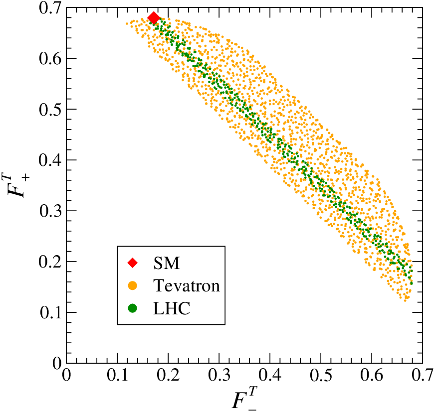
The variation of $F^{T}_{\pm}$ for $Wtb$ couplings inside these regions is shown in Fig. 7. We also mark the value corresponding to the SM prediction. Notice that when anomalous couplings are present $F^{T}_{+}$ takes values smaller than the SM one, in agreement with Fig. 2. This plot demonstrates that, given the present (and expected) constraints on helicity fractions, there is still large room for departures from the SM prediction for $F^{T}_{+}$, $F^{T}_{-}$. Hence, their measurement is necessary and will provide useful constraints on the $Wtb$ vertex. For real anomalous couplings, the normal polarisation fractions are fixed by the sum rule in Eq. (13) once that helicity fractions are measured, and the corresponding plot is not shown.

The $1\sigma$ limits on anomalous couplings for the general case are presented in Fig. 8. On the upper row we show the limits on $V_{L}$ (taken real and positive by definition) and the real parts of $V_{R}$, $g_{L}$ and $g_{R}$. These plots correspond to the ones shown in Fig. 6 but the allowed regions are larger, because with three more free parameters in the fits there is more room for cancellations among different contributions. In the lower row we show the limits on the real and imaginary parts of the anomalous couplings $V_{R}$, $g_{L}$ and $g_{R}$. For the first two, helicity fractions and single top cross sections basically set limits on $|V_{R}|^{2}$ and $|g_{L}|^{2}$, respectively.⁸⁸ 8 This fact does not contradict our previous claim that linear terms in $V_{R}$, $g_{L}$ proportional to the $b$ quark mass are important, because here the limits are rather loose due to the few number of observables included and the possibility of cancellations. Indeed, the important effect of the $b$ quark mass can be clearly appreciated in the results presented in section 9. The limits on $g_{R}$, for a fixed $V_{L}$, have a ring shape in the $(\text{Re}\,g_{R},\text{Im}\,g_{R}$) plane. The resulting regions in Fig. 8 (down, right) are the superposition of several such rings of different centres and radii.

The variation of $F^{T}_{\pm}$, $F^{N}_{\pm}$ for $Wtb$ couplings inside these regions is shown in Fig. 9. We also mark the values corresponding to the SM prediction. For $F^{T}_{\pm}$ the allowed range is very large, practically the same as in the real case. For $F^{N}_{\pm}$, we also observe that there is ample room for departures from the SM equality $F^{N}_{+}=F^{N}_{-}$. Therefore, their determination is quite interesting in order to explore new physics contributing to the $Wtb$ vertex, in particular if the anomalous couplings have complex phases.

The presence of anomalous $Wtb$ couplings influences the angular distribution of the $W$ boson produced in the decay $t\to Wb$, in addition to its polarisation. Indirectly, the angular distribution in the top quark rest frame of the $W$ decay products is affected by both. Then, it is pertinent to ask ourselves about the relation between the measurement of transverse and normal $W$ polarisations and the distributions of top quark decay products.

For the decay $t\to W^{+}b\to\ell^{+}\nu b,q\bar{q}^{\prime}b$, the angular distribution of any decay product $X=\ell^{+},\nu,q,\bar{q}^{\prime},W^{+},b$ (which are called “spin analysers”) in the top quark rest frame is given by

$$\frac{1}{\Gamma}\frac{d\Gamma}{d\!\cos\theta_{X}}=\frac{1}{2}(1+\alpha_{X}\cos\theta_{X})$$

(29)

with $\theta_{X}$ the angle between the three-momentum of $X$ in the $t$ rest frame and the top spin direction. The constants $\alpha_{X}$ are called “spin analysing power” of $X$ and can range between $-1$ and $1$. In the SM $\alpha_{\ell^{+}}=\alpha_{\bar{q}^{\prime}}=1$, $\alpha_{\nu}=\alpha_{q}=-0.32$ and $\alpha_{b}=-\alpha_{W^{+}}=-0.41$ at the tree level [20] ($q$ and $q^{\prime}$ are the up- and down-type quarks, respectively, resulting from the $W$ decay). One-loop corrections slightly modify these values to $\alpha_{\ell^{+}}=0.998$, $\alpha_{\bar{q}^{\prime}}=0.93$, $\alpha_{\nu}=-0.33$, $\alpha_{q}=-0.31$, $\alpha_{b}=-\alpha_{W^{+}}=-0.39$ [48, 49, 50]. We have calculated the spin analysing power constants for the general (complex) $Wtb$ vertex in Eq. (1), keeping $m_{b}$ non-zero and quadratic terms in the couplings, generalising previous results in the literature [51, 52, 38]. The spin analysing power constants can be written as $\alpha_{X}=a_{X}/a_{0}$, with

	$\displaystyle a_{0}$	$\displaystyle=\left[|V_{L}|^{2}+|V_{R}|^{2}\right]\left(1+x_{W}^{2}-2x_{W}^{4}\right)+2\left[|g_{L}|^{2}+|g_{R}|^{2}\right]\left(1-\frac{x_{W}^{2}}{2}-\frac{x_{W}^{4}}{2}\right)$
		$\displaystyle-12x_{W}^{2}x_{b}\,\text{Re}\,\left[V_{L}V_{R}^{*}+g_{L}g_{R}^{*}\right]-6x_{W}\text{Re}\,\left[V_{L}g_{R}^{*}+V_{R}g_{L}^{*}\right]\left(1-x_{W}^{2}\right)$
		$\displaystyle+6x_{W}x_{b}\,\text{Re}\,\left[V_{L}g_{L}^{*}+V_{R}g_{R}^{*}\right]\,,$
	$\displaystyle a_{b}$	$\displaystyle=-2\frac{|\vec{q}\,|}{m_{t}}\left\{\left[|V_{L}|^{2}-|V_{R}|^{2}\right]\left(1-2x_{W}^{2}\right)+2\left[|g_{L}|^{2}-|g_{R}|^{2}\right]\left(1-\frac{x_{W}^{2}}{2}\right)\right.$
		$\displaystyle\left.+2x_{W}\,\text{Re}\,\left[V_{L}g_{R}^{*}-V_{R}g_{L}^{*}\right]+6x_{W}x_{b}\,\text{Re}\,\left[V_{L}g_{L}^{*}-V_{R}g_{R}^{*}\right]\right\}\,,$
	$\displaystyle a_{\ell^{+}}$	$\displaystyle=\left[|V_{L}|^{2}-|V_{R}|^{2}\right]\left(1+x_{W}^{2}-2x_{W}^{4}\right)+2\left[|g_{L}|^{2}-|g_{R}|^{2}\right]\left(1-\frac{x_{W}^{2}}{2}-\frac{x_{W}^{4}}{2}\right)$
		$\displaystyle-12x_{W}^{2}x_{b}\,\text{Re}\,\left[V_{L}V_{R}^{*}+g_{L}g_{R}^{*}\right]-6x_{W}\,\text{Re}\,\left[V_{L}g_{R}^{*}+V_{R}g_{L}^{*}\right]\left(1-x_{W}^{2}\right)$
		$\displaystyle+6x_{W}x_{b}\,\text{Re}\,\left[V_{L}g_{L}^{*}-V_{R}g_{R}^{*}\right]\left(1+x_{W}^{2}\right)+12x_{W}^{2}\left[|V_{R}|^{2}-|g_{R}|^{2}\right]$
		$\displaystyle+6\frac{M_{W}}{|\vec{q}\,|}x_{W}\log\frac{E_{W}+|\vec{q}\,|}{E_{W}-|\vec{q}\,|}\left[|g_{R}|^{2}-x_{W}^{2}|V_{R}|^{2}+2x_{W}x_{b}\,\text{Re}\,V_{R}g_{R}^{*}\right]\,,$
	$\displaystyle a_{\nu}$	$\displaystyle=\left[|V_{L}|^{2}-|V_{R}|^{2}\right]\left(1+x_{W}^{2}-2x_{W}^{4}\right)+2\left[|g_{L}|^{2}-|g_{R}|^{2}\right]\left(1-\frac{x_{W}^{2}}{2}-\frac{x_{W}^{4}}{2}\right)$
		$\displaystyle+12x_{W}^{2}x_{b}\,\text{Re}\,\left[V_{L}V_{R}^{*}+g_{L}g_{R}^{*}\right]+6x_{W}\,\text{Re}\,\left[V_{L}g_{R}^{*}+V_{R}g_{L}^{*}\right]\left(1-x_{W}^{2}\right)$
		$\displaystyle+6x_{W}x_{b}\,\text{Re}\,\left[V_{L}g_{L}^{*}-V_{R}g_{R}^{*}\right]\left(1+x_{W}^{2}\right)-12x_{W}^{2}\left[|V_{L}|^{2}-|g_{L}|^{2}\right]$
		$\displaystyle-6\frac{M_{W}}{|\vec{q}\,|}x_{W}\log\frac{E_{W}+|\vec{q}\,|}{E_{W}-|\vec{q}\,|}\left[|g_{L}|^{2}-x_{W}^{2}|V_{L}|^{2}+2x_{W}x_{b}\,\text{Re}\,V_{L}g_{L}^{*}\right]\,,$		(30)

with $E_{W}^{2}=M_{W}^{2}+|\vec{q}\,|^{2}$. In the above expressions we have omitted for brevity terms of order $x_{b}^{2}$ and higher, which are kept in our numerical code anyway. For the rest of top quark decay products we have $a_{\bar{q}^{\prime}}=a_{\ell^{+}}$, $a_{q}=a_{\nu}$ and $a_{W^{+}}=-a_{b}$. The angular distributions for the decay of a top antiquark are the same, with $\alpha_{\bar{X}}=-\alpha_{X}$ even in the CP-violating case, as obtained by an explicit calculation. We point out that imaginary parts of coupling products do not directly enter these expressions (only through the moduli squared). Although they appear in the matrix element squared involved in the evaluation of $a_{\ell}$ and $a_{\nu}$ they cancel when integrated over the azimuthal angle $\psi_{X}$ of the the spin analyser momentum with respect to the top spin. The dependence of spin analysing powers on the real and imaginary parts of anomalous couplings is shown in Fig. 10. We consider only one anomalous coupling non-zero at a time, and show separately the dependence on the real and imaginary parts.

References

- [1] M. Beneke et al., hep-ph/0003033.
- [2] C. E. Gerber et al. [TeV4LHC-Top and Electroweak Working Group], 0705.3251 [hep-ph].
- [3] W. Bernreuther, J. Phys. G 35, 083001 (2008) [0805.1333 [hep-ph]].
- [4] P. Nath et al., Nucl. Phys. Proc. Suppl. 200-202 (2010) 185 [1001.2693 [hep-ph]].
- [5] C. J. C. Burgess and H. J. Schnitzer, Nucl. Phys. B 228 (1983) 464.
- [6] C. N. Leung, S. T. Love and S. Rao, Z. Phys. C 31 (1986) 433.
- [7] W. Buchmuller and D. Wyler, Nucl. Phys. B 268 (1986) 621.
- [8] J. A. Aguilar-Saavedra, Nucl. Phys. B 812 (2009) 181 [0811.3842 [hep-ph]]; Nucl. Phys. B 821 (2009) 215 [0904.2387 [hep-ph]].
- [9] O. Antipin and G. Valencia, Phys. Rev. D 79 (2009) 013013 [0807.1295 [hep-ph]].
- [10] S. K. Gupta, A. S. Mete and G. Valencia, Phys. Rev. D 80 (2009) 034013 [0905.1074 [hep-ph]].
- [11] S. K. Gupta and G. Valencia, Phys. Rev. D 81 (2010) 034013 [0912.0707 [hep-ph]].
- [12] J. A. Aguilar-Saavedra, Phys. Rev. D 67 (2003) 035003 [Erratum-ibid. D 69 (2004) 099901] [hep-ph/0210112].
- [13] F. del Aguila, M. Perez-Victoria and J. Santiago, Phys. Lett. B 492 (2000) 98 [hep-ph/0007160]; JHEP 0009 (2000) 011 [hep-ph/0007316].
- [14] J. j. Cao, R. J. Oakes, F. Wang and J. M. Yang, Phys. Rev. D 68 (2003) 054019 [hep-ph/0306278].
- [15] X. l. Wang, Q. l. Zhang and Q. p. Qiao, Phys. Rev. D 71 (2005) 014035 [hep-ph/0501145].
- [16] A. Pomarol and J. Serra, Phys. Rev. D 78, 074026 (2008) [0806.3247 [hep-ph]].
- [17] W. Bernreuther, P. Gonzalez and M. Wiebusch, Eur. Phys. J. C 60 (2009) 197 [0812.1643 [hep-ph]].
- [18] G. L. Kane, G. A. Ladinsky and C. P. Yuan, Phys. Rev. D 45 (1992) 124.
- [19] M. Jezabek and J. H. Kuhn, Phys. Lett. B 329 (1994) 317 [hep-ph/9403366].
- [20] M. Jezabek, Nucl. Phys. Proc. Suppl. 37B (1994) 197 [hep-ph/9406411].
- [21] A. Brandenburg and J. P. Ma, Phys. Lett. B 298 (1993) 211.
- [22] W. Bernreuther and A. Brandenburg, Phys. Rev. D 49 (1994) 4481 [hep-ph/9312210].
- [23] J. Bernabeu, G. A. Gonzalez-Sprinberg and J. Vidal, Phys. Lett. B 326 (1994) 168.
- [24] R. Alemany, N. Rius, J. Bernabeu, J. J. Gomez-Cadenas and A. Pich, Nucl. Phys. B 379 (1992) 3.
- [25] J. Bernabeu, G. A. Gonzalez-Sprinberg and J. Vidal, Nucl. Phys. B 763 (2007) 283 [hep-ph/0610135].
- [26] J. Bernabeu, G. A. Gonzalez-Sprinberg, J. Papavassiliou and J. Vidal, Nucl. Phys. B 790, 160 (2008) [0707.2496 [hep-ph]].
- [27] G. Mahlon and S. J. Parke, Phys. Lett. B 476 (2000) 323 [hep-ph/9912458].
- [28] D. Dicus, A. Stange and S. Willenbrock, Phys. Lett. B 333, 126 (1994) [hep-ph/9404359].
- [29] W. Bernreuther, M. Flesch and P. Haberl, Phys. Rev. D 58, 114031 (1998) [hep-ph/9709284].
- [30] D. Choudhury, R. M. Godbole, R. K. Singh and K. Wagh, Phys. Lett. B 657 (2007) 69 [0705.1499 [hep-ph]].
- [31] T. M. P. Tait and C. P. Yuan, Phys. Rev. D 63 (2001) 014018 [hep-ph/0007298].
- [32] Q. H. Cao, J. Wudka and C. P. Yuan, Phys. Lett. B 658 (2007) 50 [0704.2809 [hep-ph]].
- [33] J. A. Aguilar-Saavedra, Nucl. Phys. B 837 (2010) 122 [1003.3173 [hep-ph]].
- [34] R. H. Dalitz and G. R. Goldstein, Phys. Rev. D 45, 1531 (1992).
- [35] J. A. M. Vermaseren, math-ph/0010025.
- [36] C. R. Chen, F. Larios and C. P. Yuan, Phys. Lett. B 631 (2005) 126 [AIP Conf. Proc. 792 (2005) 591] [hep-ph/0503040].
- [37] D. Espriu and J. Manzano, Phys. Rev. D 65 (2002) 073005 [hep-ph/0107112]; Phys. Rev. D 66 (2002) 114009 [hep-ph/0209030].
- [38] J. A. Aguilar-Saavedra, J. Carvalho, N. Castro, A. Onofre and F. Veloso, Eur. Phys. J. C 50 (2007) 519 [hep-ph/0605190].
- [39] G. Aad et al. [ATLAS Collaboration], 0901.0512 [hep-ex].
- [40] G. L. Bayatian et al. [CMS Collaboration], J. Phys. G 34 (2007) 995.
- [41] A. Czarnecki, J. G. Korner and J. H. Piclum, 1005.2625 [hep-ph].
- [42] J. A. Aguilar-Saavedra, Nucl. Phys. B 804 (2008) 160 [0803.3810 [hep-ph]].
- [43] B. Lampe, Nucl. Phys. B 454 (1995) 506.
- [44] F. del Aguila and J. A. Aguilar-Saavedra, Phys. Rev. D 67 (2003) 014009 [hep-ph/0208171].
- [45] J. A. Aguilar-Saavedra, J. Carvalho, N. F. Castro, A. Onofre and F. Veloso, Eur. Phys. J. C 53 (2008) 689 [0705.3041 [hep-ph]].
- [46] T. Aaltonen et al. [CDF Collaboration], 1003.0224 [hep-ex].
- [47] T. Aaltonen et al. [CDF Collaboration], Phys. Rev. Lett. 103 (2009) 092002 [0903.0885 [hep-ex]]
- [48] A. Czarnecki, M. Jezabek and J. H. Kuhn, Phys. Lett. B 346 (1995) 335 [hep-ph/9411282].
- [49] A. Brandenburg, Z. G. Si and P. Uwer, Phys. Lett. B 539 (2002) 235 [hep-ph/0205023].
- [50] W. Bernreuther, A. Brandenburg, Z. G. Si and P. Uwer, Nucl. Phys. B 690, 81 (2004) [hep-ph/0403035].
- [51] B. Grzadkowski and Z. Hioki, Phys. Lett. B 476 (2000) 87 [hep-ph/9911505]; Phys. Lett. B 557 (2003) 55 [hep-ph/0208079].
- [52] R. M. Godbole, S. D. Rindani and R. K. Singh, JHEP 0612, 021 (2006) [hep-ph/0605100].
- [53] J. A. Aguilar-Saavedra, J. Carvalho, N. Castro, M. C. N. Fiolhais, A. Onofre and F. Veloso, Nuovo Cim. 123B (2008) 1323.
- [54] G. Mahlon and S. J. Parke, Phys. Rev. D 53 (1996) 4886 [hep-ph/9512264].
- [55] T. Stelzer and S. Willenbrock, Phys. Lett. B 374, 169 (1996) [hep-ph/9512292].
- [56] W. Bernreuther and Z. G. Si, 1003.3926 [hep-ph].
- [57] F. Hubaut, E. Monnier, P. Pralavorio, K. Smolek and V. Simak, Eur. Phys. J. C 44S2 (2005) 13 [hep-ex/0508061].
- [58] J. A. Aguilar-Saavedra and A. Onofre, 1002.4718 [hep-ph].
- [59] B. Grzadkowski and M. Misiak, Phys. Rev. D 78 (2008) 077501 [0802.1413 [hep-ph]].
- [60] E. Barberio et al. [Heavy Flavor Averaging Group], 0808.1297 [hep-ex].
- [61] F. Larios, M. A. Perez and C. P. Yuan, Phys. Lett. B 457 (1999) 334 [hep-ph/9903394].