Flat-lens focusing of electrons on the surface of a topological insulator

Consider an electron propagating approximately along the $x$-axis (the optical axis) and impinging at $x=0$ onto an electrostatic potential step $\delta U$ produced by a gate electrode (see Fig. 1). For simplicity, we assume that the optical axis is parallel to an axis of crystallographic symmetry, such that the equi-energy contours are $\pm k_{y}$ symmetric. (For the more general case, see App. A.) At constant Fermi energy, the kinetic energy changes from $E_{i}$ in the incident (left) region to $E_{t}=E_{i}+\delta U$ in the transmitted (right) region. The equi-energy contour at the left is given locally by $\delta k_{{i},x}=-\frac{1}{2}c_{i}k_{{i},y}^{2}$, for a two-dimensional wave vector ${\bm{k}}_{i}=(k_{{i},0}+\delta k_{{i},x},k_{{i},y})$ approximately along the optical axis, and similarly $\delta k_{{t},x}=-\frac{1}{2}c_{t}k_{{t},y}^{2}$ at the right. The coefficients $c_{i}$ and $c_{t}$ are the curvatures of the Fermi surface for normal incidence, at the two sides of the potential step.

The velocity ${\bm{v}}=\hbar^{-1}\partial E/\partial{\bm{k}}$ is normal to the equi-energy contours, so that the velocities ${\bm{v}}_{i}$ and ${\bm{v}}_{t}$ in the left and right regions make, respectively, an angle $\theta_{i}=c_{i}k_{{i},y}$ and $\theta_{t}=c_{t}k_{{t},y}$ with the $x$-axis. Conservation of transverse momentum ($k_{{i},y}=k_{{t},y}$) leads to the linearized Snell’s law

The inverse curvature plays the role of the refractive index in optics. Negative refraction (meaning $\theta_{i}\theta_{t}<0$) takes place when $c_{i}$ and $c_{t}$ have opposite signs, as illustrated in Fig. 1.

As we will see in the next section, to calculate the image of a point source we will need to include the first nonlinear correction to Eq. (1). In optics, where one has a circular equi-energy contour, Snell’s law $c_{i}\sin\theta_{t}=c_{t}\sin\theta_{i}$ implies the series expansion

with $n_{1}=c_{t}/c_{i}$ and $n_{3}=\frac{1}{6}n_{1}(n_{1}^{2}-1)$. More generally, we can write

where $\Delta$ quantifies the deviation from the optical Snell’s law.[31]

The parameter $\Delta$ vanishes for a circular Fermi surface as in graphene,[12, 29, 30] but is nonzero for the warped Fermi surfaces of topological insulators. In order to relate $\Delta$ to the Fermi surface, we parameterize the equi-energy contour using polar coordinates by ${\bm{k}}=\kappa(\phi)(\cos\phi,\sin\phi)$, where $\phi$ is the angle between the wave vector ${\bm{k}}$ and the $x$-axis and $\kappa=|\bm{k}|$. A subscript $i$ or $t$ distinguishes the parameters at the two sides of the potential step.

The noncircular Snell’s law is expressed by the three equations

where $\kappa^{\prime}=d\kappa/d\phi$. The first equation expresses the continuity of the $y$-component of the wave vector at the interface $x=0$, while the second and third equations relate the angles $\theta$ and $\phi$ of velocity and wave vector (using the fact that ${\bm{v}}$ is perpendicular to the equi-energy contour). The circular Snell’s law $\kappa_{t}\sin\theta_{t}=\kappa_{i}\sin\theta_{i}$ is recovered for $\kappa^{\prime}=0$, when $\theta=\phi$.

Near $\phi=0$, the equi-energy contour can be parameterized in terms of the curvature $c$ and conic constant $\mathcal{K}$,

with $\delta k_{x}=k_{x}-\kappa(0)$. The noncircular Snell’s law then expands to Eqs. (2)–(3) with

We apply these general considerations to the topological insulator Bi₂Te₃. On the $[111]$ surface and close to the center of the Brillouin zone (the $\Gamma$ point) the Hamiltonian can be approximated by[28]

The dispersion relation in the conduction band ($E>0$) is

The $\sigma_{i}$’s are Pauli matrices acting on the electron spin and $\phi$ denotes the angle of the wave vector ${\bm{k}}$ with respect to the $\Gamma$K direction in the Brillouin zone (oriented along the $x$-axis). The parameters $v\approx 4\cdot 10^{5}\,{\rm m/s}$ and $\lambda\approx 1\,$nm were estimated by fitting to data from angularly resolved spectroscopy.[22, 21] (Additional terms quadratic in momentum can be included in the fit, but these do not qualitatively change the dispersion.)

The curvature $c(E)$ of the equi-energy contour in the $\Gamma$K direction is given by

with $\varkappa^{2}=\xi_{+}^{1/3}-\xi_{-}^{1/3}$ defined in terms of

The quantity $\varkappa/\lambda=\kappa(0)$ equals $|\bm{k}|$ at $\phi=0$.

The energy dependence of the curvature is plotted in Fig. 2. As discovered by Fu,[28] the curvature changes sign when $\varkappa_{c}^{4}=1/6$, which corresponds to an energy $E_{c}=6^{-3/4}\sqrt{7}\,\hbar v/\lambda\approx 0.2\,$eV and a wave vector $k_{c}=\varkappa_{c}/\lambda\approx 0.6\,{\rm nm}^{-1}$. At the same point the conic constant

diverges and thereby changes sign, cf. Fig. 3.

Because of the negative refraction, diverging trajectories become converging at the potential step and then cross at a focal point (see Fig. 4). If a point source is placed at $(-a,0)$, a distance $a$ from the interface at $x=0$, then the trajectory for an electron incident at an angle $\theta_{i}$ and transmitted at an angle $\theta_{t}$ is parameterized by

On the optical axis $y,\theta_{i},\theta_{t}\rightarrow 0$ we obtain the focal point $(a_{F},0)$, with

proportional to the ratio of the two curvatures. As in the optical Veselago lens,[32, 33] the focal point is displaced from the optical axis as we increase the angle of incidence, so that the point $(a_{F},0)$ is the cusp on a curve of focal points. This caustic curve (called an astroid[34]) is visible in Fig. 4 as the envelope of the refracted trajectories.

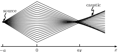
The caustic curve near $(a_{F},0)$ is obtained from Eq. (14) and the nonlinear Snell’s law (2) by demanding that $\partial y/\partial\theta_{i}=0$. We find

with the opening rate of the cusp governed by the parameter

For $\Delta=0$, so for a circular Fermi surface, this agrees with Refs. 12, 33. Depending on the sign of $\alpha$, the cusp points away from the potential step (for $\alpha>0$) or towards the potential step (for $\alpha<0$). For $\alpha=0$ higher than third-order terms in the expansion (2) have to be included in order to obtain the caustic curve.

The diffraction pattern near a cusp caustic has a universal functional form (Pearcey integral),[35, 36] but the parameters governing that function are modified for noncircular equi-energy contours. We calculate the wave function $\Psi$ at a point $\bm{r}=(x,y)$ near the cusp by summing over partial waves $\Psi_{y_{0}}$ from points $\bm{r}_{0}=(0,y_{0})$ along the potential step [excited by a point source at $\bm{r}_{\rm source}=(-a,0)$]. In the far-field approximation, for $a$ and $a_{F}$ large compared to the wave length, the partial waves have the simple form

The amplitude $A_{y_{0}}$ and spinor components $u_{y_{0}},v_{y_{0}}$ vary slowly as $y_{0}$ is varied on the scale of the wave length, so we fix their values at $A_{0},u_{0},v_{0}$ and retain only the $y_{0}$ dependence of the phase $\Phi_{y_{0}}$.

In the optical case, the wave vectors $\bm{k}_{i}$ and $\bm{k}_{t}$ at the two sides of the interface point in the direction of the velocity and hence are parallel to the rays $\bm{r}_{0}-\bm{r}_{\text{source}}$ and $\bm{r}-\bm{r}_{0}$. For a noncircular Fermi surface this is no longer true and we have to take into account the difference between the angles $\phi_{i}$, $\phi_{t}$ and $\theta_{i}={\rm arctan}\,(y_{0}/a)$ and $\theta_{t}={\rm arctan}\,[(y-y_{0})/x]$ which the wave vectors and the rays make with the $x$-axis. The relation between $\phi$ and $\theta$ is expressed by Eqs. (5) and (6), in terms of the radial parameter $\kappa(\phi)=|\bm{k}|$ of the equi-energy contour.

We expand $\Phi_{y_{0}}$ in a power series in $y_{0}$. Near the cusp caustic (16), $y/a={\cal O}(y_{0}/a)^{3}$ while $x/a_{F}-1={\cal O}(y_{0}/a_{F})^{2}$. To fourth order in $y_{0}$ we find

with $\alpha$ given by Eq. (17). One readily checks that the stationary phase equations $\partial\Phi_{y_{0}}/\partial y_{0}=0=\partial^{2}\Phi_{y_{0}}/\partial y_{0}^{2}$ give the caustic curve (16). (These equations correspond to the geometric optics limit $c_{t}\to 0$ of vanishing wavelength.)

The current density $j(\mathbf{r})$ follows upon integration over $y_{0}$,

with $j_{0}$ a constant proportional to the product of the injection rate at the source and the transmission probability $T$ through the potential step. By rescaling the integration variable $y_{0}\to ay^{\prime}_{0}$, we see that the current density (21) as a function of $x/a_{F}$ and $y/a$ depends only on the two parameters $\alpha$ and $a/c_{i}$. Figure 5 is a plot of this current density, showing the characteristic interference pattern of a cusp caustic.

The flat lens in Fig. 6 is formed by the potential profile $U(x)=\delta U$ for $0<x<L$, $U(x)=0$ otherwise. We denote the Fermi surface curvatures (of opposite sign) inside the lens ($0<x<L$) by $c_{\rm lens}$ and outside ($x<0$, $x>L$) by $c_{0}$. Negative refraction at the two potential steps at $x=0$ and $x=L$ focuses a source at $x=-a$ on the optical axis ($y=0$) first onto the point $a_{1}=-(c_{0}/c_{\rm lens})a$ inside the lens and then onto the point

outside the lens (provided it is sufficiently thick, $|c_{\rm lens}L|>|c_{0}a|$).

The classical trajectories are now parameterized by

The relation between $\theta_{t}$ and $\theta_{i}$ is still given by Eq. (2), with

The cusp caustic near $(a_{F},0)$ has the form

as in Eq. (16) but with a different parameter

Notice that $\alpha$ and $\beta$ have the opposite sign (because of the factor $c_{\rm lens}/c_{0}<0$), so that the cusps inside and outside the lens point in opposite directions (as visible in Fig. 6).

The flat-lens diffraction pattern near the caustic is given by the same Pearcey integral (20)–(21) as for a single interface, but with different coefficients,

Thus, the interference pattern that can be observed near $a_{F}$ looks similar to Fig. 5.

The Veselago lens at a p-n junction in graphene[12] uses interband scattering to achieve negative refraction. In contrast, the mechanism considered here is intraband, operating entirely within the conduction band. The p-n junction has one special feature which our setup lacks, which is the possibility to use electron-hole symmetry to collapse the caustic curve onto a single focal point (when $c_{t}=-c_{i}$). In our setup the Fermi surfaces at the two sides of the potential step are not related by any symmetry relation, so in general the two Fermi surface curvatures $c_{t}$ and $c_{i}$ will be different in magnitude.

The main advantage of an intraband over an interband mechanism for negative refraction is that the transmission probability $T$ can be much higher. Typically, the width $d$ of the potential step will be large compared to the Fermi wave length $\lambda_{F}=2\pi/k_{F}$. Intraband transmission is then realized with unit probability, up to exponentially small backscattering corrections: $T=1-{\cal O}(e^{-k_{F}d})$. Interband transmission, in contrast, has $T\simeq\exp(-k_{F}d\sin^{2}\theta_{i})$, so it is exponentially suppressed for angles further than $\sqrt{\lambda_{F}/d}$ from normal incidence.[14]

Realization of the intraband flat lens proposed here, requires firstly a topological insulator with sufficiently long mean free paths to ensure ballistic motion of the electrons from source to focus. Sufficiently pure single crystals should make this possible.

Secondly, and more specifically, the curvature of the Fermi surface should be tunable from positive to negative values by a gate voltage. From spectroscopic data[22] for Sn-doped Bi₂Te₃ we would estimate that a potential step $\delta U\simeq-0.1\,$eV would produce a positive curvature inside a narrow strip and a negative curvature outside (as in Fig. 6). The strip itself would also allow for bulk conduction, because in Bi₂Te₃ a positively curved Dirac cone of surface states overlaps with bulk states. Since the regions outside the lens have only surface conduction, we do not expect the bulk states inside the lens to spoil the focusing.

A point source can be created, for example, using the “needle-anvil” technique developed for point contact spectroscopy,[37] or alternatively using a scanning tunneling microscope (STM). For the spatially resolved detection of the current density distribution an STM tip is most convenient. Such a setup would provide a sensitive probe of the nonspherical Fermi surface of a topological insulator, in a similar way as has recently been proposed for metals.[38]

References

- [1] J. Spector, J. S. Weiner, H. L. Störmer, K. W. Baldwin, L. N. Pfeiffer, and K. W. West, Surf. Sci. 263, 240 (1992).
- [2] H. van Houten and C. W. J. Beenakker, in Confined Electrons and Photons: New Physics and Applications, ed. by E. Burstein and C. Weisbuch, NATO ASI Series B 340, 269 (Plenum, New York, 1995).
- [3] B. J. LeRoy, J. Phys. Cond. Matt. 15, R1835 (2003).
- [4] M. A. Topinka, R. M. Westervelt, and E. J. Heller, Phys. Today 56 (12), 47 (2003).
- [5] J. Spector, H. L. Störmer, K. W. Baldwin, L. N. Pfeiffer, and K. W. West, Appl. Phys. Lett. 56, 967 (1990).
- [6] U. Sivan, M. Heiblum, C. P. Umbach, and H. Shtrikman, Phys. Rev. B 41, 7937 (1990).
- [7] V. G. Veselago, Sov. Phys. Usp. 10, 509 (1960).
- [8] J. B. Pendry and D. R. Smith, Phys. Today 57 (6), 37 (2004).
- [9] M. Notomi, Phys. Rev. B 62, 10696 (2000).
- [10] P. V. Parimi, W. T. Lu, P. Vodo, and S. Sridhar, Nature 426, 404 (2003).
- [11] E. Cubukcu, K. Aydin, E. Ozbay, S. Foteinopoulou, and C. M. Soukoulis, Nature 423, 604 (2003).
- [12] V. V. Cheianov, V. Fal’ko, and B. L. Al’tshuler, Science 315, 1252 (2007).
- [13] M. I. Katsnelson, K. S. Novoselov, and A. K. Geim, Nature Phys. 2, 620 (2006).
- [14] V. V. Cheianov and V. I. Fal’ko, Phys. Rev. B 74, 041403 (2006).
- [15] X.-L. Qi and S.-C. Zhang, Phys. Today 63 (1), 33 (2010).
- [16] M. Z. Hasan and C. L. Kane, arXiv:1002.3895.
- [17] P. Roushan, J. Seo, C. V. Parker, Y. S. Hor, D. Hsieh, D. Qian, A. Richardella, M. Z. Hasan, R. J. Cava, and A. Yazdani, Nature 460, 1106 (2009).
- [18] T. Zhang, P. Cheng, X. Chen, J.-F. Jia, X. Ma, K. He, L. Wang, H. Zhang, X. Dai, Z. Fang, X. Xie, and Q.-K. Xue, Phys. Rev. Lett. 103, 266803 (2009).
- [19] H. Zhang, C.-X. Liu, X.-L. Qi, X. Dai, Z. Fang, and S.-C. Zhang, Nature Phys. 5, 438 (2009).
- [20] Y. Xia, D. Qian, D. Hsieh, L. Wray, A. Pal, H. Lin, A. Bansil, D. Grauer, Y. S. Hor, R. J. Cava, and M. Z. Hasan, Nature Phys. 5, 398 (2009).
- [21] D. Hsieh, Y. Xia, D. Qian, L. Wray, J. H. Dil, F. Meier, J. Osterwalder, L. Patthey, J. G. Checkelsky, N. P. Ong, A. V. Fedorov, H. Lin, A. Bansil, D. Grauer, Y. S. Hor, R. J. Cava, and M. Z. Hasan, Nature 460, 1101 (2009).
- [22] Y. L. Chen, J. G. Analytis, J.-H. Chu, Z. K. Liu, S.-K. Mo, X. L. Qi, H. J. Zhang, D. H. Lu, X. Dai, Z. Fang, S. C. Zhang, I. R. Fisher, Z. Hussain, and Z.-X. Shen, Science 325, 178 (2009).
- [23] M. Z. Hasan, H. Lin, and A. Bansil, Physics 2, 108 (2009).
- [24] Z. Alpichshev, J. G. Analytis, J.-H. Chu, I. R. Fisher, Y. L. Chen, Z. X. Shen, A. Fang, and A. Kapitulnik, Phys. Rev. Lett. 104, 016401 (2010).
- [25] X. Zhou, C. Fang, W.-F. Tsai, and J. Hu, Phys. Rev. B 80, 245317 (2009).
- [26] W.-C. Lee, C. Wu, D. P. Arovas, and S.-C. Zhang, Phys. Rev. B 80, 245439 (2009).
- [27] Q.-H. Wang, D. Wang, and F.-C. Zhang, Phys. Rev. B 81, 035104 (2010).
- [28] L. Fu, Phys. Rev. Lett. 103, 266801 (2009).
- [29] J. Cserti, A. Pályi, and Cs. Péterfalvi, Phys. Rev. Lett. 99, 246801 (2007).
- [30] Cs. Péterfalvi, A. Pályi, and J. Cserti, Phys. Rev. B 80, 075416 (2009).
- [31] We assume that the potential step is perpendicular to the K direction in Fig. 2, so that only odd powers of appear in the expansion (2). This assumption is relaxed in App. A.
- [32] A. P. Anyutin, J. Comm. Techn. Electr. 53, 387 (2008).
- [33] M. L. Shendeleva, J. Microsc. 229, 452 (2008).
- [34] E. H. Lockwood, A Book of Curves (Cambridge University, Cambridge, 1961).
- [35] T. Pearcey, Phil. Mag. 37, 311 (1946).
- [36] M. V. Berry and C. Upstill, Prog. Opt. 18, 257 (1980).
- [37] Yu. G. Naidyuk and I. K. Yanson, Point Contact Spectroscopy (Springer, Berlin, 2005).
- [38] A. Weismann, M. Wenderoth, S. Lounis, P. Zahn, N. Quaas, R. G. Ulbrich, P. H. Dederichs, and S. Blügel, Science 323, 1190 (2009).
- [39] J. F. Nye and J. H. Hannay, J. Mod. Optics 31 115 (1984).