Cosmological Model-independent Gamma-ray Bursts Calibration and its Cosmological Constraint to Dark Energy
Abstract
As so far, the redshift of Gamma-ray bursts (GRBs) can extend to which makes it as a complementary probe of dark energy to supernova Ia (SN Ia). However, the calibration of GRBs is still a big challenge when they are used to constrain cosmological models. Though, the absolute magnitude of GRBs is still unknown, the slopes of GRBs correlations can be used as a useful constraint to dark energy in a completely cosmological model independent way. In this paper, we follow Wang’s model-independent distance measurement method and calculate their values by using GRBs events via the so-called Amati relation. Then, we use the obtained model-independent distances to constrain CDM model as an example.
1 Introduction
Since the discovery of an accelerated expansion of our Universe through the observations of supernova Ia (SN Ia) [1, 2], many cosmic observations have been used to explore the nature of dark energy which has negative pressure and pushes the Universe into an accelerated phase. Particularly, the redshift of Gamma-ray burst (GRBs) can extend to higher redshift . This merit makes it as a complementary cosmic probe to SN Ia. However, a big challenge, the so-called circular problem, has to be overcome when one calibrates the GRBs to obtain the distances at different redshifts. In [3], Schaefer et. al. have derived the distance modulus in CDM model by using five GRBs correlations. The so-called circular problem would be committed when one uses the resulted distance redshift relation to constrain any other cosmological models beyond CDM. To overcome this circular problem, Li, et. al [4] put the GRBs correlation and cosmological model constraint together. Via the Markov Chain Monte Carlo (MCMC) method, they fixed the calibration parameters and constrained the model parameter space simultaneously. However, it looks like using a ’ruler’ having no marks to measure the length of an object. And after the measurement, the length and scale of ruler are given together. So the lack of calibration makes the GRBs lose the power to constrain cosmological models. Cosmography method was considered in [5] by parameterizing the luminosity distance in terms of deceleration , jerk and snap parameters. In this way, the cosmological model dependent problem was removed. Liang et. al. [6] calibrated GRBs by using low redshift SN Ia and obtained a tight constrain to the cosmological model parameter space. This method was reconsidered by Wei [7, 8]. By analyzing the calibration process carefully, one can find the potential drawback. The calibrated GRBs correlation makes GRBs have the same luminosity distance-redshifts relation as SN Ia at lower redshifts. In this way, the relation is extended to higher redshifts. Equivalently, one just extends the luminosity distance-redshifts relation of SN Ia to higher redshifts. So, it makes the obtained luminosity distance-redshifts relation strongly depends on that of SN Ia. The worst thing is that it makes the data points of GRBs useless, because one has known the luminosity distance-redshifts relation at high redshifts from SN Ia, though no SN Ia is found at the high redshift regions of GRBs. Alternatively, Wang presented a model-independent distance measurement from GRBs calibrated internally [18]. The main point of Wang’s method is that the statistical errors of correlation parameters , and systematic error obtained in CDM models are used, but are not the correlation parameters and themselves, for the definitions of , please see Eq. (2). The viability of this implement comes from the observations that the errors of correlation parameters are almost the same for different values of for CDM model, though the values of and are really different. Then, in terms of a set of model-independent distance measurements, the cosmic constraint from GRBs is set up via cubic spline interpolation from cosmological model independent distance ratio . The merits of this method are follows: (i) the constraint from GRBs is in a cosmological model independent way. It alleviates the circular problem. So, it can be used to constrain any other cosmological models. (ii) It is not calibrated by any other external data sets. It does not suffer any consistent problem when it is combined with other data sets as cosmic constraints. (iii) The cosmological model independent calibration is done firstly. It means that the ’ruler’ has been marked. (iv) Though the absolute magnitude of GRBs is unkown, the slopes of GRBs correlations can be used as cosmological constraints.
Recently, Wei [8] used GRBs data points via Amati relation [11, 12, 13] calibrated by SN Ia to constrain cosmological model. Based on the points mentioned above, to alleviate the data sets dependence and circular problem, we shall present our calculation results based on Wang’s method via Amati correlation. In fact, we find a new which only depends on the slopes of GRBs correlation and make the absolute magnitude of GRBs irrelevant. For the details, please see section 2. As results, a set of model-independent distance measurements are obtained on the basis of Amati relation that can be used to constrain cosmological models.
However we have to stress that the Amati relation has been criticized for many reasons in the literatures. Li demonstrated an ambiguity in determining the redshifts of GRBs [14]. Of course, this ambiguity can be overcome when the redshift is well determined. The major criticism came from Nakar and Prian [15] who developed a test for the Amati relation even in the case where the redshifts of GRBs were unknown. The test was also generalized by Band and Preece [16]. They concluded that the Amati relation suffered the problem of selection bias. Recently, the authors of [17] have also concluded that the Amati relation is an artifact of selection effects with the burst population and the detector. They also point out that the Amati relation is failed whether or not the bursts have measured spectroscopic redshifts. If this is true for Amati relation, the results obtained based on Amati relation would be unreliable. But it is still in debating. So, before the dust settles down, we still assume that Amati relation is reliable in this paper.
This paper is structured as follows. In section 2, the values of cosmological parameter dependance in CDM model are presented as shown in [18]. The errors of correlation parameters , and systematic error are also calculated via Amati relation with GRBs data points. The bins model-independent distance measurements will also be found in this section. In section III, we use the resulted data points to constrain CDM model as an example. A summary and discussion are put in section IV.
2 Calibration of GRBs and Model-independent Distance Measurement
Following the work of [3], we consider the well-known Amati correlation [9, 11, 12, 13] in GRBs, where is the cosmological rest-frame spectral peak energy, and is the isotropic energy
| (1) |
in which and are the luminosity distance and the bolometric fluence of the GRBs respectively. Following [3], we rewrite the Amati relation in the form of
| (2) |
One fitts the Amati relation through the minimization of which is given by [3]
| (3) |
where
| (4) | |||||
| (5) |
where is defined as [18]
| (6) |
and the errors are calculated by using the error propagation law [10]:
| (7) | |||||
| (8) |
By calculating the value of , we find it is large and dominated by the systematic errors, and on the contrast the statistical errors on and are small. Following [3], the systematic error can be derived by required (the degrees of freedom). At last, the total error is obtained. It would be noticed that in our case, the best fit value of will be less than that in the definition of luminosity distance [18]. For this definition, the value of is absorbed into the calibration of GRBs because of the lack of fixing the absolute magnitude of GRBs. Then, in our treatment the results will be free.
As shown in [18], the calibration of GRBs is cosmological model dependent, because the values of and are obtained on the basis of CDM model. So the calibrated result can not be used to constrain any other cosmological models. This the so-called well-known model dependent problem or circular problem. In Tab. 1, the cosmological parameter dependence are shown. With a careful observation, one can find that the errors bars of , and system are almost the same which do not depend on the cosmological parameters. In this paper as suggested by Wang [18], we shall only use the systematic error and the errors of and in the case of for CDM model as the standard values. That is to say the values of , and will be used in the following sections not the values of and derived from CDM model.
To constrain a cosmological model, one uses a set of model-independent distance measurements :
| (13) |
where is the comoving distance at redshift , is the lowest GRBs redshift11 1 was used in [18]. In this work, the lowest redshift of GRBs is . Here, the definition of is different from Wang’s definition [18] where . In our definition, the distance measurement and is completely free. It can be seen from the facts that the definition of is where is the Hubble parameter. In terms of our definition, can be rewritten as
| (14) |
We divide the redshifts of GRBs into bins, i.e. , and assume the corresponding values of which do not depend on any cosmological models. Then the values of at arbitrary redshift can be obtained by cubic spline interpolation from . So, the values of and , etc at redshift can be found easily. Given each set of , we calibrate the GRBs and calculate the likelihood simultaneously via Eq. (9) by using Markov Chain Monte Carlo (MCMC) method [19]. The MCMC is a global fitting method which is used to determine the cosmological parameters. In adopting the MCMC approach, we generate using Monte Carlo method a chain of sample points distributed in the parameter space according to the posterior probability, using the Metropolis-Hastings algorithm with uniform prior probability distribution. In the parameter space formed by the constraint cosmological parameters, a random set of initial values of the model parameters is chosen to calculate the or the likelihood. Whether the set of parameters can be accepted as an effective Markov chain or not is determined by the Metropolis-Hastings algorithm. The accepted set not only forms a Markov chain, but also provides a starting point for the next process. We then repeat this process until the established convergence accuracy can be satisfied. The convergence is tested by checking the so-called worst e-values [the variance(mean)/mean(variance) of 1/2 chains] [19]. As results, we obtain a set of distances which are independent on any assumption of cosmological parameters. It comes from the observations that, in the process of calibration, the statistical and systematic errors of , and are only used. We do not use any values of and calibrated in CDM model. The important thing is that the statistical and systematic errors , and are almost model parameter independent. Thanks to this feature, this method is model-independent. Here, in the MCMC analysis, we take , and as free parameters. So, the degree of freedoms is . Once these values of are obtained, a cosmological model can be constrained by GRBs via the
| (15) | |||||
| (16) |
where is defined by Eq. (13) and is the covariance matrix. In this way, the constraints from larger observational GRBs data points are projected into relative smaller number of points. Of course, this method can be generalized to discuss other problems.
Now, we present some discussion about the treatment of . Here, we do not calculate the value of at the redshift via its definition (13) according to any cosmological model. Because, if we calculate the value for any cosmological model, a model or cosmological parameter dependence will be introduced again. The values of are fixed by the calibration relation (2), i.e. via the relation
| (17) |
In fact, once this relation is used, one can recast Eq. (9) into the following form
| (18) |
where is defined as
| (19) |
and , the is the total errors of data sets
| (20) |
One can see that the parameter is removed from this new form of . In other words, the information about the slope of GRBs correlation is used alone. So the absolute magnitude of GRBs is irrelevant in this method. Of cause, the can be fixed by consulting a special cosmological model or other data sets. But in that way, the circular problem and data sets relevance problem will come back. Equivalently, the absolute magnitude of GRBs was fixed in a special cosmological model. So, for every possible values of in every running of MCMC, the is calculated. Here, we must keep in mind that the values of parameter are not taken from Tab. 1. It is treated as a free parameter. So, this method is completely cosmological parameter in-dependent and self consistent.
We divide the redshifts into bins and run the MCMC codes which is based on the publicly available CosmoMC package [19]]. The chains have worst e-value which is much smaller than . The resulted model-independent distances and covariance matrix from GRBs are shown in Tab. 2
and Eq. (27). As already mentioned above, is adopted in this work. The correlation matrix is given by
and the corresponding covariance matrix is given by
| (27) |
where
| (28) | |||
| (29) |
here the and are the errors listed in Tab. 2. The marginalized values and the corresponding upper and lower bounds are used when GRBs is used as a cosmological constraint. The distributions of model parameters are shown in Fig.1.

The distance measurements from GRBs via Amati correlation with error bars are shown in Fig. 2, where the solid lines correspond to CDM model with different values of from up to bottom respectively.
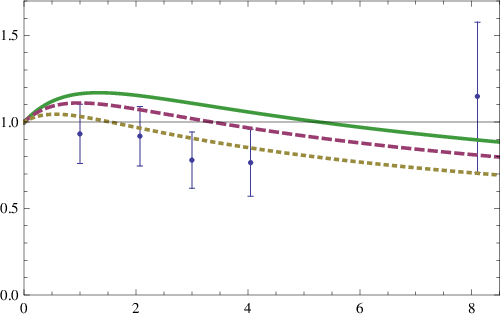
The data points shown in Tab. 2 and Fig. 2 are totally cosmological model independent, so one can use them to constrain any other cosmological models. In the next section, as an example, these obtained data points will be used to constrain CDM model. From Fig. 2, one can find that GRBs favors large values of for CDM model. This point can be confirmed in the next section. And the concordance model () is almost at the boundary of regions of data points. So the null hypothesis that Amati relation is based on cosmology can be rejected slightly greater than as shown in Fig. 2.
3 Cosmological Constraint to Dark Energy
In our calculations, we have taken the total likelihood function to be the products of the separate likelihoods of SN, BAO, CMB and GRBs. Then we get
| (30) |
where the separate likelihoods of SN, BAO, CMB are shown in the Appendix A. The is the form of Eq. (15). In this work, we only consider the CDM model as a simple example. Its generalization to constrain other cosmological models is straight forward. In the case, when SN Ia and GRBs are combined as cosmic constraint, we have and the best fit values of model parameter . If the SN Ia is used alone, one has and . The corresponding contour plot is shown in Fig. 3.

When combing the cosmic observations considered in this work together, we have the resulted and . Also, the best fit values of and when GRBs is not used for comparison. The contour plots are shown in Fig. 4.

We can find that when GRBs is used, the relative errors of model parameters is shrunken. Here, we can compare our result with Wei’s one where he used low redshift GRBs to calibrate the Amati relation. So, we add high redshift data points of GRBs to SN Union 2 data sets. After constraint via MCMC, we have and . The corresponding contour plot is shown in Fig. 5. The constrained results show that relative large values of are favored when GRBs data points are employed. This is consistent with the clues shown in Fig. 2.

4 Summary and Discussion
In this paper, by using GRBs data points via Amati relation, we have derived five data points of distance measurements which do not depend on any cosmological models, i.e. in a model-independent way, based on the method firstly advocated by Wang [18]. Then it can be used to constrain any other cosmological models without the so-called circular and data sets consistence problem. We also find out that the concordance model () is almost at the boundary of regions of data points. So, one can reject the null hypothesis that Amati relation is based on cosmology slightly greater than as shown in Fig. 2.
When GRBs (the five data points of distance measurements) is used as a complementary cosmic constraint to CDM model as an example, the errors of model parameters are shrunken. Though the constraint is not much tighter than that calibrated via low redshift SN, the difference is very small. And, the results can be used to constrain other cosmological model beyond CDM. The important thing is that it does not depend on SN Ia data set. The merits of this method has been mentioned in the introduction. Here, we list possible potential drawbacks of this completely model in-dependent method as follows: (i). The constraint is not much tighter than that obtained from calibration by using SN Ia data points. The looser may come from the lack of enough GRBs data points or the number of bins is not larger. (ii). How to design a cosmological model indicator, here it is model independent distance measurement , which is sensitive to distinguish the cosmological models may be the main points of this method. In this way, the lack of having no enough GRBs data points can be avoided in some senses. (iii) Another negative effect comes from the choice of fiducial redshift . Some average values of would be better.
At last we have to alert the readers that our analysis is based on the assumption that Amati relation is reliable. However, in the literatures, the Amati relation has been criticized for many reasons as mentioned in the introduction. If that is true, our analysis would be unreliable.
Acknowledgements.
The author thanks an anonymous referee for invaluable improvement of this paper and Dr. Jirong Mao for useful discussion on Amati relation. This work is supported by the Fundamental Research Funds for the Central Universities (DUT10LK31) and (DUT11LK39) of P.R. China.Appendix A Cosmic Observations: SN, BAO and CMB
A.1 Type Ia Supernovae constraints
Recently, SCP (Supernova Cosmology Project) collaboration released their Union2 dataset which consists of 557 SN Ia [21]. The distance modulus is defined as
| (31) |
where is the Hubble-free luminosity distance , with the Hubble constant, defined through the re-normalized quantity as , and . Additionally, the observed distance moduli of SN Ia at is
| (32) |
where is their absolute magnitudes.
For the SN Ia dataset, the best fit values of the parameters can be determined by a likelihood analysis, based on the calculation of
| (33) | |||||
where is a nuisance parameter which includes the absolute magnitude and the parameter . The nuisance parameter can be marginalized over analytically [22] as
resulting to
| (34) |
with
Relation (33) has a minimum at the nuisance parameter value , which contains information of the values of and . Therefore, one can extract the values of and provided the knowledge of one of them. Finally, note that the expression
which coincides to Eq. (34) up to a constant, is often used in the likelihood analysis [23, 22], and thus in this case the results will not be affected by a flat distribution.
A.2 Baryon Acoustic Oscillation constraints
The Baryon Acoustic Oscillations are detected in the clustering of the combined the 2dF Galaxy Redshift Survey (2dFGRS) and Sloan Digital Sky Survey (SDSS) main galaxy samples, and measure the distance-redshift relation at . Additionally, Baryon Acoustic Oscillations in the clustering of the SDSS luminous red galaxies measure the distance-redshift relation at . The observed scale of the BAO calculated from these samples, as well as from the combined sample, are jointly analyzed using estimates of the correlated errors to constrain the form of the distance measurement [24, 25, 26]
| (35) |
where for , and respectively. The peak positions of the BAO depend on the ratio of to the sound horizon size at the drag epoch (where baryons were released from photons) , which can be obtained by using a fitting formula [27]:
| (36) |
with
| (37) | |||
| (38) |
In this paper, we use the data of extracted from the Sloan Digitial Sky Survey (SDSS) and the Two Degree Field Galaxy Redshift Survey (2dFGRS) [28], which are listed in Table 3, where is the comoving sound horizon size
| (39) | |||||
where is the sound speed of the photonbaryon fluid [29, 30, 31]:
| (40) |
and here for .
Thus, the is given as
| (44) |
where is a column vector formed from the values of theory minus the corresponding observational data, with
and denotes its transpose.
A.3 Cosmic Microwave Background constraints
The CMB shift parameter is provided by [32]
| (48) |
here, the redshift (the decoupling epoch of photons) is obtained using the fitting function [33]
where the functions and read
In additional, the acoustic scale is related to the first distance ratio and is expressed as
| (49) |
| , | |||
|---|---|---|---|
References
- (1) A. G. Riess, et al., Astron. J. 116 1009(1998) [astro-ph/9805201].
- (2) S. Perlmutter, et al., Astrophys. J. 517 565(1999) [astro-ph/9812133].
- (3) B. E. Schaefer, Astrophys. J. 660, 16 (2007) [astro-ph/0612285].
- (4) H. Li, J. Q. Xia, J. Liu, G. B. Zhao, Z. H. Fan, X. Zhang, Astrophys. J. 680, 92(2008).
- (5) S. Capozziello, L. Izzo, Astron. Astrophys, 490, 31( 2008); V. Vitagliano, J. Q. Xia, S. Liberati, M. Viel, JCAP03(2010)005.
- (6) N. Liang, W. K. Xiao, Y. Liu and S. N. Zhang, Astrophys. J. 685, 354 (2008) [arXiv:0802.4262]; N. Liang and S. N. Zhang, AIP Conf. Proc. 1065, 367 (2008) [arXiv:0808.2655]; T. S. Wang and N. Liang, arXiv:0910.5835 [astro-ph.CO]; N. Liang, P. Wu and S. N. Zhang, Phys. Rev. D 81, 083518 (2010) [arXiv:0911.5644]; H. Gao, N. Liang and Z. H. Zhu, arXiv:1003.5755 [astro-ph.CO].
- (7) H. Wei and S. N. Zhang, Eur. Phys. J. C 63, 139 (2009) [arXiv:0808.2240];
- (8) H. Wei, JCAP1008:020(2010), arXiv:1004.4951 [astro-ph.CO].
- (9) L. Amati et al., Astron. Astrophys. 390, 81 (2002) [astro-ph/0205230].
- (10) Herman J. Mosquera Cuesta, Habib Dumet M., Cristina Furlanetto, JCAP0807,004(2008).
- (11) L. Amati et al., Mon. Not. Roy. Astron. Soc. 391, 577 (2008) [arXiv:0805.0377].
- (12) L. Amati, arXiv:1002.2232 [astro-ph.HE]; L. Amati, Mon. Not. Roy. Astron. Soc. 372, 233 (2006) [astro-ph/0601553].
- (13) L. Amati, F. Frontera and C. Guidorzi, arXiv:0907.0384 [astro-ph.HE].
- (14) L.-X. Li, Mon.Not.Roy.Astron.Soc., Lett, 374, L20(2006).
- (15) E. Nakar, T. Piran, Mon.Not.Roy.Astron.Soc., Lett, 360, L73(2005).
- (16) D. L. Band, R.D. Preece, ApJ, 627, 319(2005).
- (17) A. C. Collazzi, B. E. Schaefer, A. Goldstein, R.D. Preece, arXiv:1112.4347[astro-ph.HE].
- (18) Y. Wang, Phys.Rev.D 78,123532(2008).
- (19) http://cosmologist.info/cosmomc/; A. Lewis and S. Bridle, Phys. Rev. D 66, 103511 (2002).
- (20) W. M. Wood-Vasey et al., Astrophys. J. 666 694 (2007) [astro-ph/0701041].
- (21) R. Amanullah et al. [Supernova Cosmology Project Collaboration], arXiv:1004.1711 [astro-ph.CO].
- (22) S. Nesseris and L. Perivolaropoulos, Phys. Rev. D 72 123519 (2005); L. Perivolaropoulos, Phys. Rev. D 71 063503 (2005); E. Di Pietro and J. F. Claeskens, Mon. Not. Roy. Astron. Soc. 341 1299 (2003); A. C. C. Guimaraes, J. V. Cunha and J. A. S. Lima, JCAP 0910 010 (2009).
- (23) E. Garcia-Berro, E. Gaztanaga, J. Isern, O. Benvenuto and L. Althaus, astro-ph/9907440; A. Riazuelo and J. Uzan, Phys. Rev. D 66 023525 (2002); V. Acquaviva and L. Verde, JCAP 0712 001 (2007).
- (24) T. Okumura, T. Matsubara, D. J. Eisenstein, I. Kayo, C. Hikage, A. S. Szalay and D. P. Schneider, Astrophys. J. 676 889 (2008).
- (25) W. J. Percival et al., arXiv:0907.1660 [astro-ph.CO].
- (26) D. J. Eisenstein et al., [SDSS Collabaration], Astrophys. J. 633 560 (2005) [astro-ph/0501171].
- (27) D. J. Eisenstein and W. Hu, Astrophys. J. 496 605 (1998).
- (28) W. J. Percival et al., Mon. Not. R. Astron. Soc. 381 1053 (2007) arXiv:0705.3323 [astro-ph.CO].
- (29) W. Hu and N. Sugiyama, Astrophys. J. 444 489 (1995) [arXiv:astro-ph/9407093].
- (30) W. Hu, M. Fukugita, M. Zaldarriaga and M. Tegmark, Astrophys. J. 549 669 (2001) [arXiv:astro-ph/0006436].
- (31) R. R. Caldwell and M. Doran, Phys. Rev. D 69 103517 (2004).
- (32) J. R. Bond, G. Efstathiou and M. Tegmark, Mon. Not. Roy. Astron. Soc. 291 L33 (1997).
- (33) W. Hu and N. Sugiyama, Astrophys. J. 471 542 (1996).
- (34) E. Komatsu et al. [WMAP Collaboration], arXiv:1001.4538 [astro-ph.CO].