跳到论文正文
W Papers独立论文阅读器 arXiv:1005.5024 论文正文 计算阅读时间 · 0%
引用这篇论文根据当前论文元数据生成,正式投稿前建议核对。


License: arXiv.org perpetual non-exclusive license
arXiv:1005.5024v2 [math.MG] 02 Jun 2010

Stability results for the volume of random simplices Thanks: The research of the first named author was supported by OTKA grants 75016 and 76099.Thanks:  The second named author was supported by OTKA grants 068398 and 75016, and by the EU Marie Curie IEF project GEOSUMSET

Gergely Ambrus Email address, G. Ambrus : ambrus@renyi.hu and Károly J. Böröczky Email address, K. Böröczky : carlos@renyi.hu Address: Rényi Institute of the Hungarian Academy of Sciences, PO Box 127, 1364 Budapest, Hungary
Abstract.

It is known that for a convex body KK in ℝd\mathbb{R}^{d} of volume one, the expected volume of random simplices in KK is minimised if KK is an ellipsoid, and for d=2d=2, maximised if KK is a triangle. Here we provide corresponding stability estimates.

1. Introduction and history

Let KK be a convex body in ℝd\mathbb{R}^{d}. What is the expected value of the volume of a random simplex in KK? Naturally, this question needs to be clarified further. We will work with two (or three) models: in the first, all the vertices of the simplex are chosen uniformly and independently from KK, while in the second, one vertex is at a fixed position – in a special case, this is the centroid of KK. We are interested in other moments as well, and also, we would like the answer to be invariant under affine transformations.

As a general reference for stochastic geometry, we refer to R. Schneider, W. Weil [40], and for convexity, to T. Bonnesen, W. Fenchel [9], P.M. Gruber [29] and R. Schneider [39]. VV or VdV_{d} stands for the dd-dimensional volume (if the dimension is clear, we shall omit dd), the convex hull of the points x1​…,xnx_{1}\dots,x_{n} is denoted by [x1,…,xn][x_{1},\ldots,x_{n}], and γ⁡(K)\gamma(K) is the centroid of KK.

Definition 1.

Let KK be a convex body in ℝd\mathbb{R}^{d}. For any n⩾d+1n\geqslant d+1 and p>0p>0, let

𝔼np​(K)=V​(K)−n−p​∫K…​∫KV​([x1,…,xn])p​d​x1​…​d​xn.\mathbb{E}^{p}_{n}(K)=V(K)^{-n-p}\int_{K}\ldots\int_{K}V([x_{1},\ldots,x_{n}])^{p}\,dx_{1}\ldots dx_{n}.

Further, for a fixed x∈ℝdx\in\mathbb{R}^{d}, let

𝔼xp​(K)=V​(K)−d−p​∫K…​∫KV​([x,x1,…,xd])p​d​x1​…​d​xd.\mathbb{E}^{p}_{x}(K)=V(K)^{-d-p}\int_{K}\ldots\int_{K}V([x,x_{1},\ldots,x_{d}])^{p}\,dx_{1}\ldots dx_{d}.

Specifically, we write 𝔼∗p​(K)\mathbb{E}^{p}_{*}(K) for 𝔼xp​(K)\mathbb{E}^{p}_{x}(K), when x=γ⁡(K)x=\gamma(K).

In particular, for integer pp, 𝔼d+1p​(K)\mathbb{E}^{p}_{d+1}(K) is the expectation of the pp\,th moment of the relative volume of simplices in KK. Clearly, 𝔼np​(K)\mathbb{E}^{p}_{n}(K) and 𝔼∗p​(K)\mathbb{E}^{p}_{*}(K) are invariant under non-singular affine transformations, and 𝔼op​(K)\mathbb{E}^{p}_{o}(K) is invariant under non-singular linear transformations, where oo stands for the origin. We note that for fixed KK and p⩾1p\geqslant 1, 𝔼xp​(K)\mathbb{E}^{p}_{x}(K) is a strictly convex function of xx, therefore it attains its minimum at a unique point. If KK is oo-symmetric, then the minimum is attained at oo, and 𝔼op​(K)=𝔼∗p​(K)\mathbb{E}^{p}_{o}(K)=\mathbb{E}^{p}_{*}(K).

In the rest of the section, we give an overview of the history of the quantities introduced in Definition 1 and their various connections. The main results are presented in Section 2, whose proofs are found in the subsequent parts. Section 6 contains further corollaries.

1.1. Sylvester’s problem. The quantity 𝔼d+1p​(K)\mathbb{E}^{p}_{d+1}(K) arose right at the first steps of random convex geometry. Indeed, (probably) the first question in this topic is due to Sylvester [42]: in 1864 he (vaguely) asked, what is the probability that four randomly chosen points in a planar convex disc are in convex position, that is, none of them is in the convex hull of the other three. Generalising to higher dimensions, if d+2d+2 points are chosen randomly from a convex body K⊂ℝdK\subset\mathbb{R}^{d}, then the sought quantity is exactly 1−(d+2)​𝔼d+11​(K)1-(d+2)\mathbb{E}^{1}_{d+1}(K). It is then natural to ask: for which convex bodies is this probability minimal and maximal? The first steps in this direction were taken by Blaschke ([6] and [8]), who showed that in the plane, the probability in question is maximal for ellipses, and minimal for triangles. The maximisers in higher dimensions are the ellipsoids (cf. Groemer [26]), whereas the minimiser bodies in higher dimensions are still not known. We shall state these results as theorems later. For a thorough historical account of this problem, see Klee [31], and also Bárány [3].

1.2. Minimisers and affine inequalities. Let K⊂ℝdK\subset\mathbb{R}^{d} be a convex body with γ⁡(K)=0\gamma(K)=0. The intersection body I​KIK of KK is defined by its radial function:

ρI​K​(u)=Vd−1​(K∩u⟂).\rho_{IK}(u)=V_{d-1}(K\cap u^{\perp}).

H. Busemann [16] established the formula

(1) Vd​(K)d−1=(d−1)!2​∫Sd−1Vd−1​(K∩u⟂)d​𝔼o1​(K∩u⟂)​𝑑σ​(u),V_{d}(K)^{d-1}=\frac{(d-1)!}{2}\int_{S^{d-1}}V_{d-1}(K\cap u^{\perp})^{d}\,\mathbb{E}^{1}_{o}(K\cap u^{\perp})d\sigma(u),

where σ\sigma is surface area measure on Sd−1S^{d-1}. In the same paper, he proved the Busemann random simplex inequality:

(2) 𝔼o1​(K)⩾𝔼o1​(Bd).\mathbb{E}^{1}_{o}(K)\geqslant\mathbb{E}^{1}_{o}(B^{d}).

Combining (1) and (2), he derived the Busemann intersection inequality, stating that the volume of the intersection body is maximal for ellipsoids:

(3) Vd​(I​K)⩽κd−1dκdd−2​V​(K)d−1,V_{d}(IK)\leqslant\frac{\kappa_{d-1}^{d}}{\kappa_{d}^{d-2}}V(K)^{d-1},

where κd=Vd​(Bd)\kappa_{d}=V_{d}(B^{d}).

A couple of years later, Petty [36] introduced centroid bodies : the centroid body Γ​K\Gamma K of KK is the convex body in ℝd\mathbb{R}^{d} defined by the support function

hΓ​K​(u)=1V⁡(K)​∫K|⟨u,x⟩|​𝑑x.h_{\Gamma K}(u)=\frac{1}{V(K)}\int_{K}|\langle u,x\rangle|dx.

Using an approximation argument and the volume formula for zonotopes, he obtained the following formula for the volume of Γ​K\Gamma K:

(4) Vd​(Γ​K)=2d​Vd​(K)​𝔼o1​(K).V_{d}(\Gamma K)=2^{d}V_{d}(K)\mathbb{E}^{1}_{o}(K).

The argument is nicely presented in [25]. Using the Busemann random simplex inequality (2), Petty obtained the Busemann-Petty centroid inequality, which states that the volume of the centroid body is minimal for ellipsoids:

(5) Vd​(Γ​K)Vd​(K)⩾(2​κd−1(d+1)​κd)d.\frac{V_{d}(\Gamma K)}{V_{d}(K)}\geqslant\left(\frac{2\kappa_{d-1}}{(d+1)\kappa_{d}}\right)^{d}.

The conjectured converse of this inequality is that the volume is maximised for simplices provided that oo is the centroid; this would be crucial in high dimensional convex geometry, as we shall soon see.

The minimisers of the mean volumes of random simplices are known in full generality: they are the ellipsoids for all the quantities introduced in Definition 1.

Theorem 1 (Blaschke, Busemann, Groemer).

For any convex body KK in ℝd\mathbb{R}^{d}, for any p⩾1p\geqslant 1, and for any n⩾d+1n\geqslant d+1, we have

𝔼op​(K)⩾𝔼op​(Bd)\mathbb{E}^{p}_{o}(K)\geqslant\mathbb{E}^{p}_{o}(B^{d}) and 𝔼∗p​(K)⩾𝔼∗p​(Bd)\mathbb{E}^{p}_{*}(K)\geqslant\mathbb{E}^{p}_{*}(B^{d}) and 𝔼np​(K)⩾𝔼np​(Bd)\mathbb{E}^{p}_{n}(K)\geqslant\mathbb{E}^{p}_{n}(B^{d}).

Here 𝔼op​(K)=𝔼op​(Bd)\mathbb{E}^{p}_{o}(K)=\mathbb{E}^{p}_{o}(B^{d}) if and only if KK is an oo-symmetric ellipsoid, and 𝔼∗p​(K)=𝔼∗p​(Bd)\mathbb{E}^{p}_{*}(K)=\mathbb{E}^{p}_{*}(B^{d}) or 𝔼np​(K)=𝔼np​(Bd)\mathbb{E}^{p}_{n}(K)=\mathbb{E}^{p}_{n}(B^{d}) if and only if KK is an ellipsoid.

As we noted before, Blaschke [8] handled 𝔼31​(K)\mathbb{E}^{1}_{3}(K) in the planar case, Groemer [26] extended his result to higher dimensions, H. Busemann [16]) obtained the estimate for 𝔼op​(K)\mathbb{E}^{p}_{o}(K). Groemer [27] derived the result for 𝔼np​(K)\mathbb{E}^{p}_{n}(K). All the proofs are similar and based on Steiner symmetrisation. For thorough discussions of these inequalities and relatives, see the survey article [33] by E. Lutwak, or the monograph [25] by R.J. Gardner. The minimal values in the cases of random simplices when p⩾1p\geqslant 1 is an integer, can be found as Theorems 8.2.2 and 8.2.3 in R. Schneider, W. Weil [40]. Writing κd=V⁡(Bd)=πd/2Γ⁡(d2+1)\kappa_{d}=V(B^{d})=\frac{\pi^{d/2}}{\Gamma(\frac{d}{2}+1)}, we have

𝔼∗p​(Bd)\displaystyle\mathbb{E}^{p}_{*}(B^{d}) =\displaystyle= (d+pd)−1​κd−d−p​κd+pd⋅κ1​…​κdκp+1​…​κp+d\displaystyle{d+p\choose d}^{-1}\kappa_{d}^{-d-p}\kappa^{d}_{d+p}\cdot\frac{\kappa_{1}\ldots\kappa_{d}}{\kappa_{p+1}\ldots\kappa_{p+d}}
𝔼d+1p​(Bd)\displaystyle\mathbb{E}^{p}_{d+1}(B^{d}) =\displaystyle= (d!)−p​(d+pd)−1​κd−d−p−1​κd+pd+1⋅κd2+d​p+dκd2+d​p+d+p⋅κ1​…​κdκp+1​…​κp+d\displaystyle(d!)^{-p}{d+p\choose d}^{-1}\kappa_{d}^{-d-p-1}\kappa^{d+1}_{d+p}\cdot\frac{\kappa_{d^{2}+dp+d}}{\kappa_{d^{2}+dp+d+p}}\cdot\frac{\kappa_{1}\ldots\kappa_{d}}{\kappa_{p+1}\ldots\kappa_{p+d}}

1.3. Maximum inequalities and the slicing conjecture. As usual, let KK be a convex body in ℝd\mathbb{R}^{d}, and assume that γ⁡(K)=o\gamma(K)=o. The inertia matrix of KK is the d×dd\times d matrix MM given by

Mi​j=∫Kxi​xj​𝑑x,M_{ij}=\int_{K}x_{i}x_{j}\,dx,

where xix_{i} is the iith coordinate of xx. Since for any y∈ℝdy\in\mathbb{R}^{d}, we have y⊤​M​y=∫K⟨x,y⟩2​𝑑xy^{\top}My=\int_{K}\langle x,y\rangle^{2}dx, it follows that MM is a positive definite, symmetric matrix, and hence it has a positive square-root AA. The inertia matrix of the convex body A−1​KA^{-1}K is then Id/detAI_{d}/\det A (see J. Bourgain, M. Meyer, V. Milman, A. Pajor [13], and for a more detailed discussion, see Ball [1]). For a non-singular affine transformation Φ∈G​Ld\Phi\in GL_{d}, we say that Φ​K\Phi K is in isotropic position with the constant of isotropy LKL_{K}, if γ⁡(K)=o\gamma(K)=o, Vd​(Φ​K)=1V_{d}(\Phi K)=1, and the inertia matrix of Φ​K\Phi K is a multiple of the identity, that is,

∫Φ​K⟨x,y⟩2​𝑑x=LK2​‖y‖2\int_{\Phi K}\langle x,y\rangle^{2}dx=L_{K}^{2}\|y\|^{2}

for every y∈ℝdy\in\mathbb{R}^{d}. We just have seen that every convex body has a non-singular affine image that is in isotropic position, and it is well known that the isotropic position is unique up to orthogonal transformations. Hence, LKL_{K} is an affine invariant. Moreover,

(6) LK=(detM)1/2​dVd(K)−(d+2)/2d.L_{K}=(\det M)^{1/2d}V_{d}(K)^{-(d+2)/2d}.

By expanding the determinant of MM, one obtains (see Blaschke [7] or Giannopoulos [23])

detM=d!​Vd​(K)d+2​𝔼∗2​(K),\det M=d!\,V_{d}(K)^{d+2}\mathbb{E}^{2}_{*}(K),

and hence from (6),

(7) LK2​d=d!​𝔼∗2​(K).L_{K}^{2d}=d!\,\mathbb{E}^{2}_{*}(K).

The slicing conjecture, initiated by J. Bourgain [11], asserts that there exists a universal constant LL, for which LK⩽LL_{K}\leqslant L for every convex body KK, regardless of the dimension. There are various equivalent formulations of this major open problem; for thorough surveys, consult the papers V.D. Milman and A. Pajor [35], and A.A. Giannopoulos and V.D. Milman [24] for some later results.

By (7), one has to determine the maximum of 𝔼∗2​(K)\mathbb{E}^{2}_{*}(K). The most general conjecture is the following, where TdT^{d} stands for a dd-dimensional simplex:

Conjecture 1 (Simplex conjecture).

If KK is a convex body in ℝd\mathbb{R}^{d}, then for any p⩾1p\geqslant 1 and for any n⩾d+1n\geqslant d+1,

𝔼∗p​(K)⩽𝔼∗p​(Td)​ and ​𝔼np​(K)⩽𝔼np​(Td),\mathbb{E}^{p}_{*}(K)\leqslant\mathbb{E}^{p}_{*}(T^{d})\textrm{ and }\mathbb{E}^{p}_{n}(K)\leqslant\mathbb{E}^{p}_{n}(T^{d}),

with equality if and only if KK is a simplex.

Little is known about Conjecture 1. The proposed extremal values are known explicitly only in a few cases. W.J. Reed [37] proved that if p⩾1p\geqslant 1 is an integer, then

𝔼3p​(T2)=12(p+1)3​(p+2)3​(p+3)​(2​p+5)​[6​(p+1)2+(p+2)2​∑i=0p(pi)−2].\mathbb{E}^{p}_{3}(T^{2})\\ =\frac{12}{(p+1)^{3}(p+2)^{3}(p+3)(2p+5)}\left[6(p+1)^{2}+(p+2)^{2}\sum_{i=0}^{p}{p\choose i}^{-2}\right].

For all nn, only the first moments 𝔼n1​(T2)\mathbb{E}^{1}_{n}(T^{2}) and 𝔼n1​(T3)\mathbb{E}^{1}_{n}(T^{3}) are known, see C. Buchta [14] and C. Buchta, M. Reitzner [15], respectively. Even explicit values of 𝔼d+11​(Td)\mathbb{E}^{1}_{d+1}(T^{d}) for d⩾4d\geqslant 4 are missing. It is important that for any d⩾2d\geqslant 2,

(8) 𝔼∗2​(Td)⩽1d!,\mathbb{E}^{2}_{*}(T^{d})\leqslant\frac{1}{d!},

see Giannopoulos [23]. Thus, the simplex conjecture for 𝔼∗2​(K)\mathbb{E}^{2}_{*}(K) implies the slicing conjecture.

The method of Dalla and Larman [19], who considered 𝔼n1​(K)\mathbb{E}^{1}_{n}(K), combined with Theorem 7 of Campi, Colesanti, and Gronchi [17] yields Conjecture 1 if KK is a polytope of at most d+2d+2 vertices. Bárány and Buchta [4] proved the following asymptotic version of Conjecture 1 for p=1p=1. If KK is not a simplex, there exists a threshold nKn_{K} depending on KK, such that 𝔼n1​(K)<𝔼n1​(Td)\mathbb{E}^{1}_{n}(K)<\mathbb{E}^{1}_{n}(T^{d}) for n>nKn>n_{K}. Conjecture 1 for all KK and nn is verified only in the plane.

Theorem 2 (Blaschke,Dalla-Larman,Giannopoulos).

If KK is a planar convex body, then for any n⩾3n\geqslant 3 and p⩾1p\geqslant 1, 𝔼np​(K)⩽𝔼np​(T2)\mathbb{E}^{p}_{n}(K)\leqslant\mathbb{E}^{p}_{n}(T^{2}), with equality if and only if KK is a triangle.

More precisely, it was proved by Blaschke [6] for n=3n=3, and by Dalla and Larman [19] for n⩾4n\geqslant 4, that 𝔼np​(K)⩽𝔼np​(T2)\mathbb{E}^{p}_{n}(K)\leqslant\mathbb{E}^{p}_{n}(T^{2}). In addition, Giannopoulos [22] verified that equality holds only if KK itself is a triangle.

We shall see in Section 5 (compare (29) and Lemma 2) that the method of S. Campi, A. Colesanti, P. Gronchi [17], see Theorem 7, leads to the planar version of the first statement of Conjecture  1.

Theorem 3.

If KK is a convex disc, then for any p⩾1p\geqslant 1, we have 𝔼∗p​(K)⩽𝔼∗p​(T2)\mathbb{E}^{p}_{*}(K)\leqslant\mathbb{E}^{p}_{*}(T^{2}), with equality if and only if KK is a triangle.

For centrally symmetric planar convex discs and p=1p=1, T. Bisztriczky and K. Böröczky Jr. [5] proved the analogue of Theorem 3 with oo-symmetric parallelograms instead of triangles as maximisers. The method readily extends to all p⩾1p\geqslant 1.

1.4. Equivalence. Finally, we establish connections between the different quantities measuring the mean volumes of random simplices.

For every p⩾1p\geqslant 1 and for any convex body K⊂ℝdK\subset\mathbb{R}^{d}, we have

(9) (𝔼∗p​(K))1/p⩽(𝔼d+1p​(K))1/p⩽(d+1)​(𝔼∗p​(K))1/p.(\mathbb{E}^{p}_{*}(K))^{1/p}\leqslant(\mathbb{E}^{p}_{d+1}(K))^{1/p}\leqslant(d+1)(\mathbb{E}^{p}_{*}(K))^{1/p}.

For a proof, see Proposition 1.3.1 of Giannopoulos [23].

Specifically, for p=2p=2, one obtains

(10) (d+1)​𝔼∗2​(K)=𝔼d+12​(K).(d+1)\mathbb{E}^{2}_{*}(K)=\mathbb{E}^{2}_{d+1}(K).

The proof goes by assuming that γ⁡(K)=o\gamma(K)=o and KK is in isotropic position. Given x1,…,xd+1∈ℝdx_{1},\dots,x_{d+1}\in\mathbb{R}^{d},

Vd​([x1,…,xd+1])=1d!​det((x1,1),…,(xd+1,1)).V_{d}([x_{1},\dots,x_{d+1}])=\frac{1}{d!}\det((x_{1},1),\dots,(x_{d+1},1)).

Using this formula and proceeding as in Proposition 3.7. of Milman and Pajor [35], one obtains (10).

Thus, in view of (7), to prove the slicing conjecture, it would suffice to estimate 𝔼d+12​(K)\mathbb{E}^{2}_{d+1}(K).

Next, we show that all the quantities 𝔼∗p​(K)\mathbb{E}^{p}_{*}(K) and 𝔼d+1p​(K)\mathbb{E}^{p}_{d+1}(K) are equivalent in the following sense: for any p,q>0p,q>0, there exist constants cp,qc_{p,q} and Cp,qC_{p,q} depending on pp and qq only, such that if 𝔼p​(K)\mathbb{E}^{p}(K) stands for either 𝔼∗p​(K)\mathbb{E}^{p}_{*}(K) or 𝔼d+1p​(K)\mathbb{E}^{p}_{d+1}(K), then

(11) cp,qd​(𝔼p​(K))1/p⩽(𝔼q​(K))1/q⩽Cp,qd​(𝔼p​(K))1/p.c_{p,q}^{d}(\mathbb{E}^{p}(K))^{1/p}\leqslant(\mathbb{E}^{q}(K))^{1/q}\leqslant C_{p,q}^{d}(\mathbb{E}^{p}(K))^{1/p}.

To this end, using (9), it suffices to show that 𝔼∗p​(K)\mathbb{E}^{p}_{*}(K) and 𝔼∗q​(K)\mathbb{E}^{q}_{*}(K) are equivalent. Hölder’s inequality implies that for 0<p<q0<p<q,

(12) (𝔼∗p​(K))1/p⩽(𝔼∗q​(K))1/q.(\mathbb{E}^{p}_{*}(K))^{1/p}\leqslant(\mathbb{E}^{q}_{*}(K))^{1/q}.

To see the estimate in the other direction, we refer to Milman and Pajor [35]. Proposition 3.7 therein states that there exists an absolute constant c>0c>0, such that for any convex body K⊂ℝdK\subset\mathbb{R}^{d}, and for any 0<p⩽20<p\leqslant 2,

(13) (𝔼∗2​(K))1/2⩽cd​(𝔼∗p​(K))1/p.(\mathbb{E}^{2}_{*}(K))^{1/2}\leqslant c^{d}(\mathbb{E}^{p}_{*}(K))^{1/p}.

The key step is using the concentration of volume property of convex bodies (indeed, for log-concave functions), cf. Borell’s lemma, which then establishes that for a fixed v∈ℝdv\in\mathbb{R}^{d}, all the LpL_{p}-norms (∫K|⟨x,v⟩|p​𝑑x)1/p(\int_{K}|\langle x,v\rangle|^{p}dx)^{1/p} are equivalent. Then, one uses the fact that fixing x1,…,xd−1x_{1},\dots,x_{d-1}, V⁡[x1,…,xd]V[x_{1},\dots,x_{d}] is a linear function of xdx_{d}, and hence,

𝔼d+1p​(K)=∫K|⟨xd,v⟩|p​d​xd\mathbb{E}^{p}_{d+1}(K)=\int_{K}|\langle x_{d},v\rangle|^{p}dx_{d}

for some v∈ℝdv\in\mathbb{R}^{d}, provided Vd​(K)=1V_{d}(K)=1. Equation (13) can then be obtained by an inductive argument, provided KK is in isotropic position.

When p>2p>2, then we use the following Khinchine type inequality: if K⊂ℝdK\subset\mathbb{R}^{d} is a convex body of volume 1, then for any v∈ℝdv\in\mathbb{R}^{d},

(∫K|⟨x,v⟩|p​𝑑x)1/p⩽c​p​∫K|⟨x,v⟩|​𝑑x⩽c​p​(∫K|⟨x,v⟩|2​𝑑x)1/2\left(\int_{K}|\langle x,v\rangle|^{p}dx\right)^{1/p}\leqslant cp\int_{K}|\langle x,v\rangle|\,dx\leqslant cp\left(\int_{K}|\langle x,v\rangle|^{2}dx\right)^{1/2}

for some universal constant cc (see Proposition 2.1.1. of Giannopoulos [23]). Then the argument of Milman and Pajor works, yielding that there exists a constant CC, such that

(Cp)d​(𝔼∗p​(K))1/p⩽(𝔼∗2​(K))1/2.\left(\frac{C}{p}\right)^{d}(\mathbb{E}^{p}_{*}(K))^{1/p}\leqslant(\mathbb{E}^{2}_{*}(K))^{1/2}.

Referring to (12) and (13), we arrive to (11).

We note that in order to prove the slicing conjecture, using formulas (7) and (11), it would suffice to verify either the first or the second statement (with n=d+1n=d+1) of Conjecture 1 for any particular p⩾1p\geqslant 1.

2. Main results

Our goal is to provide stability versions of Theorems 1, 2 and 3. We shall use the Banach-Mazur distance δBM​(K,M)\delta_{\rm BM}(K,M) of the convex bodies KK and MM, which is defined by

δBM(K,M)=min{λ⩾1:K−x⊂Φ(M−y)⊂λ(K−x) for Φ∈GLd,x,y∈ℝd}.\delta_{\rm BM}(K,M)=\min\{\lambda\geqslant 1:\,K-x\subset\Phi(M-y)\subset\lambda(K-x)\\ \mbox{ for \ }\Phi\in{\rm GL}_{d},\,x,y\in\mathbb{R}^{d}\}.

If KK and MM are oo-symmetric, then x=y=ox=y=o can be assumed. It follows by Fritz John’s ellipsoid theorem that δBM​(K,Bd)⩽d\delta_{\rm BM}(K,B^{d})\leqslant d for any dd-dimensional convex body KK, and δBM​(K,Bd)⩽d\delta_{\rm BM}(K,B^{d})\leqslant\sqrt{d} holds if KK is centrally symmetric. Moreover, J. Lagarias and G. Ziegler verified in [32] that δBM​(K,Td)⩽d+2\delta_{\rm BM}(K,T^{d})\leqslant d+2.

First, the stability version of Theorem 1.

Theorem 4.

If KK is a convex body in ℝd\mathbb{R}^{d} with δBM​(K,Bd)=1+δ\delta_{\rm BM}(K,B^{d})=1+\delta for δ>0\delta>0, then for any p⩾1p\geqslant 1,

𝔼∗p​(K)\displaystyle\mathbb{E}^{p}_{*}(K) ⩾(1+γp​δd+3)​𝔼op​(Bd)\displaystyle\geqslant(1+\gamma^{p}\delta^{d+3})\mathbb{E}^{p}_{o}(B^{d})
𝔼d+1p​(K)\displaystyle\mathbb{E}^{p}_{d+1}(K) ⩾(1+γp​δd+3)​𝔼d+1p​(Bd),\displaystyle\geqslant(1+\gamma^{p}\delta^{d+3})\mathbb{E}^{p}_{d+1}(B^{d}),

where the constant γ>0\gamma>0 depends on dd only. Moreover, if KK is centrally symmetric, then the error terms can be replaced by γp​δ(d+3)/2\gamma^{p}\delta^{(d+3)/2}.

Similar stability estimates preceded our work. Groemer [28] showed that under rather strict regularity conditions on the boundary of KK, the above statement holds with an error term of order δc​d2\delta^{c\,d^{2}} for some universal constant cc. Fleury, Guédon and Paouris [20] proved a stability result for the mean width of LpL_{p}-centroid bodies, which in the case p=1p=1, yields a stability estimate for 𝔼o1​(K)\mathbb{E}^{1}_{o}(K) by (4). However, the error term obtained this way is again only of order δc​d2\delta^{c\,d^{2}} for some universal constant cc. We remark that for p≠1p\neq 1, no such direct connection exists between 𝔼op​(K)\mathbb{E}^{p}_{o}(K) and the volume of the LpL_{p}-centroid body.

Second, the stability version of Theorems 2 and 3.

Theorem 5.

If KK is a planar convex body with δBM​(K,T2)=1+δ\delta_{\rm BM}(K,T^{2})=1+\delta for some δ>0\delta>0, and p⩾1p\geqslant 1, then

𝔼∗p​(K)\displaystyle\mathbb{E}^{p}_{*}(K) ⩽\displaystyle\leqslant (1−cp​δ2)​𝔼∗p​(T2)\displaystyle(1-c^{p}\delta^{2})\mathbb{E}^{p}_{*}(T^{2})
𝔼3p​(K)\displaystyle\mathbb{E}^{p}_{3}(K) ⩽\displaystyle\leqslant (1−cp​δ2)​𝔼3p​(T2),\displaystyle(1-c^{p}\delta^{2})\mathbb{E}^{p}_{3}(T^{2}),

where cc is a positive absolute constant. This estimate is asymptotically sharp as δ\delta tends to zero.

3. Linear shadow systems and Steiner symmetrisation

For obtaining the stability versions of both the minimum and maximum inequalities, we shall use the following notion. Given a compact set Ξ\Xi in ℝd\mathbb{R}^{d}, a unit vector vv, and for each x∈Ξx\in\Xi, a speed φ⁡(x)∈ℝ\varphi(x)\in\mathbb{R}, the corresponding shadow system is

Ξt={x+t​φ​(x)​v:x∈Ξ}​ for t∈ℝ.\Xi_{t}=\{x+t\varphi(x)v:x\in\Xi\}\mbox{ \ for $t\in\mathbb{R}$}.

According to the classical work of H. Hadwiger [21], C.A. Rogers, G.C. Shephard [38] and Shephard [41],

Theorem 6 (Hadwiger,Rogers,Shephard).

For a shadow system Ξt\Xi_{t}, every quermassintegral of Ξt\Xi_{t} is a convex function of tt.

We note that for any p⩾1p\geqslant 1, the convexity of the ppth moment of the quermassintegrals follows as well.

In the last decades, shadow systems were successfully applied to various extremal problems about convex bodies (see e.g. S. Campi, P. Gronchi [18], and M. Meyer, Sh. Reisner [34]). For our purposes, we need a restricted class of shadow movements, introduced in [17] by S. Campi, A. Colesanti, and P. Gronchi. We say that KtK_{t}, t∈[a,b]t\in[a,b], is a linear shadow system of convex bodies, if we start with a convex body KK, the speed φ⁡(x)\varphi(x) is constant along any chord of KK parallel to vv, and

Kt={x+t​φ​(x)​v:x∈K}​ for t∈[a,b]K_{t}=\{x+t\varphi(x)v:\,x\in K\}\mbox{ \ for $t\in[a,b]$}

is convex for every t∈[a,b]t\in[a,b]. In this case, φ⁡(x)\varphi(x) is continuous on KK, and it depends only on the projection πv​x\pi_{v}x of xx to v⊥v^{\bot}. Moreover, the volume of KtK_{t} is constant, and the transformation x↦x+t​φ​(x)​vx\mapsto x+t\varphi(x)v from KK to KtK_{t} is measure preserving.

For any linear shadow system KtK_{t}, there also exists a linear shadow system K~t\widetilde{K}_{t}, t∈[a,b]t\in[a,b], such that

(14) γ⁡(K~t)=o\gamma(\widetilde{K}_{t})=o for t∈[a,b]t\in[a,b], and each K~t\widetilde{K}_{t} is a translate of KtK_{t}.

To see this, note that

(15) γ(Kt)=γ(K)+t⋅v⋅V(K)−1∫Kφ(z)dz.\gamma(K_{t})=\gamma(K)+t\cdot v\cdot V(K)^{-1}\int_{K}\varphi(z)\,dz.

Therefore, K~t=Kt−γ⁡(Kt)\widetilde{K}_{t}=K_{t}-\gamma(K_{t}) can be achieved by using the speed

φ~(x)=φ(x+γ(K))−V(K)−1∫Kφ(z)dz for x∈K~.\tilde{\varphi}(x)=\varphi(x+\gamma(K))-V(K)^{-1}\int_{K}\varphi(z)\,dz\mbox{ \ for $x\in\widetilde{K}$}.

The main reason for restricting shadow movements is the following result of [17] (where linear shadow systems were called RS-movements).

Theorem 7 (Campi, Colesanti, Gronchi).

If KtK_{t}, t∈[a,b]t\in[a,b], is a linear shadow system, then 𝔼np​(Kt)\mathbb{E}^{p}_{n}(K_{t}), 𝔼op​(Kt)\mathbb{E}^{p}_{o}(K_{t}) and 𝔼∗p​(Kt)\mathbb{E}^{p}_{*}(K_{t}) are convex functions of tt. If either of these convex functions is linear, then any two elements of the system are affine images of each other, and actually linear images in the case of 𝔼op​(Kt)\mathbb{E}^{p}_{o}(K_{t}).

We note that although Theorem 7 was proved only for 𝔼np​(Kt)\mathbb{E}^{p}_{n}(K_{t}) in [17], the method works for the other functionals as well (see also Lemma 1 for a direct approach). Indeed, for handling 𝔼np​(Kt)\mathbb{E}^{p}_{n}(K_{t}), the authors consider for each nn-tuple Ξ={x1,…,xn}⊂K\Xi=\{x_{1},\ldots,x_{n}\}\subset K the associated shadow system

Ξt=[x1+t​φ​(x1)​v,…,xn+t​φ​(xn)​v].\Xi_{t}=[x_{1}+t\varphi(x_{1})v,\ldots,x_{n}+t\varphi(x_{n})v].

Since Vd​(Ξt)V_{d}(\Xi_{t}) is a convex function of tt by Theorem 6, we conclude Theorem 7 by

𝔼np​(Kt)\displaystyle\mathbb{E}^{p}_{n}(K_{t}) =\displaystyle= V(K)−n−p×\displaystyle V(K)^{-n-p}\times
∫K…​∫KV​([x1+t​φ​(x1)​v,…,xn+t​φ​(xn)​v])p​d​x1​…​d​xn.\displaystyle\int_{K}\ldots\int_{K}V([x_{1}+t\varphi(x_{1})v,\ldots,x_{n}+t\varphi(x_{n})v])^{p}\,dx_{1}\ldots dx_{n}.

In order to obtain the convexity of 𝔼op​(Kt)\mathbb{E}^{p}_{o}(K_{t}), to each dd-tuple {x1,…,xd}⊂K\o\{x_{1},\ldots,x_{d}\}\subset K\backslash o one assigns the d+1d+1-tuple Ξ={o,x1,…,xd}\Xi=\{o,x_{1},\ldots,x_{d}\}, and defines the speed of oo to be zero. The convexity 𝔼∗p​(Kt)\mathbb{E}^{p}_{*}(K_{t}) follows from (14).

Finally, we have to deal with the extremal situations only. The argument is based on ideas in [17]. Let us indicate it in the case when 𝔼op​(Kt)\mathbb{E}^{p}_{o}(K_{t}) is a linear function of tt, which also settles the case when 𝔼∗p​(Kt)\mathbb{E}^{p}_{*}(K_{t}) is a linear function of tt. If for some s,t∈[a,b]s,t\in[a,b], s<ts<t, KtK_{t} and KsK_{s} are not images of each other by any linear transformation, then there exist τ+μ,τ−μ∈[s,t]\tau+\mu,\tau-\mu\in[s,t], μ>0\mu>0, and dd-tuple {x1,…,xd}⊂K\{x_{1},\ldots,x_{d}\}\subset K with the property that {x1+τ​φ​(x1)​v,…,xd+τ​φ​(xd)​v}\{x_{1}+\tau\varphi(x_{1})v,\ldots,x_{d}+\tau\varphi(x_{d})v\} is linearly dependent, and {x1+(τ+μ)​φ​(x1)​v,…,xd+(τ+μ)​φ​(xd)​v}\{x_{1}+(\tau+\mu)\varphi(x_{1})v,\ldots,x_{d}+(\tau+\mu)\varphi(x_{d})v\} is linearly independent. It follows for Ξ={x1,…,xd,o}\Xi=\{x_{1},\ldots,x_{d},o\} that Vd​(Ξτ)<12​(Vd​(Ξτ−μ)+Vd​(Ξτ+μ))V_{d}(\Xi_{\tau})<\frac{1}{2}(V_{d}(\Xi_{\tau-\mu})+V_{d}(\Xi_{\tau+\mu})), which in turn yields 𝔼op​(Kτ)<12​(𝔼op​(Kτ−μ)+𝔼op​(Kτ+μ))\mathbb{E}^{p}_{o}(K_{\tau})<\frac{1}{2}(\mathbb{E}^{p}_{o}(K_{\tau-\mu})+\mathbb{E}^{p}_{o}(K_{\tau+\mu})) by Theorem 6 and the continuity of φ\varphi.

When dealing with linear shadow systems, the following simple observation is very useful. If p>0p>0, σ0,…,σd\sigma_{0},\ldots,\sigma_{d} are parallel segments, and Φ\Phi is an affine transformation that acts by translation along any line parallel to the σi\sigma_{i}’s, then

(16) ∫σ1…∫σdV​([o,z1,…,zd])p​d​z1​…​d​zd=∫Φ​σ1…​∫Φ​σdV​([Φ​o,Φ​z1,…,Φ​zd])p​d​z1​…​d​zd,\begin{split}\int_{\sigma_{1}}\ldots\int_{\sigma_{d}}&V([o,z_{1},\ldots,z_{d}])^{p}\,dz_{1}\ldots dz_{d}\\ &=\int_{\Phi\sigma_{1}}\ldots\int_{\Phi\sigma_{d}}V([\Phi o,\Phi z_{1},\ldots,\Phi z_{d}])^{p}\,dz_{1}\ldots dz_{d},\end{split}

and

(17) ∫σ0…∫σdV​([z0,…,zd])p​d​z0​…​d​zd=∫Φ​σ0…​∫Φ​σdV​([Φ​z0,…,Φ​zd])p​d​z0​…​d​zd.\begin{split}\int_{\sigma_{0}}\ldots\int_{\sigma_{d}}&V([z_{0},\ldots,z_{d}])^{p}\,dz_{0}\ldots dz_{d}\\ &=\int_{\Phi\sigma_{0}}\ldots\int_{\Phi\sigma_{d}}V([\Phi z_{0},\ldots,\Phi z_{d}])^{p}\,dz_{0}\ldots dz_{d}.\end{split}

All the known proofs of Theorem 1 use the fact that the moments to be estimated are monotone decreasing with respect to Steiner symmetrisation. This is a consequence Theorem 7, due to the following connection between Steiner symmetrals and shadow systems. Let KK be a convex body, and HH a hyperplane. Consider the unique linear shadow system KtK_{t}, t∈[−1,1]t\in[-1,1], such that K1=KK_{1}=K, and K−1K_{-1} is the reflected image of KK through HH. Then K0K_{0} is the Steiner symmetral KHK_{H} of KK with respect to HH. Now, Theorem 1 follows by using the well-known fact that V​(K)1d​BdV(K)^{\frac{1}{d}}B^{d} can be obtained as a limit of a sequence of Steiner symmetrals starting from KK.

The behaviour of 𝔼d+1p​(K)\mathbb{E}^{p}_{d+1}(K), 𝔼op​(K)\mathbb{E}^{p}_{o}(K) and 𝔼∗p​(K)\mathbb{E}^{p}_{*}(K) under Steiner symmetrisation can be computed easily using basic properties of determinants. Refining the proof, we will be able to deduce the stability estimates. It goes as follows. Assume that we take the Steiner symmetral of KK with respect to HH. Let x0,…,xdx_{0},\dots,x_{d} be an arbitrary set of points of HH, and consider the integral over those simplices whose vertices project to the points (xi)(x_{i}) in HH. By (16) and (17), we may assume that the midpoints of the chords of KK through x0,…,xd−1x_{0},\dots,x_{d-1} are located in HH. Then the Steiner symmetrisation moves only σ⁡(xd)\sigma(x_{d}), and the situation is easily handled.

For Lemmas 1 and 2, let x0,…,xdx_{0},\ldots,x_{d} be contained in a hyperplane HH in ℝd\mathbb{R}^{d} in a way such that no dd of them are contained in any (d−2)(d-2)-plane, and let vv be a unit vector not parallel to HH. In addition, let δ>0\delta>0, α0⩾0\alpha_{0}\geqslant 0, and αi>0\alpha_{i}>0 for i=1,…,di=1,\ldots,d. For Lemma 1, to save space, we also use the (slightly obscure) convention that ∫J0d​t0=1\int_{J_{0}}dt_{0}=1 for J0={x0}J_{0}=\{x_{0}\}.

Lemma 1.

Let p⩾1p\geqslant 1, let 0⩽βi<αi0\leqslant\beta_{i}<\alpha_{i} for i=1,…,di=1,\ldots,d, and let β0=α0\beta_{0}=\alpha_{0}, if α0=0\alpha_{0}=0, and 0⩽β0<α00\leqslant\beta_{0}<\alpha_{0} if α0>0\alpha_{0}>0. For Ji=[−αi,−βi]∪[βi,αi]J_{i}=[-\alpha_{i},-\beta_{i}]\cup[\beta_{i},\alpha_{i}], 0=1,…,d0=1,\ldots,d, we have

φ⁡(s)=∫Jd+s∫Jd−1…​∫J0V​([x0+t0​v,…,xd+td​v])p​d​t0​…​d​td\varphi(s)=\int_{J_{d}\,+s}\int_{J_{d-1}}\ldots\int_{J_{0}}V([x_{0}+t_{0}v,\ldots,x_{d}+t_{d}v])^{p}\,dt_{0}\ldots dt_{d}

is convex, and φ⁡(s)⩾φ⁡(0)\varphi(s)\geqslant\varphi(0).

Proof.

For any fixed ti∈Jit_{i}\in J_{i}, i=0,…,di=0,\ldots,d, the function

V​([x0+t0​v,…,xd−1+td−1​v,xd+(td+s)​v])pV([x_{0}+t_{0}v,\ldots,x_{d-1}+t_{d-1}v,x_{d}+(t_{d}+s)v])^{p}

of ss is convex because it is the ppth power of the absolute value of a linear function. Therefore φ⁡(s)\varphi(s) is convex as well. Since φ⁡(s)\varphi(s) is even, we have φ⁡(s)⩾φ⁡(0)\varphi(s)\geqslant\varphi(0). ∎

Naturally, Lemma 1 with βi=0\beta_{i}=0, i=0,…,di=0,\ldots,d, directly yields Theorem 7 for 𝔼d+1p​(K)\mathbb{E}^{p}_{d+1}(K), 𝔼op​(K)\mathbb{E}^{p}_{o}(K) and 𝔼∗p​(K)\mathbb{E}^{p}_{*}(K). Now we provide a stability version under a technical (but necessary) side condition.

Lemma 2.

Let p⩾1p\geqslant 1 and δ∈(0,αd/2)\delta\in(0,\alpha_{d}/2), and assume that if |ti|⩽αi|t_{i}|\leqslant\alpha_{i} for every i=0,…,d−1i=0,\ldots,d-1, then

(18) aff⁡{x0+t0​v,…,xd−1+td−1​v}∩[xd−(αd−δ)​v,xd+(αd−δ)​v]≠∅.{\rm aff}\{x_{0}+t_{0}v,\ldots,x_{d-1}+t_{d-1}v\}\cap[x_{d}-(\alpha_{d}-\delta)v,x_{d}+(\alpha_{d}-\delta)v]\neq\emptyset.

Then the following inequalities hold.

  • (i)

    In the case α0=0\alpha_{0}=0:

    ∫−αd+δαd+δ∫−αd−1αd−1…​∫−α1α1V​([x0,x1+t1​v,…,xd+td​v])p​d​t1​…​d​td\displaystyle\int_{-\alpha_{d}+\delta}^{\alpha_{d}+\delta}\int_{-\alpha_{d-1}}^{\alpha_{d-1}}\ldots\int_{-\alpha_{1}}^{\alpha_{1}}V([x_{0},x_{1}+t_{1}v,\ldots,x_{d}+t_{d}v])^{p}\,dt_{1}\ldots dt_{d}
    −∫−αdαd∫−αd−1αd−1…∫−α1α1V([x0,x1+t1v,…,xd+tdv])pdt1…dtd\displaystyle\qquad-\int_{-\alpha_{d}}^{\alpha_{d}}\int_{-\alpha_{d-1}}^{\alpha_{d-1}}\ldots\int_{-\alpha_{1}}^{\alpha_{1}}V([x_{0},x_{1}+t_{1}v,\ldots,x_{d}+t_{d}v])^{p}\,dt_{1}\ldots dt_{d}
    ⩾δ2​p​2d−p−1dp​α1​…​αd−1​αdp−1​Vd−1​(πv​[x0,…,xd−1])p.\displaystyle\geqslant\delta^{2}\,\frac{p2^{d-p-1}}{d^{p}}\,\alpha_{1}\ldots\alpha_{d-1}\alpha_{d}^{p-1}\,V_{d-1}(\pi_{v}[x_{0},\ldots,x_{d-1}])^{p}.
  • (ii)

    If α0>0\alpha_{0}>0, then

    ∫δ−αdδ+αd∫−αd−1αd−1…​∫−α0α0V⁡([x0+t0​v,…,xd+td​v])​d​t0​…​d​td\displaystyle\int_{\delta-\alpha_{d}}^{\delta+\alpha_{d}}\int_{-\alpha_{d-1}}^{\alpha_{d-1}}\ldots\int_{-\alpha_{0}}^{\alpha_{0}}V([x_{0}+t_{0}v,\ldots,x_{d}+t_{d}v])\,dt_{0}\ldots dt_{d}
    −∫−αdαd∫−αd−1αd−1…∫−α0α0V([x0+t0v,…,xd+tdv])pdt0…dtd\displaystyle\qquad-\int_{-\alpha_{d}}^{\alpha_{d}}\int_{-\alpha_{d-1}}^{\alpha_{d-1}}\ldots\int_{-\alpha_{0}}^{\alpha_{0}}V([x_{0}+t_{0}v,\ldots,x_{d}+t_{d}v])^{p}\,dt_{0}\ldots dt_{d}
    ⩾δ2​p​2d−pdp​α0​…​αd−1​αdp−1​Vd−1​(πv​[x0,…,xd−1])p.\displaystyle\geqslant\delta^{2}\,\frac{p2^{d-p}}{d^{p}}\,\alpha_{0}\ldots\alpha_{d-1}\alpha_{d}^{p-1}\,V_{d-1}(\pi_{v}[x_{0},\ldots,x_{d-1}])^{p}.
Proof.

We prove only (ii); obtaining (i) by the same method is straightforward. Due to condition (18) and symmetry, and by using the notation

ω⁡(t0,t1,…,td)=\displaystyle\omega(t_{0},t_{1},\dots,t_{d})= V​([x0+t0​v,…,xd−1+td−1​v,xd+td​v])p\displaystyle V([x_{0}+t_{0}v,\ldots,x_{d-1}+t_{d-1}v,x_{d}+t_{d}v])^{p}
+V​([x0−t0​v,…,xd−1−td−1​v,xd+td​v])p,\displaystyle+V([x_{0}-t_{0}v,\ldots,x_{d-1}-t_{d-1}v,x_{d}+t_{d}v])^{p},

the following holds:

2​∫−αd+δαd+δ∫−αd−1αd−1…​∫−α0α0V​([x0+t0​v,…,xd+td​v])p​d​t0​…​d​td\displaystyle 2\int_{-\alpha_{d}+\delta}^{\alpha_{d}+\delta}\int_{-\alpha_{d-1}}^{\alpha_{d-1}}\ldots\int_{-\alpha_{0}}^{\alpha_{0}}V([x_{0}+t_{0}v,\ldots,x_{d}+t_{d}v])^{p}\,dt_{0}\ldots dt_{d}
−2∫−αdαd∫−αd−1αd−1…∫−α0α0V([x0+t0v,…,xd+tdv])pdt0…dtd\displaystyle\qquad-2\int_{-\alpha_{d}}^{\alpha_{d}}\int_{-\alpha_{d-1}}^{\alpha_{d-1}}\ldots\int_{-\alpha_{0}}^{\alpha_{0}}V([x_{0}+t_{0}v,\ldots,x_{d}+t_{d}v])^{p}\,dt_{0}\ldots dt_{d}
=∫αd−δαd…​∫−α0α0ω⁡(t0,…,td−1,td+δ)−ω⁡(t0,…,td−1,td)​d​t0​…​d​td.\displaystyle=\int_{\alpha_{d}-\delta}^{\alpha_{d}}\ldots\int_{-\alpha_{0}}^{\alpha_{0}}\omega(t_{0},\dots,t_{d-1},t_{d}+\delta)-\omega(t_{0},\dots,t_{d-1},t_{d})\,dt_{0}\ldots dt_{d}.

For fixed ti∈[−αi,αi]t_{i}\in[-\alpha_{i},\alpha_{i}], i=0,…,d−1i=0,\ldots,d-1 and td∈[αd−δ,αd]t_{d}\in[\alpha_{d}-\delta,\alpha_{d}], let s∈[−αd+δ,αd−δ]s\in[-\alpha_{d}+\delta,\alpha_{d}-\delta] satisfy that x0+t0​vx_{0}+t_{0}v,…,xd−1+td−1​vx_{d-1}+t_{d-1}v and xd+s​vx_{d}+sv are contained in a hyperplane. It follows that

ω⁡(t0,…,td−1,td+δ)−ω⁡(t0,…,td−1,td)\displaystyle\omega(t_{0},\dots,t_{d-1},t_{d}+\delta)-\omega(t_{0},\dots,t_{d-1},t_{d}) =\displaystyle=
Vd−1​(πv​[x0,…,xd−1])pdp×\displaystyle\frac{V_{d-1}(\pi_{v}[x_{0},\ldots,x_{d-1}])^{p}}{d^{p}}\times
[(td+δ+s)p+(td+δ−s)p−(td+s)p−(td−s)p].\displaystyle[(t_{d}+\delta+s)^{p}+(t_{d}+\delta-s)^{p}-(t_{d}+s)^{p}-(t_{d}-s)^{p}].

We claim that

(19) (td+δ+s)p+(td+δ−s)p−(td+s)p−(td−s)p⩾p​δ​αdp−1/2p−1.(t_{d}+\delta+s)^{p}+(t_{d}+\delta-s)^{p}-(t_{d}+s)^{p}-(t_{d}-s)^{p}\geqslant p\delta\alpha_{d}^{p-1}/2^{p-1}.

We may assume that s⩾0s\geqslant 0, and hence s∈[0,td]s\in[0,t_{d}]. Let ψ⁡(s)\psi(s) be the left hand side of (19) as a function of ss, then

ψ′​(s)=p​(td+δ+s)p−1−p​(td+δ−s)p−1−[p​(td+s)p−1−p​(td−s)p−1].\psi^{\prime}(s)=p(t_{d}+\delta+s)^{p-1}-p(t_{d}+\delta-s)^{p-1}-[p(t_{d}+s)^{p-1}-p(t_{d}-s)^{p-1}].

Since p​τp−1p\tau^{p-1} is convex, if p⩾2p\geqslant 2, and concave, if 1⩽p<21\leqslant p<2 for τ>0\tau>0, we deduce that ψ′\psi^{\prime} is non-negative, hence ψ\psi is increasing, if p⩾2p\geqslant 2, and ψ′\psi^{\prime} is non-positive, hence ψ\psi is decreasing, if 1⩽p<21\leqslant p<2. In particular, we may assume s=0s=0, if p⩾2p\geqslant 2, and s=tds=t_{d}, if 1⩽p<21\leqslant p<2 in (19). Therefore the estimates td⩾αd/2t_{d}\geqslant\alpha_{d}/2 and (τ+δ)p−τp>p​δ​τp−1(\tau+\delta)^{p}-\tau^{p}>p\delta\tau^{p-1} for τ=td\tau=t_{d} or τ=2​td\tau=2t_{d} yield (19). In turn we conclude Lemma 2. ∎

4. Stability of the minimum inequalities

We are going to use Vinogradov’s ≫\gg notation in the following sense: f≫gf\gg g or g≪fg\ll f for non-negative functions ff and gg iff there exists a constant c>0c>0 depending only on dd, for which f⩾c​gf\geqslant cg holds. In addition, we write h=O⁡(f)h=O(f) if |h|≪f|h|\ll f.

We will say that a convex body K⊂ℝdK\subset\mathbb{R}^{d} is in John position, if its unique inscribed ellipsoid of maximal volume is BdB^{d}. We are going to use the following simple consequence of Fritz John’s ellipsoid theorem (see [30] and [2]).

Proposition 1.

Assume that the oo-symmetric convex body K⊂ℝdK\subset\mathbb{R}^{d} is in John position. Then for any point p∈Sd−1p\in S^{d-1}, there is a contact point qq between KK and BdB^{d}, for which ⟨p,q⟩⩾1/d\langle p,q\rangle\geqslant 1/\sqrt{d}.

The statement is equivalent to the well-known fact that any point in KK has norm at most d\sqrt{d}.

We will use the following notations. Let KK be a convex body in RdR^{d}. Let HH be a hyperplane of RdR^{d} with normal vv. Let ℓ\ell be the line of direction vv, and for any x∈Hx\in H, denote by σ⁡(x)\sigma(x) the secant K∩(x+ℓ)K\cap(x+\ell), and by M⁡(x)M(x) the midpoint of σ⁡(x)\sigma(x). Moreover, let m⁡(x)m(x) be the signed distance of xx and M⁡(x)M(x), that is, m⁡(x)=⟨M⁡(x)−x,v⟩m(x)=\langle M(x)-x,v\rangle.

Now, for Theorem 4. First, we deal with the case when KK is oo-symmetric and its Banach-Mazur distance from BdB^{d} is sufficiently small. This is the core of the proof.

Lemma 3.

For any d⩾2d\geqslant 2, there exists ε0,γ^>0\varepsilon_{0},\hat{\gamma}>0, such that if K⊂ℝdK\subset\mathbb{R}^{d} is an oo-symmetric convex body in John position, and the maximal norm of the points of KK is 1+ε1+\varepsilon with ε⩽ε0\varepsilon\leqslant\varepsilon_{0}, then for any p⩾1p\geqslant 1,

𝔼op​(K)−𝔼op​(Bd)\displaystyle\mathbb{E}^{p}_{o}(K)-\mathbb{E}^{p}_{o}(B^{d}) ⩾γ^p​ε(d+3)/2​, and\displaystyle\geqslant\hat{\gamma}^{p}\varepsilon^{(d+3)/2}\textrm{, and}
𝔼d+1p​(K)−𝔼d+1p​(Bd)\displaystyle\mathbb{E}^{p}_{d+1}(K)-\mathbb{E}^{p}_{d+1}(B^{d}) ⩾γ^p​ε(d+3)/2.\displaystyle\geqslant\hat{\gamma}^{p}\varepsilon^{(d+3)/2}.
Proof.

Let rr be a point of KK of maximal norm. By Proposition 1, there is a contact point q∈∂K∩Sd−1q\in\partial K\cap S^{d-1} with ⟨−r,q⟩⩾‖r‖/d\langle-r,q\rangle\geqslant\|r\|/\sqrt{d}. Let ℓ\ell be the line passing through r,qr,q with direction vector v=(r−q)/‖r−q‖v=(r-q)/\|r-q\|, let H=v⟂H=v^{\perp}, and choose a coordinate system such that the ddth coordinate axis is parallel to ℓ\ell. Taking xd=πv​r=πv​qx_{d}=\pi_{v}r=\pi_{v}q, a simple calculation shows that

(20) ‖xd‖<12−14​d.\|x_{d}\|<\frac{1}{\sqrt{2}}-\frac{1}{4\sqrt{d}}\;.

For any x∈H∩Bdx\in H\cap B^{d}, let σ⁡(x)=K∩(x+ℓ)\sigma(x)=K\cap(x+\ell) with midpoint M⁡(x)M(x), and define m⁡(x)=⟨(M⁡(x)−x),v⟩m(x)=\langle(M(x)-x),v\rangle. Since Bd⊂K⊂(1+ε)​BdB^{d}\subset K\subset(1+\varepsilon)B^{d}, if ‖x‖⩽0.9\|x\|\leqslant 0.9, then m⁡(x)m(x) can be estimated as

(21) |m⁡(x)|⩽(1+ε)2−‖x‖2−1−‖x‖22=ε⁡(1+O⁡(ε))2​1−‖x‖2.|\,m(x)|\leqslant\frac{\sqrt{(1+\varepsilon)^{2}-\|x\|^{2}}-\sqrt{1-\|x\|^{2}}}{2}=\frac{\varepsilon(1+O(\varepsilon))}{2\sqrt{1-\|x\|^{2}}}.

Note that for x=xdx=x_{d}, equality holds in (21).

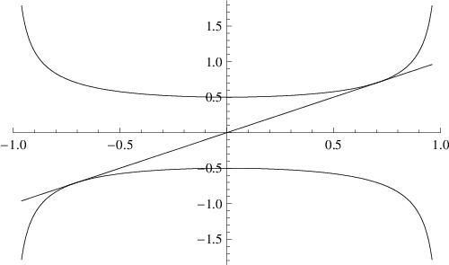
The estimating function is illustrated on Figure 1.
Refer to caption

Figure 1.

The tangent from oo to the graph of f⁡(z)=1/1−z2f(z)=1/\sqrt{1-z^{2}} has its contact point at z=1/2z=1/\sqrt{2}. Due to the convexity of f⁡(z)f(z), estimates (20) and (21) imply that if we choose the points x1,…,xd−1x_{1},\dots,x_{d-1} of norm about 1/21/\sqrt{2} with xd∈[o,x1,…,xd−1]x_{d}\in[o,x_{1},\dots,x_{d-1}], then M⁡(xd)M(x_{d}) is separated from [o,M⁡(x1),…,M⁡(xd)][o,M(x_{1}),\dots,M(x_{d})] by c​εc\varepsilon, where cc is a constant depending on dd only. This then yields a positive error 𝔼op​(K)\mathbb{E}^{p}_{o}(K) in comparison with 𝔼op​(Bd)\mathbb{E}^{p}_{o}(B^{d}). This idea is transformed to a quantitative proof as follows.

First, we estimate the decay of m⁡(x)m(x) around xdx_{d}. By convexity, [Bd,r]⊂K[B^{d},r\,]\subset K. Let r^=Sd−1∩[o,r]\hat{r}=S^{d-1}\cap[o\,,r\,], and r~=Sd−1∩([q​r]∖q)\tilde{r}=S^{d-1}\cap([q\,r\,]\setminus q). Estimate (20) yields that ‖r^−r~‖⩽ε\|\hat{r}-\tilde{r}\|\leqslant\varepsilon. For s∈Sd−1s\in S^{d-1}, denote by T⁡(s)T(s) be the tangent hyperplane to Sd−1S^{d-1} at ss. It is easily obtained that the intersection [Bd,r]∩T⁡(r^)[B^{d},r\,]\cap T(\hat{r}) is a (d−1)(d-1)-dimensional ball of radius ε/(2+ε)\sqrt{\varepsilon/(2+\varepsilon)}, and thus, A=[Bd,r]∩T⁡(r~)A=[B^{d},r\,]\cap T(\tilde{r}) contains a ball of radius ε/2.5\sqrt{\varepsilon/2.5} centred at r~\tilde{r}. Then, again by (20), πv​(A)\pi_{v}(A) contains a ball DD of radius ε/4\sqrt{\varepsilon}/4 centred at xdx_{d}. Since T⁡(q)T(q) is a tangent hyperplane of KK, m⁡(x)m(x) can be estimated over DD linearly:

(22) m⁡(xd+t​ε4​u)⩾(1−t)​m​(xd),∀u∈Sd−1,∀t∈[0,1].m\left(x_{d}+t\frac{\sqrt{\varepsilon}}{4}u\right)\geqslant(1-t)m(x_{d}),\ \forall\;u\in S^{d-1},\forall\;t\in[0,1].

Next, we are going to estimate 𝔼op​(K)−𝔼op​(Bd)\mathbb{E}^{p}_{o}(K)-\mathbb{E}_{o}^{p}(B^{d}). Let x0=ox_{0}=o, and choose x1,…,xd−1x_{1},\dots,x_{d-1} as follows. Take y~=xd/‖xd‖\tilde{y}=x_{d}/\|x_{d}\|. If d=2d=2, then let x1=y~/2x_{1}=\tilde{y}/\sqrt{2}. If d⩾3d\geqslant 3, then take y=(1/2−1/(100​d))​w~y=(1/\sqrt{2}-1/(100d))\tilde{w}, and let x1,…,xd−1x_{1},\dots,x_{d-1} be of norm 1/2−1/(500​d)1/\sqrt{2}-1/(500d), the vertices of a regular (d−2)(d-2)-simplex in (y+y⟂)∩H(y+y^{\perp})\cap H with centroid yy. Note that the distance between any two of these is >1/100​d>1/100\sqrt{d}. Let ϱ=1/(1000​d)\varrho=1/(1000d) and define Xi=xi+ϱ​Bd−1⊂HX_{i}=x_{i}+\varrho B^{d-1}\subset H for every i=1,…,d−1i=1,\dots,d-1. Then Vd−1​(Xi)≫1V_{d-1}(X_{i})\gg 1.

Note that by (20), there exists a neighbourhood UU of xdx_{d} of radius ≫ε\gg\sqrt{\varepsilon} in HH such that for any xi′∈Xi,i=1,…,d−1x_{i}^{\prime}\in X_{i},\ i=1,\dots,d-1, we have U⊂[o,x1′,…,xd−1′]U\subset[o,x_{1}^{\prime},\dots,x_{d-1}^{\prime}]. For such a collection of (xi′)(x_{i}^{\prime}), and for any xd′∈Ux_{d}^{\prime}\in U, define

D⁡((xi′))=D⁡(x1′,…,xd−1′,xd′)=[o,M⁡(x1′),…,M⁡(xd−1′)]∩σ⁡(xd′),D((x_{i}^{\prime}))=D(x_{1}^{\prime},\dots,x_{d-1}^{\prime},x_{d}^{\prime})=[o,M(x_{1}^{\prime}),\dots,M(x_{d-1}^{\prime})]\cap\sigma(x_{d}^{\prime}),

and let d⁡((xi′))=⟨D⁡((xi′)),v⟩d((x_{i}^{\prime}))=\langle D((x_{i}^{\prime})),v\rangle. Note that for any xi′∈Xix_{i}^{\prime}\in X_{i}, 1⩽i⩽d−11\leqslant i\leqslant d-1,

12−3500​d⩽‖xi′‖⩽12−1500​d.\frac{1}{\sqrt{2}}-\frac{3}{500d}\leqslant\|x_{i}^{\prime}\|\leqslant\frac{1}{\sqrt{2}}-\frac{1}{500d}.

Thus, (21) yields that there exists a neighbourhood V⊂UV\subset U of xdx_{d} in HH, still of area ≫ε(d−1)/2\gg\varepsilon^{(d-1)/2}, such that for any xi′∈Xix_{i}^{\prime}\in X_{i}, i=1,…,d−1i=1,\dots,d-1 and any xd′∈Vx_{d}^{\prime}\in V, for sufficiently small ε\varepsilon we have

(23) d⁡(x1′,…,xd′)⩽‖xd‖​ε1−1/(100​d).d(x_{1}^{\prime},\dots,x_{d}^{\prime})\leqslant\frac{\|x_{d}\|\varepsilon}{1-1/(100d)}.

Since

ε2​1−‖xd‖2−‖xd‖​ε1−1/(100​d)\frac{\varepsilon}{2\sqrt{1-\|x_{d}\|^{2}}}-\frac{\|x_{d}\|\varepsilon}{1-1/(100d)}

as a function of ‖xd‖\|x_{d}\| is decreasing for ‖xd‖<1/2\|x_{d}\|<1/\sqrt{2}, estimates (20), (21) and (23) yield that for xi′∈Xix_{i}^{\prime}\in X_{i} and xd′∈Vx_{d}^{\prime}\in V,

m⁡(xd)−d⁡(x1′,…,xd′)\displaystyle m(x_{d})-d(x_{1}^{\prime},\dots,x_{d}^{\prime}) ⩾ε⁡(12+1/(2​d)−1/2−1/(4​d)1−1/(100​d))\displaystyle\geqslant\varepsilon\left(\frac{1}{\sqrt{2}+1/(2\sqrt{d})}-\frac{1/\sqrt{2}-1/(4\sqrt{d})}{1-1/(100d)}\right)
⩾ε20​d.\displaystyle\geqslant\frac{\varepsilon}{20d}\;.

Let R=2​ε/(100​d)R=\sqrt{2\varepsilon}/(100d), and take Xd=V∩(xd+R​Bd−1)⊂HX_{d}=V\cap(x_{d}+RB^{d-1})\subset H. Then Vd−1​(Xd)≫ε(d−1)/2V_{d-1}(X_{d})\gg\varepsilon^{(d-1)/2}. Moreover, since m⁡(xd)<ε/2m(x_{d})<\varepsilon/\sqrt{2}, the above estimate and (22) yield that for xi′∈Xix_{i}^{\prime}\in X_{i}, i=1,…,di=1,\dots,d,

(24) m⁡(xd′)−d⁡((,,,,,))⩾ε100​d.m(x_{d}^{\prime})-d((x_{1}^{\prime},\dots,x_{d}^{\prime}))\geqslant\frac{\varepsilon}{100d}.

Let now K′K^{\prime} be the Steiner symmetral of KK with respect to HH. By Theorem 7, it is sufficient to prove that 𝔼op​(K)−𝔼op​(K′)⩾γ^p​ε(d+3)/2\mathbb{E}^{p}_{o}(K)-\mathbb{E}^{p}_{o}(K^{\prime})\geqslant\hat{\gamma}^{p}\varepsilon^{(d+3)/2}. We calculate the average volume of random simplices by integrating along the dd-tuples of chords of KK parallel to vv. For x∈Hx\in H, let σK​(x)=σ⁡(x)=K∩(x+ℓ)\sigma_{K}(x)=\sigma(x)=K\cap(x+\ell), and σK′​(x)=K′∩(x+ℓ)\sigma_{K^{\prime}}(x)=K^{\prime}\cap(x+\ell). For x1′,…,xd′∈H∩Kx_{1}^{\prime},\dots,x_{d}^{\prime}\in H\cap K, define

ω⁡(x1′,…,xd′)=∫σK​(x1′)…​∫σK​(xd′)V⁡[o,y1,…,yd]​d​yd​…​d​y1−∫σK′​(x1′)…∫σK′​(xd′)V[o,y1,…,yd]dyd…dy1\omega(x_{1}^{\prime},\dots,x_{d}^{\prime})=\int_{\sigma_{K}(x_{1}^{\prime})}\dots\int_{\sigma_{K}(x_{d}^{\prime})}V[o,y_{1},\dots,y_{d}]\,dy_{d}\dots dy_{1}\\ -\int_{\sigma_{K^{\prime}}(x_{1}^{\prime})}\dots\int_{\sigma_{K^{\prime}}(x_{d}^{\prime})}V[o,y_{1},\dots,y_{d}]\,dy_{d}\dots dy_{1}

Lemma 1 yields that for any (xi′)1d⊂H∩K(x^{\prime}_{i})_{1}^{d}\subset H\cap K, we have ω⁡(x1′,…,xd′)⩾0\omega(x_{1}^{\prime},\dots,x_{d}^{\prime})\geqslant 0. Moreover, by the construction of (Xi)1d−1(X_{i})_{1}^{d-1}, for any xi′∈Xix_{i}^{\prime}\in X_{i}, we have Vd−1​([o,x1′,…,xd−1′])≫1V_{d-1}([o,x_{1}^{\prime},\dots,x_{d-1}^{\prime}])\gg 1. Thus, by (24), Lemma 1, and part (i) of Lemma 2,

𝔼op​(K)−𝔼op​(K′)⩾∫X1…​∫Xdω⁡(x1′,…,xd′)​d​xd′​…​d​x1′⩾γ1p​ε(d+3)/2\mathbb{E}_{o}^{p}(K)-\mathbb{E}_{o}^{p}(K^{\prime})\geqslant\int_{X_{1}}\dots\int_{X_{d}}\omega(x_{1}^{\prime},\dots,x_{d}^{\prime})\,dx_{d}^{\prime}\dots dx_{1}^{\prime}\geqslant\gamma_{1}^{p}\varepsilon^{(d+3)/2}

for some γ1>0\gamma_{1}>0 depending only on dd.

Next, we estimate 𝔼d+1p​(K)−𝔼d+1p​(K′)\mathbb{E}^{p}_{d+1}(K)-\mathbb{E}^{p}_{d+1}(K^{\prime}). We start as before. There are two cases to be considered depending on ‖xd‖\|x_{d}\|. First, assume that ‖xd‖⩾1/100\|x_{d}\|\geqslant 1/100 (we need only ‖xd‖≫1\|x_{d}\|\gg 1). Then construct (Xi)1d(X_{i})_{1}^{d} as before. Choose R>0R>0 small enough such that the following hold:

  • i)

    For any x0′x^{\prime}_{0} with ‖x0′‖⩽R\|x_{0}^{\prime}\|\leqslant R, and any xi′∈Xix^{\prime}_{i}\in X_{i}, i=1,…,di=1,\dots,d, we have xd′∈[x0′,…,xd−1′]x^{\prime}_{d}\in[x^{\prime}_{0},\dots,x^{\prime}_{d-1}]

  • ii)

    For any x0′x^{\prime}_{0} with ‖x0′‖⩽R\|x_{0}^{\prime}\|\leqslant R and m⁡(x0′)⩽0m(x^{\prime}_{0})\leqslant 0, and any xi′∈Xix^{\prime}_{i}\in X_{i}, i=1,…,di=1,\dots,d,

    (25) m⁡(xd′)−⟨[M⁡(x0′),…,M⁡(xd−1′)]∩σ⁡(xd′),v⟩≫ε.m(x^{\prime}_{d})-\langle[M(x_{0}^{\prime}),\dots,M(x^{\prime}_{d-1})]\cap\sigma(x^{\prime}_{d}),v\rangle\gg\varepsilon.

Let X0={x∈H:|x|<R,m(x)⩽0}X_{0}=\{x\in H:|\,x|<R,\ m(x)\leqslant 0\}. By the symmetry of KK, the measure of X0X_{0} is at least half as large as that of R​Bd−1RB^{d-1}, thus, Vd−1​(X0)≫1V_{d-1}(X_{0})\gg 1. Then, part (ii) of Lemma 2 applies as before, yielding

𝔼d+1p​(K)−𝔼d+1p​(K′)⩾γ2p​ε(d+3)/2\mathbb{E}^{p}_{d+1}(K)-\mathbb{E}^{p}_{d+1}(K^{\prime})\geqslant\gamma_{2}^{p}\varepsilon^{(d+3)/2}

for some γ2>0\gamma_{2}>0 depending only on dd.

In the second case, xdx_{d} is close to the origin: ‖xd‖<1/100\|x_{d}\|<1/100. Let AA be the annulus {x∈H:1/2<‖x‖<3/4}\{x\in H:1/2<\|x\|<3/4\}. For this instance, define the function d′d^{\prime} on AdA^{d} by

d′​(x0′,…,xd−1′)=⟨([M⁡(x0′),…,M⁡(xd−1′)]∩σ⁡(o)),v⟩.d^{\prime}(x^{\prime}_{0},\dots,x^{\prime}_{d-1})=\langle([M(x^{\prime}_{0}),\dots,M(x^{\prime}_{d-1})]\cap\sigma(o)),v\rangle.

Note that by symmetry, d′​(−x0′,…,−xd−1′)=−d′​(x0′,…,xd−1′)d^{\prime}(-x^{\prime}_{0},\dots,-x^{\prime}_{d-1})=-d^{\prime}(x^{\prime}_{0},\dots,x^{\prime}_{d-1}). Let C=1/100C=1/100, and consider only those (xi′)0d−1⊂A(x^{\prime}_{i})_{0}^{d-1}\subset A, for which |⟨u,v⟩|⩾C|\langle u,v\rangle|\geqslant C, where uu is the normal vector of [M(x0′),…,M(xd−1′))][M(x^{\prime}_{0}),\dots,M(x^{\prime}_{d-1}))]. Then the (product) measure of these point sets is ≫1\gg 1; moreover, at least half of them satisfies d′​(x0′,…,xd−1′)⩽0d^{\prime}(x^{\prime}_{0},\dots,x^{\prime}_{d-1})\leqslant 0. These also satisfy (25). Thus, integrating over these sets, the argument works as before. ∎

Remark. In the planar case, one can obtain the following quantitative result: If KK satisfies the conditions of Lemma 2, then for small ε>0\varepsilon>0,

𝔼o1​(K)−𝔼o1​(B2)>ε5/2400.\mathbb{E}^{1}_{o}(K)-\mathbb{E}^{1}_{o}(B^{2})>\frac{\varepsilon^{5/2}}{400}\;.

From this, it also follows that if KK is a centrally symmetric convex disc, and 𝔼o1​(K)⩽(1+δ)​𝔼o1​(B2)\mathbb{E}^{1}_{o}(K)\leqslant(1+\delta)\mathbb{E}^{1}_{o}(B^{2}), then there exists an ellipse EE, for which E⊂K⊂(1+20​δ2/5)​EE\subset K\subset(1+20\delta^{2/5})E.

To obtain the estimate for not necessarily symmetric bodies, we cite the following result of the second author, see Theorem 1.4 of [10].

Lemma 4.

For any convex body K⊂ℝdK\subset\mathbb{R}^{d} with δBM​(K,Bd)>1+ε\delta_{\rm BM}(K,B^{d})>1+\varepsilon for some ε>0\varepsilon>0, there exists an oo-symmetric convex body CC with axial rotational symmetry and a constant γ>0\gamma>0 depending only on dd, such that δBM​(C,Bd)>γ​ε2\delta_{\rm BM}(C,B^{d})>\gamma\varepsilon^{2}, and CC results from KK as a limit of subsequent Steiner symmetrisations and affine transformations.

Now, we are ready to prove the general result.

Proof of Theorem 4.

Let δBM​(K,Bd)=1+δ\delta_{\rm BM}(K,B^{d})=1+\delta. By Lemma 4, we may assume that KK is an oo-symmetric convex body in John position, provided we prove

(26) 𝔼op​(K)\displaystyle\mathbb{E}^{p}_{o}(K) ⩾(1+γp​δd+32)​𝔼op​(Bd)​, and\displaystyle\geqslant(1+\gamma^{p}\delta^{\frac{d+3}{2}})\mathbb{E}^{p}_{o}(B^{d})\textrm{, and}
(27) 𝔼d+1p​(K)\displaystyle\mathbb{E}^{p}_{d+1}(K) ⩾(1+γp​δd+32)​𝔼d+1p​(Bd)\displaystyle\geqslant(1+\gamma^{p}\delta^{\frac{d+3}{2}})\mathbb{E}^{p}_{d+1}(B^{d})

for γ>0\gamma>0 depending only on dd. Let the maximal norm of points of KK be 1+ε1+\varepsilon. Since the volume of K∖BdK\setminus B^{d} is ≫ε(d+1)/2\gg\varepsilon^{(d+1)/2}, it follows that

(28) γ0​εd+12⩽δ⩽ε\gamma_{0}\varepsilon^{\frac{d+1}{2}}\leqslant\delta\leqslant\varepsilon

for γ0>0\gamma_{0}>0 depending only on dd.

Let ε0\varepsilon_{0} and γ^\hat{\gamma} come from Lemma 3. If δ⩽δ0=γ0​ε0d+12\delta\leqslant\delta_{0}=\gamma_{0}\varepsilon_{0}^{\frac{d+1}{2}} then ε⩽ε0\varepsilon\leqslant\varepsilon_{0} by (28), and hence we have (26) and (27) with γ=γ^\gamma=\hat{\gamma} by Lemma 3 and (28).

Therefore we may assume that δ>δ0\delta>\delta_{0}. Choose a sequence of Steiner symmetrals K0,K1,K2,…K_{0},K_{1},K_{2},\dots starting with K=K0K=K_{0} that converge to BdB^{d}, and hence there exists KnK_{n} such that δB​M​(Kn+1)⩽δ0<δB​M​(Kn)\delta_{BM}(K_{n+1})\leqslant\delta_{0}<\delta_{BM}(K_{n}). Let Lt:t∈[−1,1]L_{t}:t\in[-1,1] be the linear shadow system with L1=KnL_{1}=K_{n} and L0=Kn+1L_{0}=K_{n+1} corresponding to the Steiner symmetrisation of KnK_{n} (see Section 3), thus there exists t∈[0,1)t\in[0,1) such that δB​M​(Lt)=δ0\delta_{BM}(L_{t})=\delta_{0}. It follows that 𝔼∗p​(Lt)⩽𝔼∗p​(Kn)⩽𝔼∗p​(K)\mathbb{E}^{p}_{*}(L_{t})\leqslant\mathbb{E}^{p}_{*}(K_{n})\leqslant\mathbb{E}^{p}_{*}(K) and 𝔼d+1p​(Lt)⩽𝔼d+1p​(Kn)⩽𝔼d+1p​(K)\mathbb{E}^{p}_{d+1}(L_{t})\leqslant\mathbb{E}^{p}_{d+1}(K_{n})\leqslant\mathbb{E}^{p}_{d+1}(K), thus we conclude (26) and (27) by the previous case and δ<d\delta<\sqrt{d}. ∎

We made no attempt to find the best possible constants. However, the estimate ε(d+3)/2\varepsilon^{(d+3)/2} for centrally symmetric KK is close to the truth: if K=[r,−r,Bd]K=[r,-r,B^{d}], where rr is of norm 1+ε1+\varepsilon, then

𝔼op​(K)𝔼op​(Bd)−1≪ε(d+1)/2.\frac{\mathbb{E}^{p}_{o}(K)}{\mathbb{E}^{p}_{o}(B^{d})}-1\ll\varepsilon^{(d+1)/2.}

5. Stability of the maximum inequalities in the plane

Since here we work only on the plane, a convex disc means a planar convex body, and A​(K)=V2​(K)A(K)=V_{2}(K) is the area of KK. For a polygon Π\Pi with at least four vertices q1,…,qkq_{1},\ldots,q_{k} in this order, a basic linear shadow system at q1q_{1}, basic system for short, is defined as follows. Let q1′q^{\prime}_{1} and q1′′q^{\prime\prime}_{1} be points different from q1q_{1} such that q1∈[q1′,q1′′]q_{1}\in[q^{\prime}_{1},q^{\prime\prime}_{1}], q1′−q1′′q^{\prime}_{1}-q^{\prime\prime}_{1} is parallel to q2−qkq_{2}-q_{k}, and q2,…,qkq_{2},\ldots,q_{k} lie on the boundary of Π′=[q1′,q2,…,qk]\Pi^{\prime}=[q^{\prime}_{1},q_{2},\ldots,q_{k}] and Π′′=[q1′′,q2,…,qk]\Pi^{\prime\prime}=[q^{\prime\prime}_{1},q_{2},\ldots,q_{k}]. The corresponding basic system is the unique linear shadow system Πt\Pi_{t}, t∈[−β,α]t\in[-\beta,\alpha], such that α,β>0\alpha,\beta>0, α+β=1\alpha+\beta=1, Π−β=Π′′\Pi_{-\beta}=\Pi^{\prime\prime}, Π0=Π\Pi_{0}=\Pi, and Πα=Π′\Pi_{\alpha}=\Pi^{\prime}. In this case, the generating vector is parallel to q2−qkq_{2}-q_{k}, and the speed of any point in [q2,…,qk][q_{2},\ldots,q_{k}] is zero. It follows from Theorem 7 that for any n⩾3n\geqslant 3 and p⩾1p\geqslant 1,

(29) 𝔼p​(Π)<max⁡{𝔼p​(Π′),𝔼p​(Π′′)},\mathbb{E}^{p}(\Pi)<\max\{\mathbb{E}^{p}(\Pi^{\prime}),\mathbb{E}^{p}(\Pi^{\prime\prime})\},

where 𝔼p​(Π)\mathbb{E}^{p}(\Pi) stands either for 𝔼op​(Π)\mathbb{E}^{p}_{o}(\Pi) or 𝔼np​(Π)\mathbb{E}^{p}_{n}(\Pi). More precisely, the following holds:

(30) 𝔼p​(Π−t)\mathbb{E}^{p}(\Pi_{-t}) on [0,β][0,\beta], or 𝔼p​(Πt)\mathbb{E}^{p}(\Pi_{t}) on [0,α][0,\alpha], is strictly increasing.

For a convex disc KK, let TKT_{K} be a triangle of maximal area contained in KK. It follows that the triangle, the midpoints of whose sides are the vertices of TKT_{K}, contains KK. In particular, A⁡(K)<4​A​(TK)A(K)<4A(T_{K}).

First, we reduce the case to polygons with at most 6 vertices.

Proposition 2.

For a convex disc KK, let T~\widetilde{T} be the triangle, the midpoints of whose sides are the vertices of TKT_{K}. For n⩾3n\geqslant 3 and p⩾1p\geqslant 1, there exist polygons Π1\Pi_{1} and Π2\Pi_{2} with A⁡(Π1)=A⁡(Π2)=A⁡(K)A(\Pi_{1})=A(\Pi_{2})=A(K) such that TK⊂Π1,Π2T_{K}\subset\Pi_{1},\Pi_{2}, all vertices of Π1,Π2\Pi_{1},\Pi_{2} are on ∂T~\partial\widetilde{T}, and

𝔼np​(K)⩽𝔼np​(Π1)​ and ​𝔼∗p​(K)⩽𝔼∗p​(Π2).\mathbb{E}^{p}_{n}(K)\leqslant\mathbb{E}^{p}_{n}(\Pi_{1})\mbox{ \ and \ }\mathbb{E}^{p}_{*}(K)\leqslant\mathbb{E}^{p}_{*}(\Pi_{2}).
Proof.

We may assume that KK is not a triangle, and by continuity, that KK is a polygon. However, for k⩾4k\geqslant 4, suitable basic systems and (29) yield that among polygons PP of at most kk vertices with fixed area such that TK⊂P⊂T~T_{K}\subset P\subset\widetilde{T}, any polygon maximising either 𝔼np​(P)\mathbb{E}^{p}_{n}(P) or 𝔼∗p​(P)\mathbb{E}^{p}_{*}(P) has all of its vertices in ∂T~\partial\widetilde{T}. ∎

The core lemma comes.

Lemma 5.

There exist positive absolute constants ε0,c^\varepsilon_{0},\hat{c} such that if p⩾1p\geqslant 1, and A⁡(K)=(1+ε)​A​(TK)A(K)=(1+\varepsilon)A(T_{K}) for a convex disc KK and ε∈(0,ε0]\varepsilon\in(0,\varepsilon_{0}], then

𝔼3p​(K)⩽(1−c^p​ε2)​𝔼3p​(T2)​ and ​𝔼∗p​(K)⩽(1−c^p​ε2)​𝔼∗p​(T2).\mathbb{E}^{p}_{3}(K)\leqslant(1-\hat{c}^{p}\varepsilon^{2})\mathbb{E}^{p}_{3}(T^{2})\mbox{ \ and \ }\mathbb{E}^{p}_{*}(K)\leqslant(1-\hat{c}^{p}\varepsilon^{2})\mathbb{E}^{p}_{*}(T^{2}).
Proof.

We first consider 𝔼∗p​(K)\mathbb{E}^{p}_{*}(K). Let TK=[p1,p2,p3]T_{K}=[p_{1},p_{2},p_{3}], and let q1,q2,q3q_{1},q_{2},q_{3} be the such that pip_{i} is the midpoint of [qj,qk][q_{j},q_{k}], {i,j,k}={1,2,3}\{i,j,k\}=\{1,2,3\}. We may assume that each side of TKT_{K} is of length one, and γ⁡(TK)=o\gamma(T_{K})=o.

Let Π\Pi be the polygon provided by Claim 2, and let xx be the farthest vertex of Π\Pi from TKT_{K}. We may assume that x∈[p1,q2]x\in[p_{1},q_{2}]. It follows that A⁡([x,p1,p3])A([x,p_{1},p_{3}]) is between ε​A​(TK)/6\varepsilon A(T_{K})/6 and ε​A​(TK)\varepsilon A(T_{K}), and hence

(31) ε/6⩽‖x−p1‖⩽ε.\varepsilon/6\leqslant\|x-p_{1}\|\leqslant\varepsilon.

Let us number the vertices of Π\Pi in such a way that x=x3x=x_{3}, its neighbouring vertices are x2∈[p1,q3]x_{2}\in[p_{1},q_{3}] and x4∈[p3,q2]x_{4}\in[p_{3},q_{2}], and the other neighbours of x2x_{2} and x4x_{4} are x1∈[p2,q3]x_{1}\in[p_{2},q_{3}] and x5x_{5}, respectively; see Figure 2. Here possibly x5=x1x_{5}=x_{1}, and either x5∈[p3,q1]x_{5}\in[p_{3},q_{1}], or x5∈[p2,q1]x_{5}\in[p_{2},q_{1}]. The definition of x=x3x=x_{3} yields that for any i=1,2,4,5i=1,2,4,5 there exists j∈{1,2,3}j\in\{1,2,3\} such that

(32) ‖xi−pj‖⩽‖x−p1‖.\|x_{i}-p_{j}\|\leqslant\|x-p_{1}\|.

To deform Π\Pi, let ll be the line parallel to x2−x4x_{2}-x_{4} passing through xx, and let x′x^{\prime} and x′′x^{\prime\prime} be the intersections of ll with aff​{x2,x1}{\rm aff}\{x_{2},x_{1}\} and aff​{x4,x5}{\rm aff}\{x_{4},x_{5}\}, respectively. We consider the basic system Πt\Pi_{t}, t∈[−β,α]t\in[-\beta,\alpha], α,β>0\alpha,\beta>0, α+β=1\alpha+\beta=1, where Π0=Π\Pi_{0}=\Pi, x′x^{\prime} is a vertex of Πα\Pi_{\alpha}, and x′′x^{\prime\prime} is a vertex of Π−β\Pi_{-\beta}. We write φ⁡(z)\varphi(z) to denote the speed of a z∈Πz\in\Pi, and observe that the generating vector is v=x2−x4‖x2−x4‖v=\frac{x_{2}-x_{4}}{\|x_{2}-x_{4}\|}.

Refer to caption

Figure 2.

It follows by (15) that γ⁡(Π)=β​γ​(Πα)+α​γ​(Π−β)\gamma(\Pi)=\beta\,\gamma(\Pi_{\alpha})+\alpha\,\gamma(\Pi_{-\beta}). Thus for any z1,z2∈Πz_{1},z_{2}\in\Pi, Theorem 6 yields

(33) A​([γ⁡(Π),z1,z2])p⩽β​A​([γ⁡(Πα),z1+α​φ​(z1)​v,z2+α​φ​(z2)​v])p+α​A​([γ⁡(Π−β),z1−β​φ​(z1)​v,z2−β​φ​(z2)​v])p.A([\gamma(\Pi),z_{1},z_{2}])^{p}\leqslant\beta A([\gamma(\Pi_{\alpha}),z_{1}+\alpha\varphi(z_{1})v,z_{2}+\alpha\varphi(z_{2})v])^{p}\\ +\alpha A([\gamma(\Pi_{-\beta}),z_{1}-\beta\varphi(z_{1})v,z_{2}-\beta\varphi(z_{2})v])^{p}.

In order to obtain a stability statement, we improve on (33). As a first step, we localise γ⁡(Πt)\gamma(\Pi_{t}). The centroid γ⁡(Π)\gamma(\Pi) has the property that −1/3(Π−γ(Π))⊂Π−γ(Π)-1/3\,(\Pi-\gamma(\Pi))\subset\Pi-\gamma(\Pi). It follows by (31) and (32) that

(34) γ⁡(Π)∈2​ε​TK.\gamma(\Pi)\in 2\varepsilon T_{K}.

We note that by (32), |φ⁡(z)|⩽1.1|\varphi(z)|\leqslant 1.1 for z∈Πz\in\Pi, and φ⁡(z)=0\varphi(z)=0 if zz is separated from x=x3x=x_{3} by the diagonal [x2,x4][x_{2},x_{4}]. Thus (15) yields

(35) γ(Πt)=γ(Π)+tωv, for ω∈(0,2​ε) independent of t.\gamma(\Pi_{t})=\gamma(\Pi)+t\omega v,\mbox{ \ for $\omega\in(0,2\varepsilon)$ independent of $t$.}

As [p1,p3][p_{1},p_{3}] is close to ll (any z∈[p1,p2]z\in[p_{1},p_{2}] is of distance at most 3​ε3\varepsilon from ll) and [p1,p2][p_{1},p_{2}] is close to [x2,x1][x_{2},x_{1}], we may choose ε0\varepsilon_{0} small enough to ensure ε/12⩽‖x−x′‖⩽2​ε\varepsilon/12\leqslant\|x-x^{\prime}\|\leqslant 2\varepsilon. In addition, [x4,x5][x_{4},x_{5}] is either contained in [q2,q1][q_{2},q_{1}], or it is close to [p3,p2][p_{3},p_{2}], therefore 2/3⩽‖x−x′′‖⩽3/22/3\leqslant\|x-x^{\prime\prime}\|\leqslant 3/2. We deduce

(36) ε/24⩽α⩽4​ε.\varepsilon/24\leqslant\alpha\leqslant 4\varepsilon.

We may assume that ℝ=v⊥\mathbb{R}=v^{\bot}, oriented in a way such that πv​p3>0\pi_{v}p_{3}>0. We observe that

12​3−ε<πv​p3⩽12​3⩽πv​p1<πv​x3−ε12.\frac{1}{2\sqrt{3}}-\varepsilon<\pi_{v}p_{3}\leqslant\frac{1}{2\sqrt{3}}\leqslant\pi_{v}p_{1}<\pi_{v}x_{3}-\frac{\varepsilon}{12}.

For y∈πv​int​Πy\in\pi_{v}{\rm int}\Pi and t∈[−β,α]t\in[-\beta,\alpha], we write σt​(y)\sigma_{t}(y) to denote the chord of Πt\Pi_{t} parallel to vv and projecting into yy, and mt​(y)m_{t}(y) to denote the midpoint of σt​(y)\sigma_{t}(y). In particular, σt​(y)=σ0​(y)\sigma_{t}(y)=\sigma_{0}(y) if y⩽πv​x2y\leqslant\pi_{v}x_{2}. If ε0\varepsilon_{0} is small enough then for any s∈(0,18)s\in(0,\frac{1}{8}),

|⟨v,m(πvp3−s)⟩|⩽2s and V1​(σ​(y))>32.|\langle v,m(\pi_{v}p_{3}-s)\rangle|\leqslant 2s\mbox{ and $V_{1}(\sigma(y))>\frac{\sqrt{3}}{2}$.}

We consider the intervals

I1=[πv​p3−116,πv​p3−132] and I2=[116​πv​p1+1516​πv​x3,132​πv​p1+3132​πv​x3],\mbox{$I_{1}=[\pi_{v}p_{3}-\frac{1}{16},\pi_{v}p_{3}-\frac{1}{32}]$ and $I_{2}=[\frac{1}{16}\pi_{v}p_{1}+\frac{15}{16}\pi_{v}x_{3},\frac{1}{32}\pi_{v}p_{1}+\frac{31}{32}\pi_{v}x_{3}]$},

and hence (31) yields

(37) V1​(I1)=132 and V1​(I2)⩾ε12⋅64.\mbox{$V_{1}(I_{1})=\frac{1}{32}$ and $V_{1}(I_{2})\geqslant\frac{\varepsilon}{12\cdot 64}$}.

In addition, σt​(y)=σ0​(y)\sigma_{t}(y)=\sigma_{0}(y) if y∈I1y\in I_{1} and t∈[−β,α]t\in[-\beta,\alpha]. To ensure the condition (18) in Lemma 2, for y∈I1y\in I_{1}, we restrict our attention to

σt∗​(y)=18​(σt​(y)−mt​(y))+mt​(y).\sigma^{*}_{t}(y)=\mbox{$\frac{1}{8}$}(\sigma_{t}(y)-m_{t}(y))+m_{t}(y).

Our main claim is that there exists an absolute constant c1>0c_{1}>0, such that for any y1∈I1y_{1}\in I_{1} and y2∈I2y_{2}\in I_{2}, the integral

f⁡(t)=∫σt∗​(y1)∫σt​(y2)A​([γ⁡(Πt),z1,z2])p​d​z1​d​z2f(t)=\int_{\sigma^{*}_{t}(y_{1})}\int_{\sigma_{t}(y_{2})}A([\gamma(\Pi_{t}),z_{1},z_{2}])^{p}\,dz_{1}dz_{2}

satisfies

(38) α​f​(−β)+β​f​(α)⩾f⁡(0)+c1p​ε.\alpha f(-\beta)+\beta f(\alpha)\geqslant f(0)+c_{1}^{p}\varepsilon.

It follows by (34) and (35) that if ε0\varepsilon_{0} is small enough, then there exists a τ∈(14,34)\tau\in(\frac{1}{4},\frac{3}{4}), such that γ⁡(Π−τ)\gamma(\Pi_{-\tau}), m−τ​(y1)m_{-\tau}(y_{1}) and m−τ​(y2)m_{-\tau}(y_{2}) are collinear. Writing ωt\omega_{t} to denote the intersection point of aff⁡{γ⁡(Πt),mt​(y1)}{\rm aff}\{\gamma(\Pi_{t}),m_{t}(y_{1})\} and aff​σt​(y2){\rm aff}\sigma_{t}(y_{2}), the function ⟨v,ωt−mt​(y2)⟩\langle v,\omega_{t}-m_{t}(y_{2})\rangle of tt is linear, zero at −τ-\tau, and satisfies

⟨v,ωα−mα​(y2)⟩⩾18 and ⟨v,ω−β−m−β​(y2)⟩⩽−18.\mbox{$\langle v,\omega_{\alpha}-m_{\alpha}(y_{2})\rangle\geqslant\frac{1}{8}$ and $\langle v,\omega_{-\beta}-m_{-\beta}(y_{2})\rangle\leqslant-\frac{1}{8}$}.

We deduce by Lemma 1 and (16) that f⁡(t)f(t) is convex, and has its minimum at −τ-\tau. Thus Lemma 2 yields

f(α),f(−β)⩾f(−τ)+c2p for an absolute constant c2>0.f(\alpha),f(-\beta)\geqslant f(-\tau)+c_{2}^{p}\mbox{ \ for an absolute constant $c_{2}>0$.}

It follows by β=1−α\beta=1-\alpha and (36) that

α​f​(−β)+β​f​(α)−f⁡(0)\displaystyle\alpha f(-\beta)+\beta f(\alpha)-f(0) ⩾α​f​(−β)+β​f​(α)−αα+τ​f​(−τ)−τα+τ​f​(α)\displaystyle\geqslant\alpha f(-\beta)+\beta f(\alpha)-\mbox{$\frac{\alpha}{\alpha+\tau}\,f(-\tau)-\frac{\tau}{\alpha+\tau}\,f(\alpha)$}
=α​f​(−β)+α⋅1−α−τα+τ​f​(α)−αα+τ​f​(−τ)\displaystyle=\alpha f(-\beta)+\mbox{$\alpha\cdot\frac{1-\alpha-\tau}{\alpha+\tau}\,f(\alpha)-\frac{\alpha}{\alpha+\tau}\,f(-\tau)$}
⩾αα+τ⋅c2p⩾c2p24⋅ε.\displaystyle\geqslant\mbox{$\frac{\alpha}{\alpha+\tau}\cdot c_{2}^{p}\geqslant\frac{c_{2}^{p}}{24}\cdot\varepsilon$}.

Therefore we have verified (38). In turn combining this with (33) and (37) proves for a suitable absolute constant c3>0c_{3}>0, that

𝔼∗p​(Π)+c3p​ε2⩽β​𝔼∗p​(Πα)+α​𝔼∗p​(Π−β)⩽max⁡{𝔼∗p​(Πα),𝔼∗p​(Π−β)}.\mathbb{E}^{p}_{*}(\Pi)+c_{3}^{p}\varepsilon^{2}\leqslant\beta\mathbb{E}^{p}_{*}(\Pi_{\alpha})+\alpha\mathbb{E}^{p}_{*}(\Pi_{-\beta})\leqslant\max\{\mathbb{E}^{p}_{*}(\Pi_{\alpha}),\mathbb{E}^{p}_{*}(\Pi_{-\beta})\}.

Applying subsequent basic systems to the one of Πα\Pi_{\alpha} and Π−β\Pi_{-\beta} with larger 𝔼∗p​(⋅)\mathbb{E}^{p}_{*}(\cdot), we conclude

𝔼∗p​(K)+c3p​ε2⩽𝔼∗p​(Π)+c3p​ε2⩽𝔼∗p​(T2).\mathbb{E}^{p}_{*}(K)+c_{3}^{p}\varepsilon^{2}\leqslant\mathbb{E}^{p}_{*}(\Pi)+c_{3}^{p}\varepsilon^{2}\leqslant\mathbb{E}^{p}_{*}(T^{2}).

Turning to 𝔼3p​(K)\mathbb{E}^{p}_{3}(K), the major difference of the argument is that we need a third interval for the third vertex of the triangle. Writing I1=[a,b]I_{1}=[a,b], we define I~2=I2\widetilde{I}_{2}=I_{2}, and

I~0=a+110​(I1−a) and I~1=b+110​(I1−b).\mbox{$\widetilde{I}_{0}=a+\frac{1}{10}(I_{1}-a)$ and $\widetilde{I}_{1}=b+\frac{1}{10}(I_{1}-b)$}.

In addition, we shorten σt∗​(y)\sigma^{*}_{t}(y) for y∈I1y\in I_{1} to

σ~t​(y)=180​(σt​(y)−mt​(y))+mt​(y).\tilde{\sigma}_{t}(y)=\mbox{$\frac{1}{80}$}(\sigma_{t}(y)-m_{t}(y))+m_{t}(y).

We change our main claim (38) to the following. There exists an absolute constant c4>0c_{4}>0, such that for any y0∈I~0y_{0}\in\widetilde{I}_{0}, y1∈I~1y_{1}\in\widetilde{I}_{1} and y2∈I~2y_{2}\in\widetilde{I}_{2}, the integral

f~​(t)=∫σ~t​(y0)∫σ~t​(y1)∫σt​(y2)A​([z0,z1,z2])p​d​z0​d​z1​d​z2\tilde{f}(t)=\int_{\tilde{\sigma}_{t}(y_{0})}\int_{\tilde{\sigma}_{t}(y_{1})}\int_{\sigma_{t}(y_{2})}A([z_{0},z_{1},z_{2}])^{p}\,dz_{0}dz_{1}dz_{2}

satisfies

(39) α​f~​(−β)+β​f~​(α)⩾f~​(0)+c4p​ε.\alpha\tilde{f}(-\beta)+\beta\tilde{f}(\alpha)\geqslant\tilde{f}(0)+c_{4}^{p}\varepsilon.

Now the proof of Lemma 5 can be completed along the argument above by introducing the obvious alterations. ∎

Corollary 1.

There exists a positive absolute constant c~\tilde{c} such that if p⩾1p\geqslant 1, and A⁡(K)=(1+ε)​A​(TK)A(K)=(1+\varepsilon)A(T_{K}) for a convex disc KK, then

𝔼3p​(K)⩽(1−c~p​ε2)​𝔼3p​(T2)​ and ​𝔼∗p​(K)⩽(1−c~p​ε2)​𝔼∗p​(T2).\mathbb{E}^{p}_{3}(K)\leqslant(1-\tilde{c}^{p}\varepsilon^{2})\mathbb{E}^{p}_{3}(T^{2})\mbox{ \ and \ }\mathbb{E}^{p}_{*}(K)\leqslant(1-\tilde{c}^{p}\varepsilon^{2})\mathbb{E}^{p}_{*}(T^{2}).
Proof.

We present the argument only for 𝔼3p​(K)\mathbb{E}^{p}_{3}(K). Let c^\hat{c} and ε0\varepsilon_{0} come from Lemma 5. We may assume that KK is an mm-gon for m⩾4m\geqslant 4 by continuity, and that A⁡(K)>(1+ε0)​A​(TK)A(K)>(1+\varepsilon_{0})A(T_{K}) by Lemma 5. It follows by (30), that there exist m−3m-3 consecutive basic systems that induce a continuous deformation of KK into a triangle in a way such that 𝔼3p​(⋅)\mathbb{E}^{p}_{3}(\cdot) is strictly increasing during the deformation. Therefore there exists a polygon K′K^{\prime} such that 𝔼3p​(K′)>𝔼3p​(K)\mathbb{E}^{p}_{3}(K^{\prime})>\mathbb{E}^{p}_{3}(K), and A⁡(K′)=(1+ε0)​A​(TK′)A(K^{\prime})=(1+\varepsilon_{0})A(T_{K^{\prime}}). Now we apply Lemma 5 to K′K^{\prime}, and using ε<3\varepsilon<3, we deduce

𝔼3p​(K)<𝔼3p​(K′)⩽(1−c^p​ε02)​𝔼3p​(T2)<(1−c^p​ε029⋅ε2)​𝔼3p​(T2).∎\mathbb{E}^{p}_{3}(K)<\mathbb{E}^{p}_{3}(K^{\prime})\leqslant(1-\hat{c}^{p}\varepsilon_{0}^{2})\mathbb{E}^{p}_{3}(T^{2})<\mbox{$(1-\frac{\hat{c}^{p}\varepsilon_{0}^{2}}{9}\cdot\varepsilon^{2})\mathbb{E}^{p}_{3}(T^{2})$}.\qed

Having Corollary 1, Theorem 5 is a consequence of the following.

Lemma 6.

If δB​M​(K,T2)=1+δ\delta_{BM}(K,T^{2})=1+\delta for a convex disc KK, then

(1+δ)​A​(TK)⩽A⁡(K)<(1+δ)2​A​(TK).(1+\delta)A(T_{K})\leqslant A(K)<(1+\delta)^{2}A(T_{K}).
Proof.

The upper bound is consequence of the fact that by the definition of the Banach-Mazur distance, there exists a triangle T′⊂KT^{\prime}\subset K, and x∈T′x\in T^{\prime}, such that K⊂(1+δ)​(T′−x)+xK\subset(1+\delta)(T^{\prime}-x)+x. For the lower bound, we may assume that TKT_{K} is a regular triangle of edge length one. Let p1,p2,p3p_{1},p_{2},p_{3} be the vertices of TKT_{K}, and let q1,q2,q3q_{1},q_{2},q_{3} be the such that pip_{i} is the midpoint of [qj,qk][q_{j},q_{k}], {i,j,k}={1,2,3}\{i,j,k\}=\{1,2,3\}. If {i,j,k}={1,2,3}\{i,j,k\}=\{1,2,3\}, then let tit_{i} be the maximal distance of points of K∩[qi,pj,pk]K\cap[q_{i},p_{j},p_{k}] from [pj,pk][p_{j},p_{k}]. On the one hand,

A⁡(K)⩾A⁡(TK)+(t1+t2+t3)/2=(1+23​(t1+t2+t3))​A​(TK).A(K)\geqslant A(T_{K})+(t_{1}+t_{2}+t_{3})/2=\mbox{$(1+\frac{2}{\sqrt{3}}(t_{1}+t_{2}+t_{3}))$}A(T_{K}).

On the other hand, KK is contained in a regular triangle, that is similarly situated to TKT_{K}, and whose height is 32+t1+t2+t3\frac{\sqrt{3}}{2}+t_{1}+t_{2}+t_{3}. It follows that

1+δ⩽(32+t1+t2+t3)/32=1+23​(t1+t2+t3)⩽A⁡(K)/A⁡(TK).∎1+\delta\leqslant\mbox{$(\frac{\sqrt{3}}{2}+t_{1}+t_{2}+t_{3})/\frac{\sqrt{3}}{2}=1+\frac{2}{\sqrt{3}}(t_{1}+t_{2}+t_{3})$}\leqslant A(K)/A(T_{K}).\qed

That the exponent 22 in the error term δ2\delta^{2} is optimal is shown by the example of the closure of T\δ​TT\backslash\delta T, where TT is a triangle such that oo is a vertex.

6. Stability of Petty projection inequality

Theorem 1 readily implies the stability version of the Busemann-Petty centroid inequality (5), using (4). Here we also derive the stability version of Petty’s projection inequality (cf. [33]). Given a convex body KK, its projection body Π​K\Pi K is defined by its support function

hΠ​K​(u)=Vd−1​(pu​(K)).h_{\Pi K}(u)=V_{d-1}(p_{u}(K)).

The Petty projection inequality states that the quantity

Vd​(K)d−1​Vd​(Π∗​(K))V_{d}(K)^{d-1}V_{d}(\Pi^{*}(K))

is maximised for ellipsoids. Citing formula (5.7) of [33] and using (4), we arrive to that if Vd​(K)=1V_{d}(K)=1, then

(40) 1Vd​(K)d−1​Vd​(Π∗​K)⩾(d+12)d​Vd​(Γ⁡(Π∗​K))Vd​(Π∗​K)=(d+1)d​𝔼o1​(Π∗​K).\frac{1}{V_{d}(K)^{d-1}V_{d}(\Pi^{*}K)}\geqslant\left(\frac{d+1}{2}\right)^{d}\frac{V_{d}(\Gamma(\Pi^{*}K))}{V_{d}(\Pi^{*}K)}=(d+1)^{d}\mathbb{E}^{1}_{o}(\Pi^{*}K).

Let δB​M​(K,Bd)=1+δ\delta_{BM}(K,B^{d})=1+\delta. Bourgain and Lindenstrauss [12] proved that there exists a constant CC depending on dd, so that

δB​M​(Π​K,Bd)⩾1+C​δ(d2+5​d)/2.\delta_{BM}(\Pi K,B^{d})\geqslant 1+C\delta^{(d^{2}+5d)/2}.

Referring to δB​M​(Π​K,Bd)=δB​M​(Π∗​K,Bd)\delta_{BM}(\Pi K,B^{d})=\delta_{BM}(\Pi^{*}K,B^{d}), Theorem 1 implies that there exists a constant cc depending on dd only, so that

𝔼o1​(Π∗​K)⩾(1+C′​δd​(d+3)​(d+5)/2)​𝔼o1​(Bd).\mathbb{E}^{1}_{o}(\Pi^{*}K)\geqslant(1+C^{\prime}\delta^{d(d+3)(d+5)/2})\mathbb{E}^{1}_{o}(B^{d}).

Thus, from (40) we obtain that

Vd​(K)d−1​Vd​(Π∗​K)⩽(1+c​δd​(d+3)​(d+5)/2)−1​Vd​(Bd)d−1​Vd​(Π∗​Bd).V_{d}(K)^{d-1}V_{d}(\Pi^{*}K)\leqslant(1+c\delta^{d(d+3)(d+5)/2})^{-1}V_{d}(B^{d})^{d-1}V_{d}(\Pi^{*}B^{d}).

We note that the stability version of the Busemann intersection inequality (3) would also follow by verifying a statement of the following type. If KK is a convex body in ℝd\mathbb{R}^{d}, and δB​M​(K,Bd)=1+δ\delta_{BM}(K,B^{d})=1+\delta for some δ>0\delta>0, then there exist ν,η>0\nu,\eta>0 (depending on δ\delta) so that δB​M​(K∩u⟂,Bd−1)>1+η\delta_{BM}(K\cap u^{\perp},B^{d-1})>1+\eta for a set of directions uu of measure at least ν\nu. The enthusiast would believe in such a statement with an absolute constant ν\nu and η=δq\eta=\delta^{q} for some q>0q>0.

7. Acknowledgements

We would like to thank Imre Bárány for drawing our attention to the problem and for useful comments, and Ferenc Fodor, Vitali Milman and Alain Pajor for the valuable suggestions and enlightening discussions.

References

  • [1] K.M. Ball: Logarithmically concave functions and sections of convex sets in ℝn\mathbb{R}^{n}. Studia Math., 88 (1988), 69–84.
  • [2] K.M. Ball: An elementary introduction to modern convex geometry. In: Flavors of convex geometry, ed. S. Levy, Cambridge University Press, Cambridge, 1997.
  • [3] I. Bárány: Random points and lattice points in convex bodies. Bull. Amer. Math. Soc. (N.S.) 45 (2008), no. 3, 339–365.
  • [4] I. Bárány, C. Buchta: Random polytopes in a convex polytope, independence of shape, and concentration of vertices. Math. Annalen, 297 (1993), 467-497.
  • [5] T. Bisztriczky, K.J. Böröczky: About the centroid body and the ellipsoid of inertia. Mathematika 48 (2001), 1-13 (2003).
  • [6] W. Blaschke: Über affine Geometrie IX: Verschiedene Bemerkungen un Aufgaben. Ber. Verh. Sächs. Akad. Wiss. Leipzig Math.–Phys. Kl., 69 (1917), 412-420.
  • [7] W. Blaschke: Über affine Geometrie XI: eine minimum Aufgabe für Legendres trägheits Ellipsod. Ber. Verh. Sächs. Akad. Wiss. Leipzig Math.–Phys. Kl., 70 (1918), 72-75.
  • [8] W. Blaschke: Vorlesungen über Differentialgeometrie II: Affine Differentialgeometrie. Springer, Berlin, 1923.
  • [9] T. Bonnesen, W. Fenchel: Theorie der konvexen Körper. Springer, Berlin, 1934. English translation: Theory of convex bodies. BCS Associates, Moscow, Idaho, U.S.A., 1987.
  • [10] K.J. Böröczky: Stability of the Blaschke-Santaló and the affine isoperimetric inequality. Adv. Math., accepted.
  • [11] J. Bourgain: On high-dimensional maximal functions associated to convex bodies. Amer. J. Math., 108 (1986), 1467–1476.
  • [12] J. Bourgain, J. Lindenstrauss: Projection bodies. Geometric aspects of functional analysis (1986), Lecture Notes in Math., 1317, Springer, Berlin, 1988, 250–270.
  • [13] J. Bourgain, M. Meyer, V. Milman, A. Pajor: On a geometric inequality. Geometric aspects of functional analysis (1986/87), Lecture Notes in Math., 1317, Springer, Berlin, 1988, 271–282.
  • [14] C. Buchta: Zufallspolygone in konvexen Vielecken. J. reine angew. Math., 347 (1984), 212–220.
  • [15] C. Buchta, M. Reitzner: The convex hull of random points in a tetrahedron: Solution of Blaschke’s problem and more general results. J. reine angew. Math., 536 (2001), 1-29.
  • [16] H. Busemann: Volume in terms of concurrent cross–sections. Pacific J. Math., 3 (1953), 1-12.
  • [17] S. Campi, A. Colesanti, P. Gronchi: A note on Sylvester’s problem for random polytopes in a convex body. Rendiconti dell’Istituto di Matematica dell’Universitiá di Trieste, 31 (1999), 1-16.
  • [18] S. Campi, P. Gronchi: Volume inequalities for LpL_{p}-zonotopes. Mathematika 53 (2006), no. 1, 71-80 (2007).
  • [19] L. Dalla, D.G. Larman: Volumes of a random polytope in a convex set. Applied geometry and discrete mathematics, DIMACS Ser. Discrete Math. Theoret. Comput. Sci., 4, Amer. Math. Soc., Providence, RI, 1991, 17–180.
  • [20] B. Fleury, O. Guédon, G. Paouris: A stability result for mean width of LpL_{p}-centroid bodies. Adv. Math. 214 (2007), no. 2, 865-877.
  • [21] H. Hadwiger: Vorlesungen über Inhalt, Oberfläche und Isoperimetrie. Springer-Verlag, Berlin-Göttingen-Heidelberg, 1957.
  • [22] A. Giannopoulos: On the mean value of the area of a random polygon in a plane convex body. Mathematika 39 (1992), 279-290.
  • [23] A. Giannopoulos: Notes on Isotropic Convex Bodies. Preprint. http://users.uoa.gr/∼\simapgiannop/
  • [24] A. Giannopoulos, V.D. Milman: Asymptotic convex geometry: short overview. Different faces of geometry, Int. Math. Ser. (N. Y.), Kluwer/Plenum, New York, 2004, 87-162.
  • [25] R.J. Gardner: Geometric Tomography (2nd ed.) Cambridge University Press, Cambridge, 2006.
  • [26] H. Groemer: On some mean values associated with a randomly selected simplex in a convex set. Pacific J. Math. 45 (1973), 525–533.
  • [27] H. Groemer: On the mean value of the volume of a random polytope in a convex set. Arch. Math., 25 (1974), 86-90.
  • [28] H. Groemer: Stability theorems for ellipsoids and spheres. J. London Math. Soc. (2), 49 (1994), 357-370.
  • [29] P.M. Gruber: Convex and discrete geometry. Springer, Berlin, 2007.
  • [30] F. John: Extremum problems with inequalities as subsidiary conditions. Courant Anniversary Volume, Interscience, New York, 1948, 187–204.
  • [31] V. Klee: What is the expected volume of a simplex whose vertices are chosen at random from a given convex body. Amer. Math. Monthly, 76 (1969), 186–188.
  • [32] J. Lagarias, G. Ziegler: Bounds for lattice polytopes containing a fixed number of interior points in a sublattice. Canad. J. Math., 43 (1991), 1022–1035.
  • [33] E. Lutwak: Selected affine isoperimetric inequalities. In: Handbook of convex geometry A, 151–176. North-Holland, Amsterdam, 1993.
  • [34] M. Meyer, S. Reisner: Shadow systems and volumes of polar convex bodies. Mathematika, 53 (2006), 129–148.
  • [35] V.D. Milman, A. Pajor: Isotropic position and inertie ellipsoids and zonoids of the unit ball of a normed nn–dimensional space. Geometric Aspects of Functional Analysis, ed. J. Lindenstrauss and V.D. Milman, Lec. Notes Math. 1376 Springer, (1989), 64–104.
  • [36] C.M. Petty: Centroid surfaces. Pacific J. Math., 11 (1961), 1535–1547.
  • [37] W.J. Reed: Random points in a simplex. Pacific J. Math., 54, 183–198 (1974)
  • [38] C.A. Rogers, G.C. Shephard: Some extremal problems for convex bodies. Mathematika 5 (1958), 93–102.
  • [39] R. Schneider: Convex Bodies: The Brunn-Minkowski Theory. Cambridge University Press, 1993.
  • [40] R. Schneider, W. Weil: Stochastic and Integral Geometry. Springer-Verlag, 2008.
  • [41] G.C. Shephard: Shadow systems of convex bodies. Israel J. Math., 2 (1964), 229-36.
  • [42] J. J. Sylvester: Problem 1491. The Educational Times (April 1864), London.