Spectral Shape of Check-Hybrid GLDPC Codes
Abstract
This paper analyzes the asymptotic exponent of both the weight spectrum and the stopping set size spectrum for a class of generalized low-density parity-check (GLDPC) codes. Specifically, all variable nodes (VNs) are assumed to have the same degree (regular VN set), while the check node (CN) set is assumed to be composed of a mixture of different linear block codes (hybrid CN set). A simple expression for the exponent (which is also referred to as the growth rate or the spectral shape) is developed. This expression is consistent with previous results, including the case where the normalized weight or stopping set size tends to zero. Furthermore, it is shown how certain symmetry properties of the local weight distribution at the CNs induce a symmetry in the overall weight spectral shape function.
I Introduction
Tanner codes were introduced in [1] as a generalization of Gallager’s low-density parity-check (LDPC) codes [2]. In the bipartite graph representation of a Tanner code, all variable nodes (VNs) have the same degree and may be interpreted as repetition codes with the same length (regular VN set). Moreover, all check nodes (CNs) are generic linear block codes with the same length, dimension and code book (regular CN set). Tanner codes with an irregular VN set (i.e., VNs with different degrees) or with a hybrid CN set (i.e., CNs of different types) are more generically referred to as generalized LDPC (GLDPC) codes in the literature (e.g. [3]). Note that an LDPC code may be viewed as a GLDPC code where all CNs are single parity-check (SPC) codes. An even more general class of codes is represented by doubly-generalized LDPC (D-GLDPC) codes [4], where the VNs are also allowed to be generic linear block codes.
In this paper, a simple formula for the asymptotic (in codeword length) exponent of the weight distribution of a GLDPC code ensemble with a regular VN set and a hybrid CN set is developed. As usual in the literature, this exponent will be referred to as the growth rate of the weight distribution or the weight spectral shape of the ensemble, the two expressions being used interchangeably throughout the paper. The starting point for deriving the above-mentioned formula is a polynomial system solution for the spectral shape that was developed by the authors in [5, Theorem 1]. Here, it was shown that any value of the spectral shape function of an irregular D-GLDPC code ensemble can be calculated by solving a system of polynomial equations, regardless of the number of different VN and CN types. Additional recent works relevant to the subject of this paper are [6, 7, 8, 9, 10].
As explained in Section II, assuming transmission over the binary erasure channel (BEC) and iterative decoding, the developed formula is also valid for the asymptotic exponent of the stopping set size distribution upon replacing the local weight enumerating function (WEF) of each CN type with an appropriate polynomial function.
Symmetry properties of the growth rate of the weight distribution are also investigated. It is proved that the weight spectral shape function of a variable-regular GLDPC ensemble is symmetric w.r.t. normalized weight if the local WEF of each CN is a symmetric polynomial. This result establishes a connection between symmetry properties at a “microscopic” level (i.e., at the nodes of the Tanner graph) and symmetry of the “macroscopic” growth rate function. A necessary condition for symmetry of the weight spectral shape is also developed.
II Preliminary Definitions
We consider a check-hybrid GLDPC code ensemble , where is the codeword length (this is equal to the number of VNs). All VNs are repetition codes of length , with input-output weight enumerating function
| (1) |
There are different CN types ; for each CN type , we denote by , and the CN dimension, length and minimum distance, respectively. We assume that for all , and that no CN has idle bits (i.e., its generator matrix contains no all-zero column). The WEF for CN type is given by
Here denotes the number of weight- codewords for CNs of type . We denote by the largest such that .
For , is the fraction of edges of the Tanner graph connected to type- CNs, and the polynomial is defined by
If denotes the number of edges in the Tanner graph, the number of CNs of type is then given by . Denoting as usual by , we see that the number of edges in the Tanner graph is given by and the number of CNs is given by . Therefore, the fraction of CNs of type is given by
| (2) |
A member of the GLDPC code ensemble corresponds to a permutation of the edges connecting VNs to CNs.
In the special case where there is only one CN type (Tanner code ensemble), we write the WEF for this CN type as . In this case, the largest such that is denoted by .
The weight spectral shape of a GLDPC code ensemble sequence is defined by
| (3) |
where denotes the expectation operator over the ensemble , denotes the number of codewords of weight of a randomly chosen GLDPC code in the ensemble and the logarithm has base . The limit in (3) assumes the inclusion of only those positive integers for which and is positive. Using standard notation, we also define the asymptotic relative minimum distance for as . The ensemble sequence is said to exhibit good spectral shape behavior when and bad spectral shape behavior when .
Although this paper is focused on the weight spectrum, the results developed in Section III can be extended to the stopping set size spectrum. A stopping set of a GLDPC code may be defined as any subset of the VNs such that, assuming all VNs in are erased and all VNs not in are not erased, every CN which is connected to cannot recover any VN in .11 1 The concept of stopping set was first introduced in [11] in the context of LDPC codes. When applied to LDPC codes (i.e., all CNs are SPC codes), the definition of stopping set used in this paper coincides with that in [11]. A local stopping set for a CN is a subset of the local code bits which, if erased, is not recoverable to any extent by the CN. All results derived in this paper for the distance spectrum can be extended to the stopping set size spectrum by simply replacing the WEF for CN type with its local stopping set enumerating function (SSEF).
We point out that the local SSEF of a CN depends on the decoding algorithm used to locally recover from erasures. In this paper, we will consider both bounded distance (BD) and maximum a posteriori (MAP) CN decoding. In the former case, the local SSEF (BD-SSEF) is given by
| (4) |
In the latter case, the local SSEF (MAP-SSEF) is given by
| (5) |
where is the number of local stopping sets (under MAP decoding) of size .22 2 Denoting by any generator matrix for a type- CN, a local erasure pattern is a local stopping set under MAP decoding when each column of corresponding to erased bits is linearly independent of the columns of corresponding to the non-erased bits.
The growth rate of the stopping set size distribution of the ensemble sequence for the case of BD and MAP decoding at the CNs, whose definition is analogous to (3), will be denoted by and , respectively. Similarly the asymptotic relative minimum stopping set size will be denoted by and , respectively.
Definition 1
Let
| (6) |
and define the function as
| (7) |
Note that we have if and only if for all .
Lemma 1
The function fulfills the following properties:
- 1.
It is monotonically increasing for all ;
- 2.
;
- 3.
.
Proof:
We prove the first property, as the proofs of the second and the third properties are straightforward. The derivative of (normalized w.r.t. ) is given by
The denominator of the fraction in each term in the sum is strictly positive for all . The numerator of the fraction in term in the sum may be expanded as
Observe that in this expression, each term in the second summation with is zero, while each term in the second summation (with ) added to the corresponding term is positive for , since and therefore the second summation is nonnegative for . Since the first summation is strictly positive for , it follows that for all . ∎
Note that, due to Lemma 1, the inverse of , denoted by , is well-defined.
III Spectral Shape of Check-Hybrid GLDPC Codes
We next state and prove an expression for the spectral shape of check-hybrid GLDPC codes.
Theorem 1 (Spectral shape of check-hybrid GLDPC codes)
Consider a GLDPC code ensemble with a regular VN set, composed of repetition codes all of length , and a hybrid CN set, composed of a mixture of different linear block code types. Then, the weight spectral shape of the ensemble is given by
| (8) |
where denotes the binary entropy function.
Proof:
In [5], a polynomial system solution for the spectral shape of irregular D-GLDPC codes was derived. In the special case of D-GLDPC codes where all VNs are repetition codes of length , this is given by (special case of equation (8) in [5])
| (9) |
where the values of , , , in (9) are found by solving the polynomial system
| (10) |
| (11) |
| (12) |
and
| (13) |
Note that we are certain of the existence of a unique real solution to the polynomial system such that , , , , due to Hayman’s formula. We solve this system of equations sequentially for the variables , , and (respectively). First, combining (11) and (12) yields
| (14) |
Substituting (14) into (10) yields which may be written as
| (15) |
Using (14) and (15) in (13) yields
| (16) |
Finally, substituting (14) and (16) into (12) yields
| (17) |
Substituting (14), (15), (16) and (17) into (9), and simplifying, leads to (8). ∎
The expression (8) holds regardless of whether the ensemble has good or bad spectral shape behavior. Note that, according to (8), the growth rate is well-defined only for . This is as expected due to the following reasoning. A codeword of weight naturally induces a distribution of bits on the Tanner graph edges, of which are equal to . Also note that the maximum number of ones in this distribution occurs when a maximum weight local codeword is activated for each of the CNs of type , and is thus given by . Hence, we have , i.e., .
In Appendix A it is shown how, for small relative weight , (8) simplifies to a known expression that was derived in [12] for Tanner codes, and extended in [13] to irregular GLDPC codes.
By considering Theorem 1 in the special case of Tanner codes, we obtain the following corollary.
Corollary 1 (Spectral shape of Tanner codes)
Consider a Tanner code ensemble where all variable component codes are length- repetition codes and where all check component codes are length- codes with weight enumerating function . The weight spectral shape of this ensemble is given by
| (18) |
where the function is given by (special case of (7))
| (19) |
and is well-defined, where .
Note that, in the special case where all CNs are SPC codes, (18) becomes equal to the spectral shape expression for regular LDPC codes developed in [16, Theorem 2] for the case of stopping sets. Also note that, in some cases, (18) can be expressed analytically as admits an analytical form. An example is given in Appendix B.
IV Symmetry of the Weight Spectral Shape
Consider a GLDPC code ensemble with a regular VN set and a hybrid CN set. In this section, we show how a symmetry in the overall weight spectral shape of the ensemble is induced by local symmetry properties in the WEFs of the CNs.
Definition 2
For CN type , let . Then, we define
| (20) |
Note that for any CN type, we always have and .
Definition 3
The WEF of CN type is said to be symmetric if and only if for all .
Note that if the WEF of CN type is symmetric, then we have .
Lemma 2
The WEF of CN type is symmetric if and only if the all- codeword belongs to this code.
The proof of Lemma 2 is omitted due to space constraints.33 3 The sufficient condition (if a linear block code has the all- codeword then its WEF is symmetric) is a well-known result in classical coding theory. On the other hand, we proved the necessary condition by assuming that CN type has a symmetric WEF and a maximum codeword weight , and by showing that these assumptions lead to a contradiction. As pointed out by one of the anonymous reviewers, the necessary condition may also be proved by reasoning on the expected weight of a randomly selected codeword in a linear block code, under the symmetry hypothesis.
Lemma 3
The WEF of CN type fulfills
| (21) |
for all if and only if it is symmetric.
Proof:
We have
where the final equality is obtained by . The proof is completed by observing that, if and only if is symmetric, we have and for all . ∎
Lemma 4
Proof:
First we note that if and only if the WEF of CN type is symmetric, we have, differentiating (21),
Multiplying by and using (21) yields
| (23) |
Then,
Lemma 5
The inverse function fulfills
| (24) |
if and only if is symmetric for every .
Proof:
By Lemma 4, the function fulfills (22) if and only if is symmetric for every . By applying the inverse function to both sides of (22) and by letting for all , we obtain the statement. ∎
Theorem 2 (Sufficient condition for symmetry)
Consider a GLDPC code ensemble with a regular VN set, composed of repetition codes all of length , and a hybrid CN set, composed of a mixture of different linear block codes. If is symmetric for each , then the spectral shape of the ensemble fulfills
| (25) |
for all .
Proof:
By Lemma 2, the hypothesis that is symmetric for each implies for every , and therefore . From (8) we have:
where (a) follows from symmetry of and Lemma 5, (b) from symmetry of , Lemma 3 and (6), and the final line from . ∎
Theorem 3 (Necessary condition for symmetry)
Consider a GLDPC code ensemble with a regular VN set, composed of repetition codes all of length , and a hybrid CN set, composed of a mixture of different linear block codes. If the spectral shape fulfills for all , then is a fixed point of the function
| (26) |
Proof:
The proof is somewhat lengthy and we only sketch it due to space constraints. The first step consists of developing an expression for . The obtained expression can be written as a function of , denoted by , by defining . We must have for all , and therefore for all . This latter condition must hold in particular for , in which case we obtain the compact condition q logf^-1( M 2 )=(1-q)log( 2-M M ) which is equivalent to M=2 f( ( M 2-M )^ q-1 q ) . ∎
Note that if is symmetric for each then we have , which is always a fixed point of defined in (26) since it is possible to show that .
V Examples

Example 1 (Tanner code with Hamming CNs)
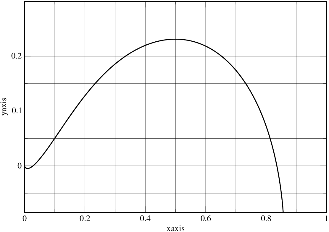
Consider a rate Tanner code ensemble where all VNs have degree and where all CNs are Hamming codes (it was shown in [14, 15] that this ensemble has good spectral shape behavior). The WEF of a Hamming CN is given by , while its local MAP-SSEF and BD-SSEF are given by and respectively. Note that we have in all three cases. A plot of , and obtained by implementation of (18) is depicted in Fig. 1. We observe that satisfies the conditions of Theorem 2. This is reflected by the fact that the weight spectral shape is symmetric with respect to .
Example 2 (Check-hybrid ensemble)
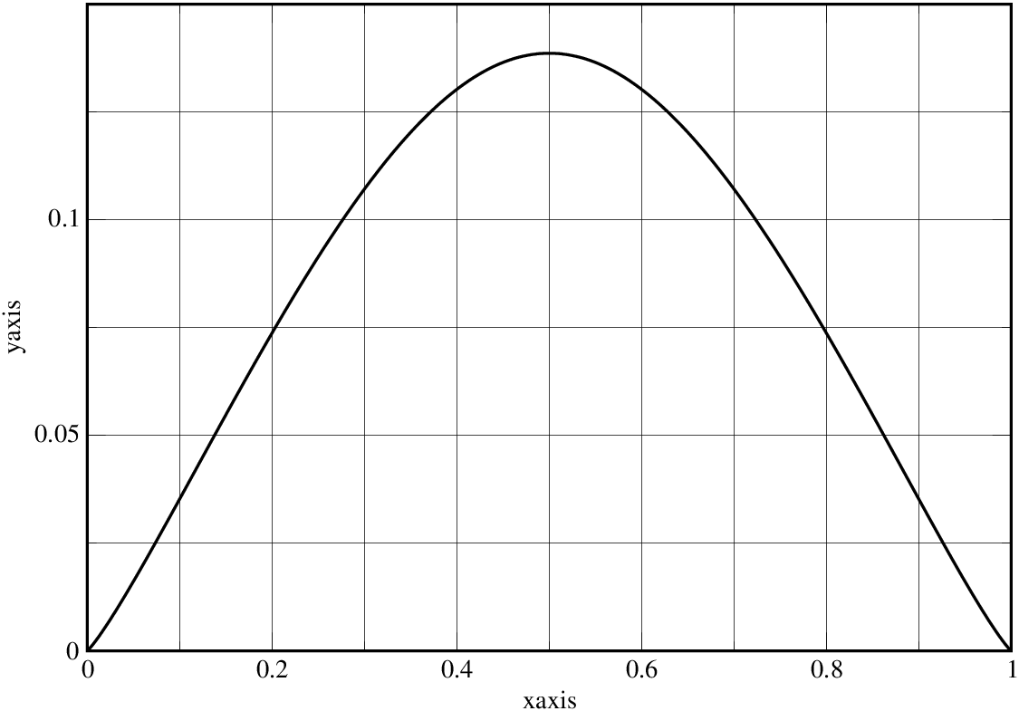
Consider a rate check-hybrid GLDPC code ensemble where all VNs are repetition codes of length and whose CN set is composed of a mixture of two linear block code types (). CNs of type are length- SPC codes with WEF and , while CNs of type are codes with WEF and . The weight spectral shape of this ensemble, obtained from (8), is depicted in Fig. 2. Note that for this ensemble, . This value is not a fixed point of the function defined in (26) (the only fixed point between and is ). As expected, the weight spectral shape does not exhibit any symmetry property.
Example 3 (Ensemble with bad spectral shape behavior)
Consider a rate Tanner code ensemble where all VNs are repetition codes of length and and where all CNs are linear block codes with WEF . This ensemble is known to have bad spectral shape behavior () since we have , where and [12, 13]. A plot of the weight spectrum for this ensemble, obtained from (18) is depicted in Fig. 3. We observe that the plot of is symmetric, due to the fact that is symmetric (). As expected, the derivative of at is positive and hence .
VI Conclusion
A simple expression has been developed for both the weight and the stopping set size spectral shape of GLDPC code ensembles with a regular VN set and a hybrid CN set. Some known results (specifically, an expression for the spectral shape of regular LDPC codes and an asymptotic expression of the spectral shape for GLDPC codes as the normalized weight tends to zero) follow as corollaries of the developed formula. Moreover, symmetry properties of the spectral shape function have been discussed. A sufficient condition and a necessary condition for the weight spectral shape function to be symmetric have been identified.
Appendix A Asymptotic Case
For small , the expression (8) reduces to a known formula first developed in [12] for Tanner codes, and extended in [13] to irregular GLDPC codes. This formula is here obtained as a simple corollary of Theorem 1.
Corollary 2
In the limit where , the growth rate of the weight distribution of a GLDPC code ensemble with a regular VN set fulfills
where denotes the smallest minimum distance of all CN types (i.e. ), denotes the set of CN types with this minimum distance (i.e. ) and denotes Napier’s number.
Proof:
Let . From the definition of given in (7), it is readily shown that if , we must have . Next, note that in (7), each term in the sum on the right-hand side is a rational polynomial in whose denominator tends to unity as , and whose numerator is dominated as by the term corresponding to the lowest power of . Therefore, as , (7) becomes , or equivalently,
| (28) |
Using as , we have that for every as , and so
| (29) |
Appendix B Closed Form Expressions for the Growth Rate
It is worthwhile to note that in some cases, (18) can be expressed in closed form because can be expressed analytically. This is the case, for instance, for the regular LDPC ensemble, for which becomes , where and . This cubic equation in may be solved by Cardano’s method (see, e.g., [17, p. 17]; the discriminant is negative for every , where
The required solution is then uniquely and analytically identified as where and .
Similarly, the weight spectral shape of a regular LDPC ensemble may be expressed in closed form through the solution of a quartic equation.
References
- [1] R. M. Tanner, “A recursive approach to low complexity codes,” IEEE Trans. Inf. Theory, vol. 27, no. 5, pp. 533–547, Sept. 1981.
- [2] R. G. Gallager, Low-density parity-check codes. Cambridge, Massachusetts: M.I.T. Press, 1963.
- [3] G. Liva, W. Ryan, and M. Chiani, “Quasi-cyclic generalized LDPC codes with low error floors,” IEEE Trans. Commun., vol. 56, no. 1, pp. 49–57, Jan. 2008.
- [4] Y. Wang and M. Fossorier, “Doubly generalized LDPC codes,” in Proc. of IEEE 2006 Int. Symp. on Information Theory, Seattle, WA, USA, July 2006, pp. 669–673.
- [5] M. F. Flanagan, E. Paolini, M. Chiani and M. P. C. Fossorier, “Growth rate of the weight distribution of doubly-generalized codes: General case and efficient evaluation,” in Proc. of 2009 IEEE Global Telecommunications Conf., Honolulu, HI, USA, Nov./Dec. 2009.
- [6] S. Abu-Surra, W. E. Ryan and D. Divsalar, “Ensemble enumerators for protograph-based generalized LDPC codes,” in Proc. of 2007 IEEE Global Communications Conf., Washington, DC, USA, Nov. 2007, pp. 1492–1497.
- [7] K. Kasai, C. Poulliat, D. Declercq, T. Shibuya and K. Sakaniwa, “Weight distribution of non-binary LDPC codes,” in Proc. of 2008 Int. Symp. on Inf. Theory and its Applications, Auckland, New Zealand, Dec. 2008, pp. 748–753.
- [8] K. Kasai, T. Awano, D. Declercq, C. Poulliat and K. Sakaniwa, “Weight distributions of multi-edge type LDPC codes,” in Proc. of 2009 IEEE Int. Symp. on Inf. Theory, Seoul, Korea, June/July 2009, pp. 60–64.
- [9] M. Lentmaier, M. B. S. Tavares, and G. P. Fettweis, “Exact erasure channel density evolution for protograph-based generalized LDPC codes,” in Proc. of 2009 IEEE Int. Symp. on Inf. Theory, Seoul, Korea, June/July 2009, pp. 566–570.
- [10] C. -Li Wang, S. Lin and M. P. C. Fossorier, “On asymptotic ensemble weight enumerators of multi-edge type codes,” in Proc. of 2009 IEEE Global Telecommunications Conf., Honolulu, HI, USA, Nov./Dec. 2009.
- [11] C. Di, D. Proietti, I. E. Telatar, T. J. Richardson and R. Urbanke, “Finite-length analysis of low-density parity-check codes on the binary erasure channel,” IEEE Trans. Inf. Theory, vol. 48, no. 6, pp. 1570–1579, June 2002.
- [12] J. -P. Tillich, “The average weight distribution of Tanner code ensembles and a way to modify them to improve their weight distribution,” in Proc. of 2004 IEEE Int. Symp. on Information Theory, Chicago, IL, USA, June/July 2004, pp. 7.
- [13] E. Paolini, M. Chiani and M. Fossorier, “On the growth rate of GLDPC codes weight distribution,” in Proc. of 2008 IEEE Int. Symp. on Spread Spectrum Techniques and Applications, Bologna, Italy, Aug. 2008, pp. 790–794.
- [14] M. Lentmaier and K. Zigangirov, “On generalized low-density parity-check codes based on Hamming component codes,” IEEE Commun. Lett., vol. 3, no. 8, pp. 248–250, Aug. 1999.
- [15] J. J. Boutros, O. Pothier and G. Zémor, “Generalized low density (Tanner) codes,” in Proc. of 1999 IEEE Int. Conf. on Communications, vol. 1, Vancouver, Canada, June 1999, pp. 441–445.
- [16] A. Orlitsky, K. Viswanathan, and J. Zhang, “Stopping set distribution of LDPC code ensembles,” IEEE Trans. Inf. Theory, vol. 51, no. 3, pp. 929–953, Mar. 2005.
- [17] M. Abramowitz and I. A. Stegun, Handbook of mathematical functions with formulas, graphs, and mathematical tables. New York: Dover, 1964.