Extra dimensions in ${\gamma\gamma\to\gamma\gamma}$ process at the CERN-LHC

Central detectors of the Large Hadron Colliders (LHC) experiments ATLAS and CMS at CERN have a pseudorapidity $\eta$ coverage 2.5 for tracking system and 5.0 for calorimetry. In spite of that, a certain amount of particles and momentum flow take place in the very forward directions and are not detected by these detectors. Furthermore, there are contributions to the measured cross sections from elastic scattering and ultraperipheral collisions. For better understanding of the physics from very forward region one needs additional equipments. ATLAS and CMS collaborations developed a program of forward physics with extra detectors located in a region nearly 100m-400m from the interaction point [1]. These are called forward detectors which will be installed very close to the beamline. In connection with these new equipments a research plan has been organized to investigate soft and hard diffraction, high energy photon induced interactions, low-x dynamics with forward jet studies, large rapidity gaps between forward jets, and luminosity monitoring [1, 2, 3]. One of the main features of these forward detectors is to tag the protons with some energy fraction loss $\xi=E_{loss}/E_{beam}$. Based on the ATLAS and CMS working conditions forward detectors will be located in positions from interaction point to have an overall acceptance $0.0015<\xi<0.5$ [4, 5]. Larger $\xi$ is created if the forward detectors are installed closer to the interaction points. Using the forward detectors it is possible to produce high energy photon induced interaction with exclusive two particle final states such as photons or leptons. In this work we are interested in the two photons in the final states. Almost real photons are emitted by each proton and interact each other to provide two photons $\gamma\gamma\to\gamma\gamma$. Forward detectors will detect the energy loss of the deflected protons but the central detector will identify the final photons with rapidity $|\eta|<2.5$ and $p_{T}>(10-20)$ GeV. Emitted photons by the protons with small angles have a spectrum depending on virtuality $Q^{2}$ and energy $E_{\gamma}$. This is described by the equivalent photon approximation [6, 7]. The spectrum differs from the pointlike electron positron case by taking into account the electromagnetic form factors

where

Here E is the energy of the proton beam which is related to the photon energy by $E_{\gamma}=\xi E$ and $m_{p}$ is the mass of the proton. The magnetic moment of the proton is $\mu^{2}_{p}=7.78$, $F_{E}$ and $F_{M}$ are functions of the electric and magnetic form factors. The integration of the cross section $d\sigma_{\gamma\gamma\to\gamma\gamma}$ should be made over the photon spectrum

where the effective photon luminosity $dL^{\gamma\gamma}/dW$ is given by

with

Here W is the invariant mass of the two photon system $W=2E\sqrt{\xi_{1}\xi_{2}}$ and maximum virtuality is $Q^{2}_{max}=2$ $\mbox{GeV}^{2}$. In Fig.1 effective $\gamma\gamma$ luminosity is shown as a function of the invariant mass of the two photon system where pp energy $\sqrt{s}=14$ TeV is taken.

It is interesting to search for new physics with invariant two photon mass $W>1$ TeV by the photon-induced two photon final states with available luminosity. In this work, we explore the phenomenology of extra dimensions in the framework of the Arkani-Hamed, Dimopoulos and Dvali(ADD) model of large extra dimensions and Randall-Sundrum (RS) model of warped extra dimensions via the photon induced process $pp\to p\gamma\gamma p$ at the LHC. We also summarize the Standard Model ${\gamma\gamma\to\gamma\gamma}$ loop process in its own right and as a background. $\sqrt{s}=14$ TeV is considered when the proton-proton center of mass energy is needed.

In this section, we review the properties of the helicity amplitudes of the one-loop ${\gamma\gamma\to\gamma\gamma}$ process and provide the SM cross sections at LHC using the steps taken in the previous section. An experiment involving $\gamma\gamma$ scattering at high energies has not been done yet. In this respect, the precise determination of this cross section have a special importance to test the renormalization procedure of the parts of the SM containing W gauge bosons. Furthermore, this loop process becomes a background for new physics searches through $\gamma\gamma$ scattering.

One-loop diagrams involve charged fermions and W bosons. For the $\sqrt{s_{\gamma\gamma}}>200-250$ GeV W boson contribution is dominant over the lepton and quark contributions [8]. This nice property allows to separate the contributions of the fermions and W bosons in the cross section. There are sixteen helicity amplitudes contributing to the process. Fermion contribution with mass $m_{f}$ and charge $Q_{f}$ to the helicity amplitudes can be given simply by neglecting the terms like $m_{f}^{2}/\hat{s}$, $m_{f}^{2}/\hat{t}$ and $m_{f}^{2}/\hat{u}$

where invariant Mandelstam variables are defined as $\hat{s}=(p_{1}+p_{2})^{2}$, $\hat{t}=(p_{1}-p_{3})^{2}$ and $\hat{u}=(p_{2}-p_{3})^{2}$. The remaining amplitudes can be related to those given by the equations above by parity and Bose symmetry.

It is possible to get simple expressions for W contribution when the terms like $m_{W}^{2}/\hat{s}$, $m_{W}^{2}/\hat{t}$ and $m_{W}^{2}/\hat{u}$ are neglected

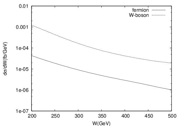
In the W contribution, one should note that the dominant terms arise from the imaginary part of the helicity amplitude for the energy region satisfying the approximation $m_{W}^{2}<<\hat{s}$. For $m_{W}^{2}>>\hat{s}$ contribution of W boson decreases and fermion contribution drastically increases and much larger than the W contribution. The top quark contribution is neglected above because it is much lower than the light quark and W contribution in both regions . Fig.2 shows the contributions of fermions and W boson to the cross sections $pp\to p\gamma\gamma p$ as a function of invariant mass of the two photon system for the energy region of 200-500 GeV and for the rapidity $|\eta|<2.5$. Dominance of the W contribution is clear in this energy region. The total cross section of fermion contributions for W=20-80 GeV, $|\eta|<2.5$ is 0.723 fb and W boson contribution for W=200-500 GeV, $\sqrt{|\hat{t}|}>200$ GeV, $\sqrt{|\hat{u}|}>200$ GeV, $|\eta|<2.5$ is 0.074 fb. In both cases we take into account $0.0015<\xi<0.5$. Rapidity distributions of W-boson and fermion contributions to the cross section are provided in Fig.3 for two energy scales of two photon system 20-80 GeV and 200-500 GeV. As it is seen, the curves which belong to the fermions and W boson have different behaviour as rapidity changes.

ATLAS detector at the LHC is capable of detecting of photons efficiently(up to 90%) based on its wide range of parameters [9]. If sufficient luminosity of 100-200 $fb^{-1}$ is available at LHC, the cross sections of the contributions of W boson and fermions can be observable separately in the $\gamma\gamma\to\gamma\gamma$ one-loop SM process. All the cross sections and related distributions in this paper are given in the laboratory system i.e. center of mass system of the two incoming protons.

The Hierarchy problem in particle physics arises from the fact that there is a large difference in energy between the electroweak scale which is a few hundreds of GeV and gravity scale that is the Planck scale $M_{Pl}\sim 10^{19}$GeV in a four dimensional spacetime. Extra space dimensions higher than three are already known in string theory. Following the string theory ideas, three space dimensional world is called a ”wall” or 3-brane where all Standard Model particles are confined to this wall. The D-dimensional spacetime, $D=3+\delta+1$, with $\delta$ extra space dimensions is called ”bulk” where 3-brane is embedded in it. The methods how to handle hierarchy problem are model dependent.

In the model proposed by Arkani-Hamed, Dimopoulos and Dvali gravity propagates in the bulk but SM fields can not go out of the 3-brane [10]. The solutions of the linearized equations of motion of the metric field are the Kaluza-Klein tower in D dimensions. Upon integrations over extra dimensions, the final 4-dimensional fields are the Kaluza-Klein modes. Zero mode of the KK field is massless that leads to the graviton in 4-dimensions. Excited modes of the KK fields become massive. According to this model extra dimensions are compactified with a compactification radius $r_{c}\sim$mm-fermi (or $1/r_{c}\sim$eV-MeV) by which the KK mode spacing is specified. This mode spacing is very small with respect to the typical collider energies. This property allows for the summation over large number of KK states. ADD model is also known as the large extra dimension model due to large compactification radius. Strong gravity occurs in $D=4+\delta$ dimensions because of the overall effect of the KK states. Thus its effective interactions in 4-dimensions with the Standard Model particles are expected to be measurable at collider energies. The relation between the Planck Mass $M_{Pl}$ and the corresponding scale $M_{D}$ in D-dimensions can be written by the use of the compactified volume $V_{\delta}$

When $M_{D}$ is assumed to be in TeV region, large higher dimensional volume of $V_{\delta}$ makes $M_{Pl}$ large with $\delta=2-7$. This result implies that Planck scale $M_{Pl}$ is not the fundamental scale afterall. The large gap between the electroweak and Planck scale is compensated by the large compactification scale of the extra dimensions. It should be pointed out that this does not resolve the hierarchy problem but large gap shifts to the compactification radius and the inverse of the electroweak scale.

There are three Feynman diagrams containing KK propagators in s, t and u channels. Let us now calculate the Feynman amplitudes for the subprocess $\gamma\gamma\to\gamma\gamma$ for three channels using the KK-$\gamma\gamma$ vertex function $\Gamma^{\alpha\beta\rho\sigma}$ [11]

where $p_{1},p_{2}$, $p_{3},p_{4}$ are incoming and outgoing photon momenta. The coupling constant $\kappa$ is related to the Newton constant $G^{(4+\delta)}_{N}$ in $D=4+\delta$ dimension by $\kappa^{2}=16\pi G^{(4+\delta)}_{N}$. Explicit forms of the tensors $C^{\alpha\beta\rho\sigma}$ and $D^{\alpha\beta\rho\sigma}$ are given by

where $\eta^{\rho\sigma}$ is the metric tensor of the flat space in four dimensions. The square of the amplitudes are

Lorentz invariant Mandelstam variables $\hat{s}$, $\hat{t}$ and $\hat{u}$ are given in previous section. Here the factor due to initial spin average and statistical factor from identical final photons are absent. From previous sections we know that only W boson contributes to the Standard Model one-loop amplitudes for the energies $\sqrt{\hat{s}}>200$ GeV. At these energies the dominant terms are imaginary. This makes the interference terms with the SM negligible based on the fact that KK contributions to the amplitudes are real.

KK propagator $D(\hat{s})$ contains summation over Kaluza-Klein modes which can be calculated without specifying any specific process. Since the KK tower is an infinite sum, ultraviolet divergences are present in tree level process. Thus we need a cutoff procedure. For the purpose of phenomenological applications basic steps of the approach followed by Han et al. [11] are given below

The last equality is obtained by approximating the infinite KK sum by an integral. The real part in square bracket in the right hand side comes from the narrow resonant states of single KK mode. $I(x)$ is related to nonresonant summation of infinite KK tower where $x=\frac{\Lambda_{c}}{\sqrt{\hat{s}}}$ and $\Lambda_{c}$ is defined as the ultraviolet cutoff energy. The definition of $\kappa^{2}=16\pi/M_{Pl}^{2}$ and Eq.(3.1) have been used to reach the form on the right side. The explicit form of $I(x)$ is written for even and odd values of $\delta$

The relation between the unknown cutoff energy $\Lambda_{c}$ and the fundamental scale $M_{D}$ is not clear unless the full theory is known. The connection $\Lambda_{c}<M_{D}$ can be given on the ground of the string theory. In several calculations in the literature the equality $M_{D}\simeq\Lambda_{c}$ demonstrates the lower limit of the fundamental scale $M_{D}$. Within this work $M_{D}\simeq\Lambda_{c}$ is set for KK graviton propagator of ADD model. $\kappa^{2}D(\hat{s})$ is dominated by nonresonant ultraviolet contribution for $x>>1$. Then approximate result can be obtained for comparison with other notations in the literature [11].

This corresponds to the result of Giudice et al. [11] $\Lambda_{c}=\Lambda_{T}$ for $\delta=4$. The same form can be used for t and u channels.

Collider signals of virtual graviton exchange manifest itself as the deviations from the SM in the cross section. Furthermore, the angular distributions of the final particles are dedicated to spin-2 nature of the graviton. First we show the rapidity distribution of the final photons in Fig.4 for the contribution of the KK graviton with $M_{D}=1500$ GeV to the total cross section of the main process $pp\to p\gamma\gamma p$ in the photon induced interactions at LHC with forward detectors. We consider two acceptance regions of the forward detectors $0.0015<\xi<0.5$ and $0.1<\xi<0.5$. Each curve correspons to a rapidity cut $|\eta|<2$ with additional cuts on variables $\sqrt{\hat{s}}>200$ GeV, $\sqrt{|\hat{t}|}>200$ GeV and $\sqrt{|\hat{u}|}>200$ GeV. Requirement both $\sqrt{|\hat{t}|}>200$ and $\sqrt{|\hat{u}|}>200$ GeV induces a cut $|\eta|<2$. We did not include SM one-loop contribution on the ground of its smallness that can be seen in Fig.3. All cuts are also given in the laboratory frame of the protons as stated earlier

$p_{T}$ distribution of the final photons for the KK terms of the cross section is plotted in Fig.5 with $|\eta|<2$ and two acceptance regions $0.0015<\xi<0.5$ and $0.1<\xi<0.5$. In Fig.4 and Fig.5 both curves for different acceptance regions seem almost identical in shape and in the magnitude. This leads to the fact that the cuts on $\sqrt{|\hat{t}|}$ and $\sqrt{|\hat{u}|}$ are satisfied by high $\sqrt{\hat{s}}$ values. It is clear that the contribution of the energy from the region $0.0015<\xi<0.1$ to the cross section of the KK terms is negligible for the cuts given above. Thus, it is more convenient to use the region $0.1<\xi<0.5$ for the rest of our calculations. In this energy region cross section from SM one-loop contributions is the order of $10^{-4}$fb where we ignore it from here on.

Next, we calculate 95% C.L. bounds on the $M_{D}$ as a function of the integrated LHC luminosity for the acceptance region $0.1<\xi<0.5$ with the above restrictions on the rapidity and the Mandelstam variables. Poisson distributed events are considered for statistical analysis. The estimations are shown in Fig.6 where the acceptance region $0.1<\xi<0.5$ is good enough to feel the KK graviton exchange in the process $pp\to p\gamma\gamma p$ via two photon fusion.

Randall and Sundrum proposed a model to handle the large hierarchy between the electroweak and the gravity scales. In this model curvature in higher dimensions play the important role to remove this large hierarchy. The metric in 5D is a solution to Einstein’s equations respecting the 4D Poincare invariance [12]

where y is the $5^{th}$ dimension which is parametrized as $y=r_{c}|\Phi|$ with $r_{c}$ being the compactification radius of the extra dimension. Angular coordinate $\Phi$ has the limits of $0\leq|\Phi|\leq\pi$. First term in this metric is the Minkowski spacetime metric in 4D multiplied by an exponential factor which is called warp factor containing fifth dimension and the degree of the curvature k. This model includes two 3-brane with opposite and equal tensions at the boundaries of a 5D Anti-de-Sitter space. Each boundary has 4D Minkowski metric and y is orthogonal to each 3-brane. The distance between the two walls is $y=\pi r_{c}$. The wall at $y=0$ on which Gravity is localized is called Planck brane. The other wall at $y=\pi r_{c}$ is referred to TeV brane where SM fields live on. Gravity propagates in $5^{th}$ dimension.

Starting with 5D action, the 4D effective lagrangian containing the interaction of the KK gravitons with the matter fields can be obtained by

where $T^{\alpha\beta}(x)$ is the energy momentum tensor of the matter field in the Minkowski space and $\bar{M}_{Pl}=M_{Pl}/\sqrt{8\pi}$ is the reduced Planck scale. $h^{(n)}_{\alpha\beta}(x)$ describes the KK modes of the graviton on the 3-brane. The masless zero KK mode decouples from the sum and its coupling strength is $1/\bar{M}_{Pl}$. The massive KK states has the coupling of $(1/\Lambda_{\pi})\sim 1/\mbox{TeV}$ with $\Lambda_{\pi}=e^{-kr_{c}\pi}\bar{M}_{Pl}$.

The relation between 5D fundamental Planck scale M and usual 4D reduced Planck scale is

Taking $k\sim M_{Pl}$ we reach the relation $M\sim M_{Pl}$. Therefore, there is no additional hierarchy created by the model. If $kr_{c}$ has the value $\sim 10-12$ all the physical processes take place in TeV scale on TeV-brane. This demonstrates the fact that the hierarchy is generated by the warp factor.

The mass spectrum created by KK modes of the graviton in the RS model is given by [12]

where $x_{n}$ are the roots of the Bessel function of order 1 $J_{1}(x_{n})=0$. The first values are $x_{1}=3.83$, $x_{2}=7.02$ and $x_{3}=10.17$. The scale of the masses is $m_{n}\sim\Lambda_{\pi}\sim\mbox{TeV}$ on the ground of $\beta\sim 1$. It is clear that the each excitation should be sizable separately at colliders. The appropriate parameters to describe the RS scenario for phenomenological applications are $\Lambda_{\pi}$ and $\beta$. The only graviton propagator differs from the ADD case in the squared amplitude for $\gamma\gamma\to\gamma\gamma$

with $\rho=1$ is used in the width $\Gamma_{n}$ of the individual KK graviton. Limits on the parameter $\beta$ can be found for the first graviton mode with mass $m_{1}$. The estimation for 95% C.L. parameter exclusion region is shown in Fig.7 for the integrated LHC luminosities; $50fb^{-1}$, $100fb^{-1}$ and $200fb^{-1}$, with the acceptance region $0.1<\xi<0.5$.

In the approximation $m^{2}_{n}>>\hat{s}$, $m^{2}_{n}>>\hat{t}$, $m^{2}_{n}>>\hat{u}$ KK graviton propagators for three channels take the form

Fig.8 shows 95% C.L. search reaches in the $\Lambda_{\pi}-\beta$ plane for an acceptance region of $0.1<\xi<0.5$ and LHC luminosities given before.

Photon-photon collision at LHC with diphoton invariant mass $W>1$ TeV allows to study physics at TeV scale beyond the SM with a sufficient luminosity. There is no existing collider with this property except the LHC itself. It is worth mentioning that two photon final state is one of the cleanest channel to search for any deviation from the SM physics. For this reason, we have investigated how the photon-induced two photon final state can extend the bounds on the model parameters of extra dimensions in the framework of the ADD and RS models. Taking an acceptance region of $0.1<\xi<0.5$ we have obtained constraints on the fundamental scale $M_{D}$ in the ADD model for a LHC luminosity interval 1-200 $fb^{-1}$. Exclusion regions of the parameter pairs of RS model $\beta-m_{1}$ and $\Lambda_{\pi}-\beta$ have been provided for the LHC luminosities $50fb^{-1}$, $100fb^{-1}$ and $200fb^{-1}$. Possible background coming from the SM one-loop diagrams can be neglected in the energy and rapidity range defined above sections. Excluded area of the model parameters that we have found from the process $pp\to p\gamma\gamma p$ extends to wider regions than the case of the colliders LEP and Tevatron [13, 14]. Certainly, the challenging processes are the quark antiquark annihilation into two photons $q\bar{q}\to\gamma\gamma$ as well as gluon fusion $gg\to\gamma\gamma$ with KK graviton exchange at the LHC itself [14]. Although $\gamma\gamma\to\gamma\gamma$ process has cleaner enviroment, $gg,q\bar{q}\to\gamma\gamma$ process needs a sophisticated background analysis. The excluded regions of this paper are wider than the case of the similar study using the subprocess $\gamma\gamma\to\ell^{+}\ell^{-}$ at LHC [15].

References

- [1] C. Royon, Mod. Phys. Lett. A 18,2169 (2003); M. Boonekamp, R. Peschanski and C. Royon, Phys. Rev. Lett. 87 251806 (2001); Nucl. Phys. B669, 277 (2003); M. Boonekamp, A. De Roeck, R. Peschanski and C. Royon, Phys. Lett. B550, 93 (2002); V.A. Khoze, A.D. Martin and M.G. Ryskin, Eur. Phys. J. C 19, 477 (2001); 24, 581 (2002); 55, 363 (2008); Phys. Lett. B650, 41, (2007); A.B. Kaidalov, V.A. Khoze, A.D. Martin and M.G. Ryskin, Eur. Phys. J. C33, 261 (2004); 31, 387 (2003); O. Kepka and C. Royon, Phys. Rev. D78, 073005 (2008).
- [2] V.A. Khoze, A.D. Martin and M.G. Ryskin, Eur. Phys. J. C23, 311 (2002).
- [3] N. Schul and K. piotrzkowski, Nucl. Phys. Proc. Suppl., 179-180, 289-297 (2008); arXiv:0806.1097.
- [4] C. Royon(RP220 Collaboration), arXiv:0706.1796.
- [5] M.G. Albrow et al. (FP420 R and D Collaboration), arXiv:0806.0302.
- [6] V.M. Budnev, I.F. Ginzburg, G.V. Meledin and V.G. Serbo, Phys. Rep. 15, 181 (1975).
- [7] G. Baur, K. Hencken, D. Trautmann, S. Sadowsky and Y. Kharlov, Phys. Rep. 364, 359 (2002); K. Piotrzkowski, Phys. Rev. D 63(2001) 071502.
- [8] G. Jikia and A. Tkabladze, Phys. Lett. B 323, 453 (1994); G.J. Gounaris, P.I. Porfyriadis and F.M. Renard, Phys. Lett.B 452, 76 (1999); G.J. Gounaris, P.I. Porfyriadis and F.M. Renard, Eur. Phys. J.C9,673 (1999).
- [9] ATLAS LIQUID ARGON CALORIMETER collaboration, J. Colas et al., Nucl. Instrum. Meth. A550,96 (2005); ATLAS collaboration, M.D. Baker, ATL-PHYS-PROC-2009-059 [arXiv:0907.4158]
- [10] N. Arkani-Hamed, S. Dimopoulos and G. Dvali, Phys. Lett. B 429, 263 (1998); Phys. Rev. D 59, 086004 (1999); I. Antoniadis, N. Arkani-Hamed, S. Dimopoulos and G. Dvali, Phys. Lett. B 436, 257 (1998).
- [11] G.F. Guidice, R. Ratazzi and J.D. Wells, Nucl. Phys. B544, 3 (1999); E.A. Mirabelli, M. Perelstein and M.E. Peskin, Phys. Rev. Lett. 82, 2236 (1999); T. Han, J.D. Lykken and R.-J. Zhank, Phys. Rev. D 59 105006 (1999); J.L. Hewett, Phys. Rev. Lett. 82, 4765 (1999).
- [12] L. Randall and R. Sundrum, Phys. Rev. Lett. 83, 3370 (1999); W.D. Goldberger and M.B. Wise, Phys. Rev. Lett. 83, 4922 (1999).
- [13] H. Davoudiasl, J.L. Hewett and T.G. Rizzo, Phys. Rev. Lett. 84, 2080 (2000); V.M. Abazov et al. D0 Collaboration, Phys. Rev. Lett. 95, 091801 (2005); E.W. Dvergsnes, P. Osland, A.A. Pankov and N. Paver, Phys. Rev. D 69(2004) 115001; P. Osland, A.A. Pankov, A.V. Tsytrinov and N. Paver, arXiv:0902.1593(hep-ph).
- [14] O.J.P. Eboli, T. Han, M.B. Magro and P.G. Mercadante, Phys. Rev. D 61, 094007 (2000).
- [15] S. Atag, S.C. Inan and I. Sahin, Phys. Rev. D 80, 075009 (2009)