Sommerfeld Enhancements for Thermal Relic Dark Matter

Given values of $m_{X}$, $m_{\phi}$, and $\alpha_{X}$, we must determine the relic density $\Omega_{X}$. The formalism of thermal freeze out is well developed [31, 32]. Here we review this formalism in sufficient generality to accommodate novel effects resulting from Sommerfeld enhancements.

The evolution of the abundance of a thermal relic $X$ is governed by the Boltzmann equation

where $n_{X}$ is the number density of the dark matter particles, $n_{X}^{\text{eq}}$ is its value in equilibrium, $H$ is the Hubble constant, and $\langle\sigma_{\text{an}}v_{\text{rel}}\rangle$ is the annihilation cross section multiplied by the relative velocity, averaged over the dark matter velocity distribution. Changing variables from $t\to x=m_{X}/T$ and $n_{X}\to Y=n_{X}/s$, where $s$ is the entropy density, the Boltzmann equation becomes

where $m_{\text{Pl}}=G_{N}^{-1/2}\simeq 1.2\times 10^{19}~\text{GeV}$ is the Planck mass, and $g_{*s}$ and $g_{*}$ are the effective relativistic degrees of freedom for entropy and energy density, respectively. In this section we will assume that the particles $X$ annihilates to are in thermal equilibrium at the time of freeze out. We will revisit this issue in Sec. III.2, where we show that this requirement leads to significant constraints if the dominant annihilation is to the dark force carriers.

To evaluate the relic density, we first evolve it to the time of chemical decoupling, when the annihilation rate $\Gamma_{\text{an}}\equiv n_{X}\langle\sigma_{\text{an}}v_{\text{rel}}\rangle$ is approximately the expansion rate $H$. As discussed in Sec. II, we assume the annihilation cross section has the form $\sigma_{\text{an}}v_{\text{rel}}=(\sigma_{\text{an}}v_{\text{rel}})_{0}S$, where $(\sigma_{\text{an}}v_{\text{rel}})_{0}$ is the $S$-wave, tree-level cross section, and $S$ is the Sommerfeld enhancement. Up to the time of freeze out, the Sommerfeld effect is insignificant, and so the standard results for $S$-wave annihilators apply: defining freeze out by

where $c$ is a constant, freeze out occurs at

where $g$ is the number of degrees of freedom of the dark matter particle; we take $g=2$. To match numerical results, $c\sim 1$; we choose $c=1$ and have checked that varying $c$ from 1/2 to 2 has no appreciable effect. To further test this approximation we have also numerically evolved Eq. (10) from $x=20$ to $x=100$ (when the equilibrium abundance is effectively zero) and then used Eq. (12) to evolve into the late Universe. This numerical calculation typically results in 10% smaller relic abundance. Given the excellent agreement, we set $c=1$ and with this choice, Eqs. (11) and (12) determine $Y(x_{f})$, the abundance at freeze out.

After freeze out, $Y^{\text{eq}}$ quickly becomes insignificant. Neglecting it, we may solve Eq. (10) to find

where $x_{\text{kd}}$ is the value of $x$ at kinetic decoupling and $x_{\text{s}}$ is its value when annihilations become insignificant and we may stop the integration. We have broken the integral into two to emphasize that there are two eras: before and after the temperature of kinetic decoupling $T_{\text{kd}}$. Before $T_{\text{kd}}$, the dark matter’s velocity distribution is thermal with temperature $T_{X}=T$. After $T_{\text{kd}}$, the dark matter’s velocity distribution initially remains thermal, but $T_{X}$ drops as $a^{-2}$, while $T$ drops as $a^{-1}$, where $a$ is the scale factor, and so $T_{X}=T^{2}/T_{\text{kd}}$. Eventually, the dark matter’s velocity distribution need not even be thermal. We discuss the value of $T_{\text{kd}}$ and the issue of non-thermal velocity distributions in Secs. III.3 and III.4, respectively.

When the dark matter distribution is thermal with temperature $T_{X}$, the thermally-averaged cross section in the non-relativistic limit is

where $f(\vec{v})$ is the dark matter’s velocity distribution, $v_{\text{rel}}=|\vec{v}_{1}-\vec{v}_{2}|$, and

the most probable velocity. For the Sommerfeld-enhanced annihilation cross section, this becomes

where

is the Sommerfeld enhancement averaged over a thermal distribution with temperature $T_{X}=m_{X}/x_{X}$.

In the relic density calculation, we have implicitly assumed that, when the $X$ particles chemically decouple, the force carriers $\phi$ are in thermal equilibrium with the massless particles of the standard model. The force carriers are expected to interact with the standard model, as their decays to standard model particles typically provide the indirect signals. In a simple example, if $\phi$ is a U(1) gauge boson, it may mix with the standard model photon through kinetic mixing terms $\sim\epsilon F_{\mu\nu}^{\text{EM}}F^{\phi\,\mu\nu}$. After diagonalizing the $\phi$-photon system, standard model particles with charge $Q$ have hidden charge $\epsilon Q$ [33], and so the $\phi$ particles decay through $\phi\to f\bar{f}$, where $f=e,\mu,u,d,s,\ldots$. The largest kinetic mixing parameter allowed by current particle physics constraints is $\epsilon\sim 10^{-3}$ [34, 35].

The existence of $\phi$ interactions with the visible sector does not, however, guarantee that they are efficient enough to bring the $\phi$ particles in thermal equilibrium. Here we determine sufficient conditions for the kinetic mixing example to guarantee the equilibration of $\phi$ particles. The leading $\phi$ number-changing interactions between the $\phi$ particles and the visible sector are decays $\phi\to f\bar{f}$ and inverse decays $f\bar{f}\to\phi$. Other $\phi$ number-changing processes, such as $f\bar{f}\to\phi\gamma$, $q\bar{q}\to\phi g$, and $f\gamma\to f\phi$, are parametrically suppressed compared to these and subdominant. For temperatures $T\gg m_{\phi}$, the decay and inverse decay processes balance (since $f,\bar{f}$ are in chemical equilibrium), and we may simply compare the decay rate to the expansion rate  [36].

For $T\gg m_{\phi}$, the thermally-averaged decay rate for $\phi\to f\bar{f}$ in the lab frame is $\langle\Gamma_{\phi}\rangle\simeq(\epsilon^{2}/3)\sum_{f}(Q_{f}^{2}N^{f}_{c})\alpha_{\text{EM}}m_{\phi}(m_{\phi}/T)$, where we have averaged over three $\phi$ polarizations, $Q_{f}$ and $N^{f}_{c}$ are the standard model charge and number of colors for fermion $f$, the sum is over all fermions with mass $m_{f}<m_{\phi}/2$, and the last factor of $m_{\phi}/T$ is from time dilation. Note that the decay process is inefficient at early times and high temperatures, but as $T$ drops, $\langle\Gamma_{\phi}\rangle$ increases and $H$ decreases, and so the $\phi$ particles may come into thermal equilibrium with the the standard model. The expansion rate is $H\simeq 1.66\,g_{*}^{1/2}T^{2}/m_{\text{Pl}}$; at freezeout, $g_{*}\simeq 100$. Requiring $\langle\Gamma_{\phi}\rangle\gtrsim H$ at $T_{f}\simeq m_{X}/25$ yields $\epsilon\gtrsim 3\times 10^{-6}$ for $m_{\phi}=\text{GeV}$ and $m_{X}=\text{TeV}$.

If the above constraint is not satisfied, then the hidden sector may be at a different temperature from the standard model, modifying the dark matter freezeout. Such scenarios have been considered in Ref. [37], and the difference in temperatures has a significant impact on the dark matter relic density. These considerations may be important for some models, but here we assume that Eq. (18) is satisfied and $m_{\phi}\ll T_{f}\simeq m_{X}/25$, so that the $\phi$ particles are in thermal contact with the standard model at freeze out and their number density is close to the thermal prediction.

We note here that the calculation above does not guarantee chemical equilibrium. For the $\phi$ particles to produce $X$ through $\phi\phi\rightarrow XX$, we need the tail of the $\phi$ distribution to be populated thermally. To check this, we approximate the decay rate for $\phi$ with energies of order $m_{X}$ as $(\epsilon^{2}/3)\sum_{f}(Q_{f}^{2}N^{f}_{c})\alpha_{\text{EM}}m_{\phi}(m_{\phi}/m_{X})$. If this decay rate is larger than the expansion rate, then the inverse process will also be in equilibrium and hence thermally populate the tail of the $\phi$ distribution. Comparing this to the expansion rate at $T_{f}\simeq m_{X}/25$ we obtain that

In setting the bound above, we have not considered scattering interactions with standard model fermions (and the resulting changes in kinetic energy for $\phi$) because these processes are proportional to $\epsilon^{4}$ and hence considerably slower that the inverse decay process.

To summarize, for the $\phi$ particles to be in thermal equilibrium with the standard model at freezeout requires that Eq. (18) is satisfied and $m_{\phi}\ll T_{f}\simeq m_{X}/25$. We will assume these conditions hold in our analysis, but we note that they do not necessarily hold. In particular, if $m_{\phi}\sim T_{f}$, the number of $\phi$ particles at freezeout is reduced, which reduces the $X$ relic density, strengthening the bounds on $S_{\text{eff}}$ we determine below.

After freeze out, dark matter particles remain kinematically coupled to the thermal bath through elastic scattering. Kinetic decoupling occurs later, when the momentum transfer rate drops below the Hubble expansion rate. We define the kinetic decoupling temperature $T_{\text{kd}}$ by $\Gamma_{k}(T_{\text{kd}})=H(T_{\text{kd}})$, where $\Gamma_{k}$ is the momentum transfer rate. It may be approximated as

where $n_{r}$ is the number density of the relativistic species in the thermal bath, and $\langle\sigma_{\text{el}}v_{\text{rel}}\rangle$ is the thermally-averaged cross section for elastic scattering between dark matter particles and the relativistic particles in the thermal bath.

We first consider the model-independent elastic scattering off the hidden sector thermal bath of $\phi$ particles [38]. For $T\lesssim m_{\phi}$, $n_{\phi}$ is Boltzmann suppressed, and so this process will not be able to maintain kinetic equilibrium. For $T\gtrsim m_{\phi}$, the thermally-averaged $X\phi\to X\phi$ cross section is

the Thomson scattering cross section. Given the $\phi$ number density $n_{\phi}\sim T^{3}$, the momentum transfer rate is $\Gamma_{k}\sim\alpha_{X}^{2}T^{4}/m_{X}^{3}$, and this is equal to $H\sim T^{2}/m_{\text{Pl}}$ at

where we have normalized the expression to typical parameters that give the correct relic density in the presence of Sommerfeld enhancement. Halo shape constraints require $m_{\phi}\gtrsim 30~\text{MeV}$ [2], and so for all physically viable and relevant parameters,

This is the temperature of kinetic decoupling from the hidden thermal bath. It is quite model-independent, as it assumes only the $X$-$\phi$ interactions required in all Sommerfeld enhancement scenarios, and so it provides a maximal value of $T_{\text{kd}}$ in Sommerfeld scenarios.

Dark matter particles may also be kept in kinetic equilibrium through scattering off the visible sector’s thermal bath. This is more model dependent, but as discussed in Sec. III.2, if $\phi$ is a U(1) gauge boson, it may mix with the standard model photon. After diagonalizing the $\phi$-photon system, standard model particles with charge $Q$ have hidden charge $\epsilon Q$, inducing new energy transfer processes. The most efficient process is $Xe\to Xe$ scattering through $t$-channel $\phi$ exchange. For $T\lesssim m_{e}$, Boltzmann suppression of the electron number density makes the interaction inefficient. At temperatures $m_{\phi}\gtrsim T\gtrsim m_{e}$, the corresponding cross section is [39]

The momentum transfer rate $\Gamma_{k}\sim\epsilon^{2}\alpha_{\text{EM}}\alpha_{X}T^{6}/(m_{\phi}^{4}m_{X})$ is equal to the expansion rate at temperature

and so the resulting temperature of kinetic decoupling from the visible sector’s thermal bath is

where we have again normalized $\alpha_{X}$ and $m_{X}$ to typical freeze out parameters, and additionally normalized $m_{\phi}$ to its smallest possible value and $\epsilon$ to its largest allowed value. When $\epsilon$ is near its maximal value, $T_{\text{kd}}^{e}(\epsilon)<T_{\text{kd}}^{\phi}$, and so interactions with the visible thermal bath delay kinetic decoupling. We denote the lowest possible kinetic decoupling temperature

and will explore the dependence of our results on the temperature of kinetic decoupling by varying it between its maximal value $T_{\text{kd}}^{\phi}$ and its minimal value $T_{\text{kd}}^{e}$.

By crossing symmetry, the visible sector scattering interaction also implies an annihilation process $XX\to e^{+}e^{-}$. In principle, this also enters the thermal relic density calculation. The cross section is $\langle\sigma_{\text{an}}v_{\text{rel}}\rangle\sim\epsilon^{2}\alpha_{\text{EM}}\alpha_{X}/m_{X}^{2}$, however, and the $\epsilon^{2}$ suppression makes this subdominant for all relevant cases.

Before kinetic decoupling, dark matter particles have the same temperature as the thermal bath and a Maxwell-Boltzmann phase space distribution. Usually one assumes that the phase space distribution remains Maxwell-Boltzmann after kinetic decoupling. However, this is not necessarily true in scenarios with Sommerfeld-enhanced annihilation, because slow particles annihilate with larger cross sections. This preferentially depletes the low velocity population and may distort the phase space distribution. In this case, the standard formulae used to compute the relic density of dark matter are not valid and one needs to explicitly consider the effect of annihilations using the full phase space distribution.

As discussed in Refs. [40, 39, 2, 41, 42], however, the $\phi$ field mediates self-scattering between dark matter particles. If the self-scattering rate is higher than the Hubble expansion rate, the momentum exchanged in these self-interactions with be sufficient to maintain thermal equilibrium. The momentum transfer of particles interacting through Yukawa potentials has been studied in Refs. [43, 44]. Although the authors of these studies were interested in slow and highly charged particles moving in plasmas with screened Coulomb potentials, they approximated these potentials by Yukawa potentials, and so their results are exactly applicable in the current particle physics context. The numerical results of these studies for the momentum transfer cross section are accurately reproduced by [43, 44]

where $\beta=2\alpha_{X}m_{\phi}/(m_{X}v_{\text{rel}}^{2})$.

Given these results, we may calculate the dark matter self-scattering rate and compare it to the Hubble expansion rate. The self-scattering rate is given by [2]

where $n_{X}$ is the dark matter density. This sets the time scale to change velocities by ${\cal O}(1)$. To find the rate to change the kinetic energy by ${\cal O}(1)$, one would divide the above rate by a factor of 3. However, such details are not important for the present calculation. $H$ and $\Gamma_{s}$ are presented in Fig. 2 for two representative cases.

We may define the self-scattering decoupling temperature $T_{\text{nt}}$ by $\Gamma_{s}(T_{\text{nt}})=H(T_{\text{nt}})$; after $T_{\text{nt}}$, the dark matter velocity distribution may become non-thermal. To derive an approximate expression for $T_{\text{nt}}$, note that to have the right relic abundance, the co-moving number density of dark matter during the self-scattering epoch cannot be smaller than the co-moving number density at present. The dark matter number density $n_{X}$ may therefore be taken to be

During the self-scattering decoupling epoch, typically $\beta>1000$, and so $\sigma_{T}\sim\kappa/m_{\phi}^{2}$, where $\kappa\sim\pi\ln^{2}\beta\sim 600-1000$ for the parameters of interest. With this approximate expression for $\sigma_{T}$, we find

This agrees well with our numerical results, and we use this approximate form with $\kappa=800$ in deriving our results below.

From both the numerical and analytical results, we see that the self-scattering rate efficiently preserves the thermal distribution to temperatures $T_{\text{nt}}\sim 10~\text{keV}$, when dark matter velocities are $v_{\text{rel}}\sim T/(T_{\text{kd}}m_{X})^{1/2}\sim 10^{-5}$. This is a low velocity, and in most cases, we will find that it is sufficiently low that the impact of non-thermality after $T_{\text{nt}}$ has a negligible impact on the thermal relic density. Note, however, that $T_{\text{nt}}$ is not low enough to ensure a thermal distribution down to $v_{\text{rel}}\sim\alpha_{X}^{4}$, where the Sommerfeld resonances cut off, and so very close to resonances, the non-thermality will have an effect.

In this section, we present results for the maximal Sommerfeld enhancement. We have defined several Sommerfeld factors, including $S^{0}$, the original Sommerfeld factor for massless $\phi$ given in Eq. (1), and $S$, the Sommerfeld factor generalized to massive $\phi$, which includes resonances and is given in Eqs. (5) and (6). Here we also define the effective Sommerfeld enhancement factor

where

$x_{\text{now}}\equiv 2/v_{0}^{2}$, and $N=\text{erf}\,(z/\sqrt{2}\,)-(2/\pi)^{1/2}ze^{-z^{2}/2}$ with $z\equiv v_{\text{max}}/v_{0}$. $S_{\text{eff}}$ is the experimentally relevant parameter, as it is the factor by which indirect fluxes are enhanced relative to the case without Sommerfeld enhancement. Unlike the early Universe case, in the halo we have to cut off the velocity integral at some maximum relative speed $v_{\text{max}}$, which is related to the escape speed from the local neighborhood. This maximum speed is a function of the angle between the dark matter particles in the lab frame. However, we have checked that setting $v_{\text{max}}$ to be equal to the escape speed $v_{\text{esc}}$ and integrating as in Eq. (32) makes a difference of less than 10%. The escape speed at about 10 kpc from the center of the halo is estimated to be about $500~\text{km}/\text{s}$ to $550~\text{km}/\text{s}$ [45]. We use $v_{\text{esc}}=525~\text{km}/\text{s}$ to derive our results, noting that 10% variations in $v_{\text{esc}}$ have a much smaller effect on $S_{\text{eff}}$. We have assumed that the velocity dispersion tensor is isotropic with the 1-D velocity dispersion given by $v_{0}/\sqrt{2}$. We use $v_{0}=210~\text{km}/\text{s}$ consistent with determinations of the circular velocity (e.g., [45]). Inferring the dispersion from the circular velocity curve requires knowledge of the dark matter density profile. The value we use for $v_{0}$ is consistent with a Navarro-Frenk-White density profile with a scale radius of about 20 kpc. Here again, we note that there are uncertainties in the value of $v_{0}$ at the 10% level. This translates directely into an uncertainty in $S_{\text{eff}}$ of about 10% if $S\propto 1/v$ and 20% around resonance where $S\propto 1/v^{2}$.

For comparison purposes, we also define

where

is the effective Sommerfeld enhancement without resonances, but with the Sommerfeld effect on freeze out included.

To calculate the largest possible $S_{\text{eff}}$ for a given $m_{X}$ and $m_{\phi}$, we make a number of optimistic ($S_{\text{eff}}$-maximizing) assumptions:

• •

  We fix $T_{\text{kd}}=T_{\text{kd}}^{e}$. This delays kinetic decoupling as much as possible, keeps the dark matter as hot as possible, and so reduces the Sommerfeld effect on freeze out, maximizing $S_{\text{eff}}$.

• •

  We fix $x_{\text{s}}$ in Eq. (13) by stopping the dark matter evolution at $T_{\text{nt}}$; that is, we neglect all annihilations that occur after the dark matter distribution becomes non-thermal. This is certainly optimistic, as the distribution will remain thermal for some time and dark matter annihilations will continue, but this again minimizes the Sommerfeld effect on freeze out, maximizing $S_{\text{eff}}$.

• •

  We require $\Omega_{X}h^{2}=0.114$. This might appear to be too restrictive; after all, there is no requirement that the observed signals arise from a particle that makes up all of the dark matter. However, if a flux arises from Sommerfeld-enhanced annihilation, it scales as $n_{X}^{2}\langle\sigma_{\text{an}}v_{\text{rel}}\rangle S\sim\alpha_{X}^{-1}$, because its number density scales as $n_{X}\sim\Omega_{X}\sim\langle\sigma_{\text{an}}v_{\text{rel}}\rangle^{-1}\sim\alpha_{X}^{-2}$ and $S\sim\alpha_{X}$. The flux can therefore always be increased by lowering $\alpha_{X}$ until $\Omega_{X}h^{2}$ is all of the dark matter, and so choosing $\Omega_{X}h^{2}$ in fact maximizes indirect signals.

• •

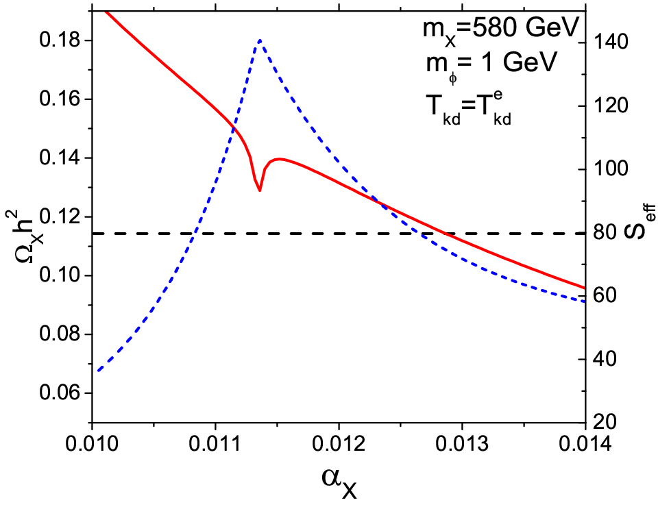
  We choose the maximal $\alpha_{X}$ that yields $\Omega_{X}h^{2}=0.114$. Roughly speaking, $\Omega_{X}h^{2}$ decreases as $\alpha_{X}$ increases, and so typically, there is a unique choice of $\alpha_{X}$ that yields the correct $\Omega_{X}h^{2}$. In some cases with strong resonances, however, there are three choices of $\alpha_{X}$ that give the correct $\Omega_{X}$, as shown in Fig. 3. When we do a coarse scan there is no guarantee that we always pick the solution with the largest value of $S_{\text{eff}}$. Note, however, that the values of $S_{\text{eff}}$ only change by about 20–30% between the three allowed solutions, and such variations do not modify our conclusions. The values of $\alpha_{X}$ that yield the correct relic density for given values of $m_{X}$ and $m_{\phi}$ are given in Fig. 4. Note that close to a resonance, one needs extreme fine-tuning to avoid efficient annihilation in the early Universe and obtain the correct relic density.

In Fig. 5, we show the maximal values of $S_{\text{eff}}$ as a function of $m_{X}$ for $m_{\phi}=250~\text{MeV}$ and 1 GeV. To understand the impact of resonances and the Sommerfeld effect on freeze out on these results, we also plot other Sommerfeld enhancements. $S^{0}$, which includes neither resonances nor freeze out effects, was used in Ref. [2]. We see that it is almost always overestimates the maximal Sommerfeld enhancement. This is because, as evident in Fig. 5, the effect of Sommerfeld enhanced annihilation on freeze out is a significant suppression. This may be understood as follows. If Sommerfeld enhancement reduces the thermal relic density by a factor $\zeta$, the tree-level cross section $(\sigma_{\text{an}}v_{\text{rel}})_{0}$ must be reduced by $\zeta$ to keep $\Omega_{X}$ fixed. However, $S_{\text{eff}}\propto\alpha_{X}^{3}\propto(\sigma_{\text{an}}v_{\text{rel}})_{0}^{3/2}$, and so reducing $\Omega_{X}$ by $\zeta$ implies a reduction in $S_{\text{eff}}$ by a factor $\zeta^{3/2}$. For example, for $m_{X}=1~\text{TeV}$, the maximal coupling is $\alpha_{X}\simeq 0.021$, and $\zeta\sim 1.5$, consistent with the results of Refs. [29, 30]. Including the effect of freeze out here therefore reduces $S^{0}$ to $S_{\text{eff}}^{0}$ by a factor of $(1.5)^{3/2}\sim 2$, a significant reduction.

Adding resonances then produces oscillations about the $S^{0}$ and $S_{\text{eff}}^{0}$ contours, with peak positions given by Eq. (7). We see that, although resonances can significantly enhance the effective Sommerfeld factor, these enhancements are significant only for low values of $n$; for $m_{\phi}\lesssim\text{GeV}$, these lie at low $m_{X}$, and the effect becomes negligible for $m_{X}\gtrsim 1~\text{TeV}$.

In Fig. 5, we have fixed $m_{\phi}$ to typical values considered in the literature. In Fig. 6, we plot upper bounds on $S_{\text{eff}}$ as a function of $m_{\phi}$ for fixed values of $m_{X}$. We see that the resonances have little impact for $m_{\phi}\lesssim 1~\text{GeV}$, but can produce enhancements by factors of 2 to 3 for larger $m_{\phi}$. Large values of $m_{\phi}\gtrsim 1~\text{GeV}$ have been considered disfavored, however, as they eliminate the kinematic suppression of anti-proton fluxes, which are typically considered to be consistent with astrophysical backgrounds.

What is the effect on $S_{\text{eff}}$ of deviating from the $S_{\text{eff}}$-maximizing assumptions? The effect of the choice of $T_{\text{kd}}$ is highly sensitive to how close one is to a resonance. Far from a resonance, there is little sensitivity to $T_{\text{kd}}$ values between $T_{\text{kd}}^{\phi}$ and $T_{\text{kd}}^{e}$. As one approaches a resonance, however, $S_{\text{eff}}$ may vary by $\sim 10\%$ or more. In particular, we found regions close to resonances for $m_{\phi}\sim\text{GeV}$ where $S_{\text{eff}}$ changed by about 30%. This behavior is shown in Fig. 7. If one is not very close to a resonance, the choice of $x_{\text{s}}$ has a small impact. In contrast, as discussed above, the assumption of $\Omega_{X}h^{2}=0.114$ has a large effect; for other choices, the maximal value of $S_{\text{eff}}$ scales as $(\Omega_{X}h^{2})^{3/2}$. Finally, as can be seen in Fig. 3, different choices of $\alpha_{X}$ also decrease $S_{\text{eff}}\propto\alpha_{X}^{3}$ by $\sim 20-30\%$.

For typical parameters that are not very close to a resonance, then, we expect that assumptions different from those listed above would produce a small decrease in $S_{\text{eff}}$ when away from resonances. Note, however, that very near a resonance, all of these choices become very important, as we now discuss.

Very near a resonance, the annihilation cross section becomes sensitive to details of the dark matter’s evolution to low velocities at late times. The effective Sommerfeld enhancement then becomes highly sensitive to details of $T_{\text{kd}}$, the velocity distribution of dark matter after $T_{\text{kd}}$, and the cutoff of resonant enhancements. As this is far from generic, we do not present details of these dependences, but we note that, contrary to naive expectations, $S_{\text{eff}}$ is not maximized by sitting exactly at resonance. In fact, exact resonances lead to extremely efficient annihilation in the early Universe and minimize current indirect signals.

Resonant Sommerfeld enhancement’s effect on freeze out can also be so large that it leads to the intriguing phenomenon of chemical recoupling. This is illustrated for two representative cases in Fig. 8. Without resonant Sommerfeld enhancement, dark matter freezes out and remains frozen out, but with resonant enhancement, dark matter may melt back in at late times, or chemically recouple, leading to a second era of efficient annihilation.

The phenomenon of chemical recoupling in the context of Sommerfeld enhancements may be understood as follows. The Hubble parameter scales as $H\sim T^{2}$. The annihilation rate is $\Gamma_{\text{an}}=n_{X}\langle\sigma_{\text{an}}v_{\text{rel}}\rangle$. The dark matter density scales as $n_{X}\sim T^{3}$, and $\langle\sigma_{\text{an}}v_{\text{rel}}\rangle$ scales as $v_{\text{rel}}^{-1}\sim T_{X}^{-1/2}$ off resonance and $v_{\text{rel}}^{-2}\sim T_{X}^{-1}$ on resonance. Before $T_{\text{kd}}$, $T_{X}=T$, and so the annihilation rate cannot grow relative to the expansion rate. However, after $T_{\text{kd}}$, $T_{X}\propto T^{2}$, and so $\Gamma_{\text{an}}\sim T$. At late times, then, the annihilation rate decrease slowly enough to become comparable to or greater than the expansion rate. The dark matter then melts back in, and there is a new era of annihilation. In these cases, the relic density is very sensitive to the temperature at which we stop including the annihilation process. As our default case, we have been conservative and stopped the annihilation process when the self-interactions of dark matter are no longer able to maintain kinetic equilibrium. Annihilations will proceed beyond this temperature; however, we cannot assume a Maxwellian distribution for the dark matter particle, because the annihilations preferentially deplete the low momentum tail. As an example, we show in Fig. 8 what happens when we allow the annihilation process to proceed down to 1 eV. The relic density is essentially negligible for the case where we have chemical recoupling, whereas it is unchanged for the case away from resonance.

In Figs. 9 and 10, we compare the maximal $S_{\text{eff}}$ presented in Fig. 5 to the boost factors required to explain PAMELA and Fermi data. The PAMELA and Fermi regions, derived in Ref. [20], assume an isothermal halo and a 250 MeV force carrier that decays with 100% branching ratio to $\mu^{+}\mu^{-}$, leading to annihilations $XX\to\mu^{+}\mu^{-}\mu^{+}\mu^{-}$. The fits are insensitive to $m_{\phi}$, provided $m_{\phi}\ll m_{X}$. The best fit is for $(m_{X},S_{\text{eff}})=(2.35~\text{TeV},1500)$, and the regions are $2\sigma$ contours relative to the best fit parameters. Results for other halo profiles, other particle physics models, and other final states have also been considered [20, 21, 46]. These studies find that the 4$\mu$ final state provides a better fit than all other considered final states, but see Sec. V.4 for a discussion of this issue.

Despite choosing $T_{\text{kd}}$ and all other parameters to maximize $S_{\text{eff}}$, we find that the possible values of $S_{\text{eff}}$ fall short of explaining the PAMELA and Fermi excesses. For example, at $m_{X}=2.35~\text{TeV}$ the maximal Sommerfeld enhancement is $S_{\text{eff}}\approx 100$, a factor of 15 below the best fit value. For lower $m_{X}$, the data may be fit with smaller $S_{\text{eff}}$, but the relic density bounds are also stronger; for example, for $m_{\phi}=250~\text{MeV}$ and $m_{X}=0.1$, 0.3, and 1 TeV, the maximal values of $S_{\text{eff}}$ are 7, 30, and 90, respectively.

Our analysis so far has assumed standard astrophysics and astroparticle physics. To enable Sommerfeld enhancements to explain PAMELA and Fermi, one may consider uncertainties in these assumptions.

The annihilation signal is sensitive to the square of the dark matter density $\rho_{X}$ in the local neighborhood. The best fit regions given in Ref. [20] assume the conventional value $\rho_{X}=0.3~\text{GeV}/\text{cm}^{3}$, which has traditionally been considered to be uncertain up to a factor of 2 [47]. More recently, studies have tried to refine the calculation of the uncertainty in the local density of dark matter. One study found $\rho_{X}=0.389\pm 0.025~\text{GeV}/\text{cm}^{3}$ [48], using an ensemble of kinematic tracers to constrain a standard galactic model with a spherical halo, stellar and gas disk and stellar bulge. Another recent study [49] finds $\rho_{X}=0.2-0.4~\text{GeV}/\text{cm}^{3}$. A third study Taylor-expanded the local rotation velocity curve to first order and used local kinematic tracers and an estimate of the baryonic contribution to the rotation curve to find $\rho_{X}=0.430\pm 0.113\pm 0.096~\text{GeV}/\text{cm}^{3}$ [50], where the first uncertainty is from the slope of the circular velocity $V(r)$ at the Sun’s radius and the second is from uncertainty in distance of the Sun from the galactic center. The three studies are consistent with each other, but the first one finds significantly smaller uncertainty in the value of $\rho_{X}$. If we use the results of Ref. [48], then the best fit regions plotted in Figs. 9 and 10 shift down by a factor of $(0.4/0.3)^{2}$. Of course, it is not appropriate to simply scale up the signal by some $\rho_{X}^{2}$ required to fit the positron and electron data; in a proper analysis, one should include the appropriate likelihood for $\rho_{X}$ and $\Omega_{X}h^{2}$. We have also discussed some of the uncertainties in the velocity distribution function and their effects in Section IV.1, and, as with $\rho_{X}$ and $\Omega_{X}h^{2}$, these uncertainties should be included in the full likelihood analysis.

Another effect that was pointed out recently [51] is that the positrons produced within the unseen bound subhalos out in the Milky Way dark matter halo could propagate to the local neighborhood and contribute to the PAMELA and Fermi signal. For the best fit point, this study found that about $30\%$ of the positrons in PAMELA could be due to annihilations in the subhalos [51]. Taking $\rho_{X}=0.4~\text{GeV}/\text{cm}^{3}$ and an enhancement factor of 30% from subhalos, the discrepancy is reduced from a factor of 15 to a factor of 4. We see that these changes are insufficient to reach the best fit regime, even if all the parameters are simultaneously pushed in the most optimistic direction. A more troubling aspect of this calculation is however the fact that the subhalos considered were those resolved by the Via Lactea II simulation. This implies that the much larger contribution from the lower mass subhalos would over produce the signal. Appealing to subhalos to ${\cal O}(1)$ changes to the required $S_{\text{eff}}$ is therefore unmotivated.

Finally, we may also appeal to small scale structure in the immediate local neighborhood to enhance the positron signals. Such a contribution is largely unconstrained by data, but present simulations, even without the deleterious effect of the disk of stars, do not predict large enhancements from such an effect [52]. A recent study [53] using the Via Lactea II simulation and including the Sommerfeld effect for annihilation in the local clumps found that the probability of finding a subhalo close enough to make an ${\cal O}(1)$ effect on the $e^{+}e^{-}$ flux above about 100 GeV is about 4% and that this contribution could be about 15% if the Via Lactea II subhalo mass function is extrapolated down to lower (unresolved) masses. Two points are worthy of further note here. First, these subhalo results are going to be crucially affected by the disk. The zeroth order expectation is that the gravity of the stellar disk will not allow such subhalos to survive or even if they do, truncate it significantly. Second, for small $m_{\phi}$ and near resonances self-interactions are important [2, 41] and that could modify the internal structure of the subhalo as well as the mass function.

A more complicated set of astrophysical uncertainties is related to astrophysical backgrounds and the signals themselves. For example, the required Sommerfeld enhancement may be reduced if conventional astrophysical backgrounds have been under-estimated, cosmic ray propagation models are modified, pulsars contribute significantly to the positron flux, or the PAMELA $e^{+}$ sample includes some proton contamination. Any of these effects could reduce the required dark matter signal, but they could also plausibly eliminate the need for dark matter altogether, as has been argued in numerous studies [54, 55, 56, 57, 58, 59]. It is therefore typically unclear what the motivation would be for assuming that such effects account for part of the signal but not all of it, independent of a desire to leave room for a dark matter signal.

A possible exception to the above argument is the possibility of adjusting cosmic ray propagation models to match the Fermi spectrum. Such adjustments could remove the need to explain Fermi, without changing the PAMELA excess significantly [60]. As shown in Fig. 10, for $m_{X}\lesssim~\text{TeV}$ and $m_{\phi}\gtrsim 1~\text{GeV}$, the allowed Sommerfeld enhancements may be in marginal agreement with PAMELA data. This scenario is, however, problematic. A contribution to the $e^{\pm}$ flux at about 100 GeV to explain the observed PAMELA positron fraction implies a modification to the $e^{\pm}$ flux observed by Fermi. For example, a 500 GeV dark matter explanation for PAMELA with the correct relic density is marginally possible for $m_{\phi}=1~\text{GeV}$ according to the $4\mu$ fits of Ref. [21] as shown in Fig. 10. This would, however, imply a drop in the $e^{\pm}$ flux beyond 500 GeV, which is not seen by Fermi, a point stressed in previous works [21, 46]. Analysis of such a scenario with modified propagation models would be another avenue for further study.

In this section, we include bounds from the effect of residual annihilation at last scattering on the ionized electron fraction and therefore on the cosmic microwave background (CMB) power spectrum. The CMB bound may be written as [61, 62]

where $f$ is the average fraction of the energy produced in annihilation that reionizes Hydrogen between redshifts of 800 and 1000. For the $e^{\pm}$ final state, $f\simeq 0.7$, while for the $\mu^{\pm}$ final state, $f\simeq 0.25$ [62]. The left hand side $S|_{v=0}$ is the saturated Sommerfeld enhancement obtained by setting $v=0$ in Eq. (6). This is sufficient to approximate the Sommerfeld enhancement during recombination, unless one is right on top of a resonance, which is highly disfavored by this bound.

Equation (35) is not a monotonic function of $\alpha_{X}$. To impose this bound, we consider a region in $\alpha_{X}$ that is bounded by values 10% larger and smaller than the value of $\alpha_{X}$ dictated by the relic density bound of $\Omega_{X}h^{2}=0.114$. We find that large resonances are no longer allowed by the CMB bound as a comparison of Fig. 10 and Fig. 11 will show.

The best fit regions of the $(m_{X},S_{\text{eff}})$ plane shown in Figs. 9 and 10 assume that the force carrier decays solely to muons, leading to the $XX\to\phi\phi\to 4\mu$ annihilation channel. The $4\mu$ final state has been shown [20, 21, 63, 46] to be the final state that yields the best fit of all considered so far, as it leads to smooth $e^{\pm}$ distributions that can simultaneously explain both PAMELA and Fermi. At the same time, this is an inefficient mode, as significant energy is lost to neutrinos. To ameliorate the discrepancy between the required $S_{\text{eff}}$ to explain the anomalies and the maximal $S_{\text{eff}}$ allowed by the relic density constraint, one might consider other channels, which could potentially allow similar contributions to the $e^{\pm}$ spectrum with lower $S_{\text{eff}}$ and at lower $m_{X}$.

The existence of other decay channels is theoretically well-motivated and there are many possibilities. If the decay $\phi\to\mu^{+}\mu^{-}$ is possible, the decay $\phi\to e^{+}e^{-}$ is also kinematically allowed. For $m_{\phi}\sim 1~\text{GeV}$, other decay modes, such as $\phi\to\pi\pi,K\bar{K}$, are also possible. As an example, if $\phi$ decays are controlled by its kinetic mixing with the standard model photon, then there will also be $e^{\pm}$ and $\pi^{\pm}$ channels with roughly similar branching ratios, depending on $m_{\phi}$ [64]. Alternatively, $\phi$ particles may decay preferentially to the heaviest available states if they are coupled through standard model Yukawa couplings, or may have other interesting dynamics. In fact, in full generality, the $\phi$ particles may decay not only to pairs of standard model particles, but also through final states involving hidden Higgs bosons and other hidden particles, leading, for example, to $XX$ annihilations to 6 or 8 particle final states.

Studies so far have found that the $4\mu$ mode is a better fit than other channels [21, 63]. A precise quantitative statement requires inclusion of correlations through covariance matrices for each experiment, and these are not available. Given this fundamental uncertainty, conclusions about the $\mu$ mode and other channels are far from firm and require additional assumptions.

In Ref. [63], the $4e$ mode is shown to have a $\chi^{2}/\text{dof}$ that is larger by about $\sim 1$ compared the $4\mu$ mode. These values of $\chi^{2}$ are computed by assuming that the data points are uncorrelated and allowing for the spatial diffusion parameter to vary. Other results obtained by fixing the diffusion parameter seem to agree qualitatively with this result [21]. In fact, marginalizing over $m_{X}$ and other parameters, Ref. [21] found that the possibility of mixed modes in the ratio of $4e:4\mu=1:1$ is excluded at 99.9% CL.

Despite these results, we may consider what impact other modes might have, especially in light of the fact that there is a lot of freedom in the cosmic ray propagation model parameters. As an illustration, we consider the best fit regions from Ref. [21] for both the $4e$ and $4\mu$ modes separately. We plot these best fit regions with the relic density and CMB upper limits on $S_{\text{eff}}$ in Fig. 11. The best-fit point for the $4e$ mode is at lower $S_{\text{eff}}$ and $m_{X}$ and the edge of the region is in marginal agreement with the relic density constraint. Of course, as discussed above, the best-fit point for the $4e$ mode has a much lower likelihood than the best-fit point for the $4\mu$ mode, according to Ref. [21]. For a 1:1 ratio, the best fit point would move to $X$ masses somewhere between 1.5 and 2 TeV. This is disfavored by the relic density requirement even if we set the local dark matter density to be $0.4~\text{GeV}/\text{cm}^{3}$.

For the reasons noted above, all of these conclusions are subject to many uncertainties. The present conclusion in the literature seems to that significant deviations from the pure $4\mu$ channel do not provide a good fit to data. One way forward would be to redo fits of the kind discussed in literature, allowing for variations in cosmic ray propagation model parameters to see if this conclusion holds up in general. In any case, a careful statistical analysis is required before appeals to alternative channels alone may be considered as a way to allow Sommerfeld scenarios to explain the data.

For the case of attractive forces, pairs of dark matter particles may form bound states by radiating force carrier particles if the force carrier mass $m_{\phi}$ is below the binding energy $\alpha_{X}^{2}m_{X}/4$ [18, 65, 66]. As in the case of positronium, when this is kinematically possible, annihilation through bound states is preferred. In the limits $m_{\phi}\ll\alpha_{X}^{2}m_{X}/4$ and $v\gg m_{\phi}/m_{X}$, the annihilation rate enhancement is about $20\alpha_{X}v_{\phi}(3-v_{\phi}^{2})/(2v)$ for fermions, where $v_{\phi}$ is the velocity of the final state $\phi$ particle when the bound state forms [18]. This is roughly a factor of 7 larger than $S^{0}$ when $v_{\phi}\simeq 1$.

Unfortunately, such bound state effects do not help Sommerfeld enhancement models explain the PAMELA and Fermi data for two reasons. First, bound state formation is kinematically forbidden in large parts of parameter space that yield the best fits to data, and the large factor of 7 enhancement alluded to above is not realized for most of the parameter space plotted in Fig. 10. To see this, we first need to compute the value of $\alpha_{X}$ required to get the right relic density. Now, bound states may form in the early Universe when they are energetically viable, that is when $v<\alpha_{X}$, and hence affect the relic density calculation. For simplicity we neglect this effect here, and use the same $\alpha_{X}$ values from Fig. 4, which leads to a conservative bound. Then, for $m_{\phi}=0.25~\text{GeV}\ (1~\text{GeV})$, the bound state enhancement formula quoted above is valid only for $m_{X}\gg 1.5~\text{TeV}\ (2.5~\text{TeV})$. These inequalities are not satisfied for parameters that are most promising for fitting the data ($m_{\phi}\gtrsim 0.25~\text{GeV}$ and $m_{X}\lesssim 4~\text{TeV}$).

Second, if bound states form, they are likely to be in conflict with bounds from the CMB. To see this, let’s saturate the bound state enhancement at $v\sim m_{\phi}/m_{X}$ and estimate the enhancement at recombination as $20\alpha_{X}m_{X}/m_{\phi}$. This should be compared to the CMB bound of $(120/f)(m_{X}/\text{TeV})\simeq 500~(m_{X}/\text{TeV})$, where we have set $f=0.25$ to be conservative. To satisfy the CMB bound, then, we require $\alpha_{X}<(m_{\phi}/\text{GeV})/40$. This is generically violated if $\alpha_{X}$ is fixed by the relic density. For example, for $m_{\phi}=1~\text{GeV}$, the bound implies $\alpha_{X}<0.025$. Requiring the correct relic density then implies $m_{X}<1~\text{TeV}$. However, we need $m_{X}>2.5~\text{TeV}$ for bound states to form with $m_{\phi}=1~\text{GeV}$. The situation is no different with $m_{\phi}=0.25~\text{GeV}$. Thus our saturation approximation above (for bound state enhancement) suggests that regions of parameter spaces where bound states can form are generically in conflict with the CMB.

A potentially more promising direction is to construct more complicated particle physics models to achieve Sommerfeld enhancements that are large enough to explain PAMELA and Fermi. Such models will generically include additional annihilation channels. We begin by discussing the impact of these channels in general, and then examine various strategies one might explore to achieve larger $S_{\text{eff}}$.

References

- [1] H. Goldberg, Phys. Rev. Lett. 50, 1419 (1983) [Erratum-ibid. 103, 099905 (2009)].
- [2] J. L. Feng, M. Kaplinghat and H. B. Yu, Phys. Rev. Lett. 104, 151301 (2010) [arXiv:0911.0422 [hep-ph]].
- [3] S. W. Barwick et al. [HEAT Collaboration], Astrophys. J. 482, L191 (1997) [arXiv:astro-ph/9703192].
- [4] J. J. Beatty et al., Phys. Rev. Lett. 93, 241102 (2004) [arXiv:astro-ph/0412230].
- [5] O. Adriani et al. [PAMELA Collaboration], Nature 458, 607 (2009) [arXiv:0810.4995 [astro-ph]].
- [6] J. Chang et al. [ATIC Collaboration], Nature 456, 362 (2008).
- [7] A. A. Abdo et al. [The Fermi LAT Collaboration], Phys. Rev. Lett. 102, 181101 (2009) [arXiv:0905.0025 [astro-ph.HE]].
- [8] A. W. Strong et al., arXiv:0907.0559 [astro-ph.HE].
- [9] A. Sommerfeld, Annalen der Physik 403, 257 (1931).
- [10] H. Baer, K. m. Cheung and J. F. Gunion, Phys. Rev. D 59, 075002 (1999) [arXiv:hep-ph/9806361].
- [11] J. Hisano, S. Matsumoto and M. M. Nojiri, Phys. Rev. D 67 (2003) 075014 [arXiv:hep-ph/0212022].
- [12] J. Hisano, S. Matsumoto and M. M. Nojiri, Phys. Rev. Lett. 92, 031303 (2004) [arXiv:hep-ph/0307216].
- [13] J. Hisano, S. Matsumoto, M. M. Nojiri and O. Saito, Phys. Rev. D 71, 063528 (2005) [arXiv:hep-ph/0412403].
- [14] J. Hisano, S. Matsumoto, O. Saito and M. Senami, Phys. Rev. D 73, 055004 (2006) [arXiv:hep-ph/0511118].
- [15] M. Cirelli, A. Strumia and M. Tamburini, Nucl. Phys. B 787, 152 (2007) [arXiv:0706.4071 [hep-ph]].
- [16] M. Cirelli, M. Kadastik, M. Raidal and A. Strumia, Nucl. Phys. B 813, 1 (2009) [arXiv:0809.2409 [hep-ph]].
- [17] N. Arkani-Hamed, D. P. Finkbeiner, T. R. Slatyer and N. Weiner, Phys. Rev. D 79, 015014 (2009) [arXiv:0810.0713 [hep-ph]].
- [18] M. Pospelov, A. Ritz, Phys. Lett. B671, 391-397 (2009) [arXiv:0810.1502 [hep-ph]].
- [19] P. J. Fox and E. Poppitz, Phys. Rev. D 79, 083528 (2009) [arXiv:0811.0399 [hep-ph]].
- [20] L. Bergstrom, J. Edsjo and G. Zaharijas, Phys. Rev. Lett. 103, 031103 (2009) [arXiv:0905.0333 [astro-ph.HE]].
- [21] P. Meade, M. Papucci, A. Strumia and T. Volansky, Nucl. Phys. B 831, 178 (2010) [arXiv:0905.0480 [hep-ph]].
- [22] R. Iengo, JHEP 0905, 024 (2009) [arXiv:0902.0688 [hep-ph]].
- [23] R. Iengo, arXiv:0903.0317 [hep-ph].
- [24] S. Cassel, arXiv:0903.5307 [hep-ph].
- [25] T. R. Slatyer, JCAP 1002, 028 (2010) [arXiv:0910.5713 [hep-ph]].
- [26] J. Hisano, S. Matsumoto, M. Nagai, O. Saito and M. Senami, Phys. Lett. B 646, 34 (2007) [arXiv:hep-ph/0610249].
- [27] J. March-Russell, S. M. West, D. Cumberbatch and D. Hooper, JHEP 0807, 058 (2008) [arXiv:0801.3440 [hep-ph]].
- [28] Q. Yuan, X. J. Bi, J. Liu, P. F. Yin, J. Zhang and S. H. Zhu, JCAP 0912, 011 (2009) [arXiv:0905.2736 [astro-ph.HE]].
- [29] J. B. Dent, S. Dutta and R. J. Scherrer, Phys. Lett. B 687, 275 (2010) [arXiv:0909.4128 [astro-ph.CO]].
- [30] J. Zavala, M. Vogelsberger and S. D. M. White, Phys. Rev. D 81, 083502 (2010) [arXiv:0910.5221 [astro-ph.CO]].
- [31] P. Gondolo and G. Gelmini, Nucl. Phys. B 360, 145 (1991).
- [32] E. W. Kolb and M. S. Turner, Front. Phys. 69, 1 (1990).
- [33] B. Holdom, Phys. Lett. B 166, 196 (1986).
- [34] B. Batell, M. Pospelov and A. Ritz, Phys. Rev. D 79, 115008 (2009) [arXiv:0903.0363 [hep-ph]].
- [35] J. D. Bjorken, R. Essig, P. Schuster and N. Toro, Phys. Rev. D 80, 075018 (2009) [arXiv:0906.0580 [hep-ph]].
- [36] M. Pospelov, A. Ritz and M. B. Voloshin, Phys. Lett. B 662, 53 (2008) [arXiv:0711.4866 [hep-ph]].
- [37] J. L. Feng, H. Tu and H. B. Yu, JCAP 0810, 043 (2008) [arXiv:0808.2318 [hep-ph]].
- [38] D. P. Finkbeiner, T. R. Slatyer, N. Weiner and I. Yavin, JCAP 0909, 037 (2009) [arXiv:0903.1037 [hep-ph]].
- [39] J. L. Feng, M. Kaplinghat, H. Tu and H. B. Yu, JCAP 0907, 004 (2009) [arXiv:0905.3039 [hep-ph]].
- [40] L. Ackerman, M. R. Buckley, S. M. Carroll and M. Kamionkowski, Phys. Rev. D 79, 023519 (2009) [arXiv:0810.5126 [hep-ph]].
- [41] M. R. Buckley and P. J. Fox, Phys. Rev. D 81, 083522 (2010) [arXiv:0911.3898 [hep-ph]].
- [42] M. Ibe and H. B. Yu, Phys. Lett. B 692, 70 (2010) [arXiv:0912.5425 [hep-ph]].
- [43] S. A. Khrapak et al., Phys. Rev. Lett. 90, 225002 (2003).
- [44] S. A. Khrapak et al., IEEE Transactions on Plasma Science 32, 555 (2004).
- [45] X. X. Xue et al. [SDSS Collaboration], Astrophys. J. 684, 1143 (2008) [arXiv:0801.1232 [astro-ph]].
- [46] K. N. Abazajian, P. Agrawal, Z. Chacko and C. Kilic, arXiv:1002.3820 [astro-ph.HE].
- [47] M. Kamionkowski and A. Kinkhabwala, Phys. Rev. D 57, 3256 (1998) [arXiv:hep-ph/9710337].
- [48] R. Catena and P. Ullio, JCAP 1008, 004 (2010) [arXiv:0907.0018 [astro-ph.CO]].
- [49] M. Weber and W. de Boer, arXiv:0910.4272 [astro-ph.CO].
- [50] P. Salucci, F. Nesti, G. Gentile and C. F. Martins, arXiv:1003.3101 [astro-ph.GA].
- [51] J. M. Cline, A. C. Vincent and W. Xue, Phys. Rev. D 81, 083512 (2010) [arXiv:1001.5399 [astro-ph.CO]].
- [52] M. Vogelsberger et al., MNRAS 395, 797 (2009) [arXiv:0812.0362 [astro-ph]].
- [53] M. Kuhlen and D. Malyshev, Phys. Rev. D 79, 123517 (2009) [arXiv:0904.3378 [hep-ph]].
- [54] D. Hooper, P. Blasi and P. D. Serpico, JCAP 0901, 025 (2009) [arXiv:0810.1527 [astro-ph]].
- [55] H. Yuksel, M. D. Kistler and T. Stanev, Phys. Rev. Lett. 103, 051101 (2009) [arXiv:0810.2784 [astro-ph]].
- [56] S. Profumo, arXiv:0812.4457 [astro-ph].
- [57] S. Dado and A. Dar, Mem. Sci. Astron. Ital. 81, 132 (2010) [arXiv:0903.0165 [astro-ph.HE]].
- [58] P. L. Biermann, J. K. Becker, A. Meli, W. Rhode, E. S. Seo and T. Stanev, Phys. Rev. Lett. 103, 061101 (2009) [arXiv:0903.4048 [astro-ph.HE]].
- [59] B. Katz, K. Blum, J. Morag, and E. Waxman, MNRAS 405, 1458 (2010) [arXiv:0907.1686 [astro-ph.HE]].
- [60] D. Grasso et al. [FERMI-LAT Collaboration], Astropart. Phys. 32, 140 (2009) [arXiv:0905.0636 [astro-ph.HE]].
- [61] S. Galli, F. Iocco, G. Bertone and A. Melchiorri, Phys. Rev. D 80, 023505 (2009) [arXiv:0905.0003 [astro-ph.CO]].
- [62] T. R. Slatyer, N. Padmanabhan and D. P. Finkbeiner, Phys. Rev. D 80, 043526 (2009) [arXiv:0906.1197 [astro-ph.CO]].
- [63] V. Barger, Y. Gao, W. Y. Keung, D. Marfatia and G. Shaughnessy, Phys. Lett. B 678, 283 (2009) [arXiv:0904.2001 [hep-ph]].
- [64] A. Falkowski, J. T. Ruderman, T. Volansky and J. Zupan, JHEP 1005, 077 (2010) [arXiv:1002.2952 [hep-ph]].
- [65] J. D. March-Russell and S. M. West, Phys. Lett. B 676, 133 (2009) [arXiv:0812.0559 [astro-ph]].
- [66] W. Shepherd, T. M. P. Tait and G. Zaharijas, Phys. Rev. D 79, 055022 (2009) [arXiv:0901.2125 [hep-ph]].
- [67] D. Tucker-Smith and N. Weiner, Phys. Rev. D 64, 043502 (2001) [arXiv:hep-ph/0101138].
- [68] S. Chang, G. D. Kribs, D. Tucker-Smith and N. Weiner, Phys. Rev. D 79, 043513 (2009) [arXiv:0807.2250 [hep-ph]].
- [69] D. P. Finkbeiner and N. Weiner, Phys. Rev. D 76, 083519 (2007) [arXiv:astro-ph/0702587].
- [70] I. Cholis, L. Goodenough and N. Weiner, Phys. Rev. D 79, 123505 (2009) [arXiv:0802.2922 [astro-ph]].
- [71] K. M. Zurek, Phys. Rev. D 79, 115002 (2009) [arXiv:0811.4429 [hep-ph]].
- [72] A. Katz and R. Sundrum, JHEP 0906, 003 (2009) [arXiv:0902.3271 [hep-ph]].
- [73] I. Cholis and N. Weiner, arXiv:0911.4954 [astro-ph.HE].
- [74] F. Chen, J. M. Cline and A. R. Frey, Phys. Rev. D 80, 083516 (2009) [arXiv:0907.4746 [hep-ph]].
- [75] M. Cirelli and J. M. Cline, Phys. Rev. D 82, 023503 (2010) [arXiv:1005.1779 [hep-ph]].
- [76] G. Kane, R. Lu and S. Watson, Phys. Lett. B 681, 151 (2009) [arXiv:0906.4765 [astro-ph.HE]].
- [77] H. Zhang, C. S. Li, Q. H. Cao and Z. Li, arXiv:0910.2831 [hep-ph].
- [78] M. Kawasaki and T. Moroi, Astrophys. J. 452, 506 (1995) [arXiv:astro-ph/9412055].
- [79] R. H. Cyburt, J. R. Ellis, B. D. Fields and K. A. Olive, Phys. Rev. D 67, 103521 (2003) [arXiv:astro-ph/0211258].
- [80] M. Kamionkowski and S. Profumo, Phys. Rev. Lett. 101, 261301 (2008) [arXiv:0810.3233 [astro-ph]].
- [81] A. V. Belikov and D. Hooper, Phys. Rev. D 80, 035007 (2009) [arXiv:0904.1210 [hep-ph]].
- [82] S. Profumo and T. E. Jeltema, JCAP 0907, 020 (2009) [arXiv:0906.0001 [astro-ph.CO]].
- [83] G. Huetsi, A. Hektor and M. Raidal, Astron. Astrophys. 505, 999 (2009) [arXiv:0906.4550 [astro-ph.CO]].
- [84] M. Cirelli, F. Iocco and P. Panci, JCAP 0910, 009 (2009) [arXiv:0907.0719 [astro-ph.CO]].
- [85] T. Kanzaki, M. Kawasaki and K. Nakayama, Prog. Theor. Phys. 123, 853 (2010) [arXiv:0907.3985 [astro-ph.CO]].
- [86] R. M. Crocker, N. F. Bell, C. Balazs and D. I. Jones, Phys. Rev. D 81, 063516 (2010) [arXiv:1002.0229 [hep-ph]].
- [87] A. Calvez, W. Essey, M. Fairbairn, A. Kusenko and M. Loewenstein, arXiv:1003.1113 [astro-ph.HE].
- [88] S. Palomares-Ruiz and J. M. Siegal-Gaskins, JCAP 1007, 023 (2010) [arXiv:1003.1142 [astro-ph.CO]].