跳到论文正文
W Papers独立论文阅读器 arXiv:1005.4451 论文正文 计算阅读时间 · 0%
引用这篇论文根据当前论文元数据生成,正式投稿前建议核对。


License: arXiv.org perpetual non-exclusive license
arXiv:1005.4451v1 [hep-ph] 24 May 2010

Two-loop soft anomalous dimensions for single top quark associated production with a W−W^{-} or H−H^{-}

Nikolaos Kidonakis

Kennesaw State University, Physics #1202,
1000 Chastain Rd., Kennesaw, GA 30144-5591, USA

Abstract

I present results for the two-loop soft anomalous dimensions for associated production of a single top quark with a WW boson or a charged Higgs boson. The calculation uses expressions for the massive cusp anomalous dimension, which are presented in different forms, and it allows soft-gluon resummation at next-to-next-to-leading-logarithm (NNLL) accuracy. From the NNLL resummed cross section I derive approximate NNLO cross sections for b​g→t​W−bg\rightarrow tW^{-} and b​g→t​H−bg\rightarrow tH^{-} at LHC energies of 7, 10, and 14 TeV.

1 Introduction

The Large Hadron Collider (LHC) will produce top quarks via top-antitop pair or single top quark processes with relatively large cross sections. Given the importance of the top quark [1] to electroweak and Higgs physics, and the observation of single top events at the Tevatron [2, 3, 4], it is crucial to have a good theoretical understanding of top quark production cross sections. An interesting channel to study is associated production of a top quark with a WW boson, b​g→t​W−bg\rightarrow tW^{-}, which is sensitive to new physics and allows a direct measurement of the Vt​bV_{tb} CKM matrix element. This process is very small at the Tevatron but has the second highest cross section among single top processes at the LHC. A related process is associated production of a top quark with a charged Higgs boson, b​g→t​H−bg\rightarrow tH^{-}. Charged Higgs bosons appear in the Minimal Supersymmetric Standar Model (MSSM) and other two-Higgs-doublet models (2HDM). In the MSSM there are two Higgs doublets, one giving mass to the up-type fermions and the other to the down-type fermions. Among the extra Higgs particles in the MSSM are two charged Higgs bosons, H+H^{+} and H−H^{-}, and the associated production of a top quark with a charged Higgs is a process that the LHC has good potential to observe. Since a central mission of the LHC is to find the Higgs boson and another is to look for supersymmetry, the associated production of a charged Higgs with a top quark is an important channel to study.

The next-to-leading order (NLO) corrections to b​g→t​W−bg\rightarrow tW^{-} were calculated in [5] and to b​g→t​H−bg\rightarrow tH^{-} in [6, 7, 8]. These processes are very similar with respect to QCD corrections and they have the same color structure. Soft-gluon emission is an important contributor to higher-order corrections, particularly near partonic threshold. The soft-gluon corrections can be formally resummed to all orders in perturbation theory. The resummation follows from the factorization of the cross section into a hard-scattering function HH and a soft function SS that describes noncollinear soft-gluon emission in the process [9, 10]. The renormalization group evolution of the soft function is controlled by a process-dependent soft anomalous dimension ΓS\Gamma_{S}. The calculation of ΓS\Gamma_{S} is performed in the eikonal approximation, which describes the emission of soft gluons from partons in the hard scattering and leads to modified Feynman rules in diagram calculations. At next-to-leading-logarithm (NLL) accuracy these corrections were resummed for t​W−tW^{-} production at the Tevatron and at the LHC in [10, 11, 12], while the corrections for t​H−tH^{-} production were presented in [13, 14]. These results involved the calculations of the one-loop soft anomalous dimension for these processes.

Recent developments in two-loop calculations [15, 16, 17] have now made possible the resummation of next-to-next-to-leading-logarithm (NNLL) corrections for QCD processes. Here we begin by calculating the two-loop soft (cusp) anomalous dimension for two massive quarks, and then using these results in the limit when one quark is massive (top quark) and one is massless (bottom quark) we calculate the diagrams for associated single top quark production. Since there are three colored partons in the partonic processes b​g→t​W−bg\rightarrow tW^{-} and b​g→t​H−bg\rightarrow tH^{-} there are many diagrams to consider but the end result for the two-loop soft anomalous dimension for these processes can be written in a simple formula. We then use those results to calculate approximate next-to-next-to-leading order (NNLO) cross sections for t​W−tW^{-} and t​H−tH^{-} production at the LHC.

2 Two-loop soft (cusp) anomalous dimension for a heavy quark-antiquark pair

We begin by presenting the calculation of the two-loop cusp anomalous dimension, which is the soft anomalous dimension for e+​e−→t​t¯e^{+}e^{-}\rightarrow t{\bar{t}} [15, 16].

We expand the soft (cusp) anomalous dimension as ΓS=(αs/π)​ΓS(1)+(αs/π)2​ΓS(2)+⋯\Gamma_{S}=(\alpha_{s}/\pi)\Gamma_{S}^{(1)}+(\alpha_{s}/\pi)^{2}\Gamma_{S}^{(2)}+\cdots, The one-loop soft anomalous dimension, ΓS(1)\Gamma_{S}^{(1)}, can be read off the coefficient of the ultraviolet (UV) poles of the one-loop diagrams in Fig. 1.

In the eikonal approximation, as the gluon momentum goes to zero, the quark-gluon vertex reduces to gs​TFc​vμ/v⋅kg_{s}T_{F}^{c}\,v^{\mu}/v\cdot k, with gsg_{s} the strong coupling, vv a dimensionless velocity vector, kk the gluon momentum, and TFcT_{F}^{c} the generators of SU(3) in the fundamental representation. For example the integral for the diagram in Fig. 1(a) is given by

αsπ​I1​a=gs2​∫dn​k(2​π)n​(−i)​gμ​νk2​viμvi⋅k​(−vjν)(−vj⋅k)\frac{\alpha_{s}}{\pi}\,I_{1a}=g_{s}^{2}\int\frac{d^{n}k}{(2\pi)^{n}}\frac{(-i)g_{\mu\nu}}{k^{2}}\frac{v_{i}^{\mu}}{v_{i}\cdot k}\,\frac{(-v_{j}^{\nu})}{(-v_{j}\cdot k)} (2.1)

where ii labels the quark and jj the antiquark. The quark and antiquark velocity vectors obey the relations vi⋅vj=(1+β2)/2v_{i}\cdot v_{j}=(1+\beta^{2})/2 and vi2=vj2=(1−β2)/2v_{i}^{2}=v_{j}^{2}=(1-\beta^{2})/2, where β=1−4​m2/s\beta=\sqrt{1-4m^{2}/s} with mm the heavy quark mass and ss the center-of-mass energy squared. The eikonal diagrams are calculated in dimensional regularization with n=4−ϵn=4-\epsilon using Feynman gauge in momentum space.

Refer to caption
Figure 1: One-loop cusp diagrams with heavy-quark eikonal lines.

We find the one-loop soft (cusp) anomalous dimension

ΓS(1)=CF​[−(1+β2)2​β​ln⁡(1−β1+β)−1]\Gamma_{S}^{(1)}=C_{F}\left[-\frac{(1+\beta^{2})}{2\beta}\ln\left(\frac{1-\beta}{1+\beta}\right)-1\right] (2.2)

where CF=(Nc2−1)/(2​Nc)C_{F}=(N_{c}^{2}-1)/(2N_{c}) with Nc=3N_{c}=3 the number of colors. This result can also be written in terms of the cusp angle [18] γ=ln⁡[(1+β)/(1−β)]\gamma=\ln[(1+\beta)/(1-\beta)], with coth⁡γ=(1+β2)/(2​β)\coth\gamma=(1+\beta^{2})/(2\beta), as

ΓS(1)=CF​(γ​coth⁡γ−1).\Gamma_{S}^{(1)}=C_{F}(\gamma\coth\gamma-1)\,. (2.3)
Refer to caption
Figure 2: Two-loop cusp vertex diagrams with heavy-quark eikonal lines.
Refer to caption
Figure 3: Two-loop cusp self-energy diagrams with heavy-quark eikonal lines.
Refer to caption
Figure 4: Detail of the black blob of Fig. 3(a).

We now continue with the two-loop diagrams. In Fig. 2 we show graphs with vertex corrections and in Fig. 3 graphs with heavy-quark self-energy corrections. The dark blobs in Figs. 2(c) and 3(b) denote quark, gluon, and ghost loops. The black blob in Fig. 3(a) denotes three kinds of corrections shown in Fig. 4. We do not show graphs with gluon loops involving four-gluon vertices and graphs involving three-gluon vertices with all three gluons attaching to a single eikonal line since such graphs have vanishing contributions. For each diagram we include the appropriate one-loop counterterms for the divergent subdiagrams. The calculations are challenging because of the presence of the heavy quark mass. Dimensionally-regularized integrals needed in the calculation are shown in Appendix A. Using the results in Appendix A, the UV poles of the integrals for each diagram are provided in Appendix B.

Combining the kinematic results in Appendix B with color and symmetry factors, the contribution of the diagrams in Figs. 2 and 3 to the two-loop soft (cusp) anomalous dimension is

CF2​[I2​a+I2​b+2​I2​d+2​I2​e+I3​a​1+I3​a​2+I3​c]\displaystyle C_{F}^{2}\left[I_{2a}+I_{2b}+2\,I_{2d}+2\,I_{2e}+I_{3a1}+I_{3a2}+I_{3c}\right] (2.4)
+\displaystyle+ CF​CA​[−12​I2​b+I2​f−I2​c​g−I2​e−I3​b​g−12​I3​a​2]+12​CF​[I2​c​q+I3​b​q]\displaystyle C_{F}\,C_{A}\left[-\frac{1}{2}I_{2b}+I_{2f}-I_{2cg}-I_{2e}-I_{3bg}-\frac{1}{2}I_{3a2}\right]+\frac{1}{2}C_{F}\left[I_{2cq}+I_{3bq}\right]
=\displaystyle= −12​ϵ2​(ΓS(1))2+β04​ϵ2​ΓS(1)−12​ϵ​ΓS(2)\displaystyle-\frac{1}{2\epsilon^{2}}\left(\Gamma_{S}^{(1)}\right)^{2}+\frac{\beta_{0}}{4\epsilon^{2}}\Gamma_{S}^{(1)}-\frac{1}{2\epsilon}\Gamma_{S}^{(2)}

where IkI_{k} denotes the integral for diagram kk, e.g. I2​dI_{2d} is the integral for diagram 2(d). Also I2​c​qI_{2cq} and I3​b​qI_{3bq} denote the quark-loop contribution in Figs. 2(c) and 3(b), respectively, while I2​c​gI_{2cg} and I3​b​gI_{3bg} denote the gluon-loop plus ghost-loop contributions to the respective diagrams. I3​a​1I_{3a1} denotes the sum of the graphs 3(a1i) and 3(a1ii) detailed in Fig. 4 while I3​a​2I_{3a2} is the integral for the last graph in Fig. 4. On the right-hand side of Eq. (2.4) in addition to the two-loop soft anomalous dimension, ΓS(2)\Gamma_{S}^{(2)}, which appears in the coefficient of the 1/ϵ1/\epsilon pole, there also appear terms from the exponentiation of the one-loop result and the running of the coupling which account for all the double poles of the graphs. Here β0=(11/3)​CA−2​nf/3\beta_{0}=(11/3)C_{A}-2n_{f}/3, with CA=NcC_{A}=N_{c} and nfn_{f} the number of light quark flavors. From Eq. (2.4) we solve for the two-loop soft (cusp) anomalous dimension:

ΓS(2)=K2​ΓS(1)+CF​CA​Mβ\Gamma_{S}^{(2)}=\frac{K}{2}\,\Gamma_{S}^{(1)}+C_{F}C_{A}M_{\beta} (2.5)

where

Mβ=12+ζ22+12​ln2⁡(1−β1+β)\displaystyle M_{\beta}=\frac{1}{2}+\frac{\zeta_{2}}{2}+\frac{1}{2}\ln^{2}\left(\frac{1-\beta}{1+\beta}\right)
−(1+β2)28​β2​[ζ3+ζ2​ln⁡(1−β1+β)+13​ln3⁡(1−β1+β)+ln⁡(1−β1+β)​Li2​((1−β)2(1+β)2)−Li3​((1−β)2(1+β)2)]\displaystyle\hskip-28.45274pt{}-\frac{(1+\beta^{2})^{2}}{8\beta^{2}}\left[\zeta_{3}+\zeta_{2}\ln\left(\frac{1-\beta}{1+\beta}\right)+\frac{1}{3}\ln^{3}\left(\frac{1-\beta}{1+\beta}\right)+\ln\left(\frac{1-\beta}{1+\beta}\right){\rm Li}_{2}\left(\frac{(1-\beta)^{2}}{(1+\beta)^{2}}\right)-{\rm Li}_{3}\left(\frac{(1-\beta)^{2}}{(1+\beta)^{2}}\right)\right]
−(1+β2)4​β[ζ2−ζ2ln(1−β1+β)+ln2(1−β1+β)−13ln3(1−β1+β)+2ln(1−β1+β)ln((1+β)24​β)\displaystyle\hskip-28.45274pt{}-\frac{(1+\beta^{2})}{4\beta}\left[\zeta_{2}-\zeta_{2}\ln\left(\frac{1-\beta}{1+\beta}\right)+\ln^{2}\left(\frac{1-\beta}{1+\beta}\right)-\frac{1}{3}\ln^{3}\left(\frac{1-\beta}{1+\beta}\right)+2\ln\left(\frac{1-\beta}{1+\beta}\right)\ln\left(\frac{(1+\beta)^{2}}{4\beta}\right)\right.
−Li2((1−β)2(1+β)2)].\displaystyle\hskip 42.67912pt\left.{}-{\rm Li}_{2}\left(\frac{(1-\beta)^{2}}{(1+\beta)^{2}}\right)\right]\,. (2.6)

We have written the two-loop result ΓS(2)\Gamma_{S}^{(2)} in Eq. (2.5) in the form of a term which is a multiple of the one-loop soft anomalous dimension ΓS(1)\Gamma_{S}^{(1)}, Eq. (2.2), plus a set of additional terms which have been denoted as MβM_{\beta}. Here ζ2=π2/6\zeta_{2}=\pi^{2}/6 and ζ3=1.2020569⋯\zeta_{3}=1.2020569\cdots. The well-known two-loop constant KK [19] is given by K=CA​(67/18−ζ2)−5​nf/9K=C_{A}(67/18-\zeta_{2})-5n_{f}/9. The color structure of ΓS(2)\Gamma_{S}^{(2)} involves only the factors CF​CAC_{F}C_{A} and CF​nfC_{F}n_{f}. Note that as β→1\beta\rightarrow 1, Mβ→(1−ζ3)/2M_{\beta}\rightarrow(1-\zeta_{3})/2.

The result in Eq. (2.5) can be written in terms of the cusp angle γ\gamma as

ΓS(2)\displaystyle\Gamma_{S}^{(2)} =\displaystyle= K2ΓS(1)+CFCA{12+ζ22+γ22−12coth2γ[ζ3−ζ2γ−γ33−γLi2(e−2​γ)−Li3(e−2​γ)]\displaystyle\frac{K}{2}\,\Gamma_{S}^{(1)}+C_{F}C_{A}\left\{\frac{1}{2}+\frac{\zeta_{2}}{2}+\frac{\gamma^{2}}{2}-\frac{1}{2}\coth^{2}\gamma\left[\zeta_{3}-\zeta_{2}\gamma-\frac{\gamma^{3}}{3}-\gamma\,{\rm Li}_{2}\left(e^{-2\gamma}\right)-{\rm Li}_{3}\left(e^{-2\gamma}\right)\right]\right. (2.7)
−12cothγ[ζ2+ζ2γ+γ2+γ33+2γln(1−e−2​γ)−Li2(e−2​γ)]},\displaystyle\hskip 71.13188pt\left.{}-\frac{1}{2}\coth\gamma\left[\zeta_{2}+\zeta_{2}\gamma+\gamma^{2}+\frac{\gamma^{3}}{3}+2\,\gamma\,\ln\left(1-e^{-2\gamma}\right)-{\rm Li}_{2}\left(e^{-2\gamma}\right)\right]\right\},

and is in agreement, but in a simpler and more explicit form, with the result for the cusp anomalous dimension of Ref. [18].

3 Two-loop soft anomalous dimension and NNLL resummation for b​g→t​W−bg\rightarrow tW^{-} and b​g→t​H−bg\rightarrow tH^{-}

Refer to caption
Figure 5: Leading-order diagrams for b​g→t​W−bg\rightarrow tW^{-}.

We now turn our attention to processes that involve a bottom quark, a gluon, and a top quark as the colored particles in the hard scattering, namely t​W−tW^{-} and t​H−tH^{-} production. The leading-order diagrams for b​g→t​W−bg\rightarrow tW^{-} are shown in Fig. 5; if one replaces the W−W^{-} by an H−H^{-} the graphs describe b​g→t​H−bg\rightarrow tH^{-}. We treat the bottom quark as massless [13]. In this section we calculate the two-loop soft anomalous dimension that will allow us to resum the soft-gluon contributions to NNLL accuracy.

Refer to caption
Figure 6: One-loop eikonal diagrams with bottom quark-gluon-top quark vertex.

In Fig. 6 we show the one-loop eikonal diagrams for these processes. Calculating the integrals associated with these diagrams we find the one-loop soft anomalous dimension for b​g→t​W−bg\rightarrow tW^{-}:

ΓS,t​W−(1)=CF​[ln⁡(mt2−tmt​s)−12]+CA2​ln⁡(mt2−umt2−t)\Gamma_{S,\,tW^{-}}^{(1)}=C_{F}\left[\ln\left(\frac{m_{t}^{2}-t}{m_{t}\sqrt{s}}\right)-\frac{1}{2}\right]+\frac{C_{A}}{2}\ln\left(\frac{m_{t}^{2}-u}{m_{t}^{2}-t}\right) (3.1)

where s=(pb+pg)2s=(p_{b}+p_{g})^{2}, t=(pb−pt)2t=(p_{b}-p_{t})^{2}, u=(pg−pt)2u=(p_{g}-p_{t})^{2}, and mtm_{t} is the top quark mass. The expression for b​g→t​H−bg\rightarrow tH^{-} is identical. This result is slightly different from the result in Ref. [10, 13] because the axial gauge was used in those papers, while the result in Eq. (3.1) is calculated in Feynman gauge. Of course these differences are compensated by other terms in the resummed formula and the final result for the cross section is independent of the choice of gauge.

Refer to caption
Figure 7: Two-loop eikonal diagrams involving the bottom quark and gluon eikonal lines.
Refer to caption
Figure 8: Two-loop eikonal diagrams involving the bottom quark and top quark eikonal lines.
Refer to caption
Figure 9: Two-loop eikonal diagrams involving the gluon and top quark eikonal lines.

To find the two-loop soft anomalous dimension we calculate the diagrams shown in Figs. 7, 8, 9, plus diagrams involving the top-quark self energy as in Figs. 3 and 4. Since they are three colored partons, with one of them massive, we calculate diagrams that contribute to the cusp anomalous dimension for each pair of partons using the results in the previous section in the limit when one or both partons are massless. Note that diagrams that involve gluons attached to all three eikonal lines either vanish or do not contribute to the two-loop result [20], and hence we do not show them. Combining the kinematic results for the integrals from Appendix B with color and symmetry factors we have

CA24​[I2​a+2​I2​b+2​I2​c​g+2​I2​e−2​I2​f]b​t+CF2​[I2​a+I2​b+2​I2​d+2​I2​e+I3​a+I3​c]b​t\displaystyle\frac{C_{A}^{2}}{4}\left[I_{2a}+2\,I_{2b}+2\,I_{2cg}+2\,I_{2e}-2\,I_{2f}\right]_{bt}+C_{F}^{2}\left[I_{2a}+I_{2b}+2\,I_{2d}+2\,I_{2e}+I_{3a}+I_{3c}\right]_{bt} (3.2)
+\displaystyle+ CF​CA​[−I2​a−32​I2​b−I2​c​g−I2​d−2​I2​e+I2​f−I3​b​g−12​I3​a​2−12​I3​c]b​t−CA4​[I2​c​q]b​t\displaystyle C_{F}\,C_{A}\left[-I_{2a}-\frac{3}{2}I_{2b}-I_{2cg}-I_{2d}-2\,I_{2e}+I_{2f}-I_{3bg}-\frac{1}{2}I_{3a2}-\frac{1}{2}I_{3c}\right]_{bt}-\frac{C_{A}}{4}[I_{2cq}]_{bt}
+\displaystyle+ 12​CF​[I2​c​q+I3​b​q]b​t+CA24​[I2​a−2​I2​c​g+2​I2​d+2​I2​f]b​g+CA4​[I2​c​q]b​g\displaystyle\frac{1}{2}C_{F}\left[I_{2cq}+I_{3bq}\right]_{bt}+\frac{C_{A}^{2}}{4}\left[I_{2a}-2\,I_{2cg}+2\,I_{2d}+2\,I_{2f}\right]_{bg}+\frac{C_{A}}{4}[I_{2cq}]_{bg}
+\displaystyle+ CA24​[I2​a−2​I2​c​g+2​I2​d+2​I2​f]g​t+CA4​[I2​c​q]g​t+CF​CA​12​[I3​c]g​t+I3−line\displaystyle\frac{C_{A}^{2}}{4}\left[I_{2a}-2\,I_{2cg}+2\,I_{2d}+2\,I_{2f}\right]_{gt}+\frac{C_{A}}{4}[I_{2cq}]_{gt}+C_{F}C_{A}\frac{1}{2}[I_{3c}]_{gt}+I_{3-{\rm line}}
=\displaystyle= −12​ϵ2​(ΓS,t​W−(1))2+β04​ϵ2​ΓS,t​W−(1)−12​ϵ​ΓS,t​W−(2)\displaystyle-\frac{1}{2\epsilon^{2}}\left(\Gamma_{S,\,tW^{-}}^{(1)}\right)^{2}+\frac{\beta_{0}}{4\epsilon^{2}}\Gamma_{S,\,tW^{-}}^{(1)}-\frac{1}{2\epsilon}\Gamma_{S,\,tW^{-}}^{(2)}

where I3−lineI_{3-{\rm line}} denotes the terms involving gluons attached to all three lines that do not contribute at two loops and [I2​d]b​t[I_{2d}]_{bt}, for example, stands for the 2(d)-type diagram in Fig. 8 involving the bb and tt quarks.

We thus find the two-loop soft-anomalous dimension for b​g→t​W−bg\rightarrow tW^{-}

ΓS,t​W−(2)=K2​ΓS,t​W−(1)+CF​CA​(1−ζ3)4\Gamma_{S,\,tW^{-}}^{(2)}=\frac{K}{2}\Gamma_{S,\,tW^{-}}^{(1)}+C_{F}C_{A}\frac{(1-\zeta_{3})}{4}

where ΓS,t​W−(1)\Gamma_{S,\,tW^{-}}^{(1)} is given in Eq. (3.1). The result for b​g→t​H−bg\rightarrow tH^{-} is the same.

With the two-loop soft-anomalous dimension at hand we are now ready to resum the soft-gluon corrections at NNLL accuracy. For t​W−tW^{-} production the resummed partonic cross section in moment space (with NN the moment variable) is given by [9, 10, 17, 21]

σ^r​e​s​(N)\displaystyle{\hat{\sigma}}^{res}(N) =\displaystyle= exp⁡[Eq​(Nq)+Eg​(Ng)]​exp​[2​∫μFsd​μμ​(γq/q​(N~q,αs​(μ))+γg/g​(N~g,αs​(μ)))]\displaystyle\exp\left[E_{q}(N_{q})+E_{g}(N_{g})\right]\;\exp\left[2\int_{\mu_{F}}^{\sqrt{s}}\frac{d\mu}{\mu}\;\left(\gamma_{q/q}\left({\tilde{N}}_{q},\alpha_{s}(\mu)\right)+\gamma_{g/g}\left({\tilde{N}}_{g},\alpha_{s}(\mu)\right)\right)\right]\; (3.3)
×Hb​g→t​W−​(αs​(s))​Sb​g→t​W−​(αs​(s/N~′))​exp⁡[2​∫ss/N~′d​μμ​ΓS,t​W−​(αs​(μ))]\displaystyle\hskip-28.45274pt\times\,H^{bg\rightarrow tW^{-}}\left(\alpha_{s}(\sqrt{s})\right)\;S^{bg\rightarrow tW^{-}}\left(\alpha_{s}(\sqrt{s}/{\tilde{N}^{\prime}})\right)\;\exp\left[2\int_{\sqrt{s}}^{{\sqrt{s}}/{\tilde{N}^{\prime}}}\frac{d\mu}{\mu}\;\Gamma_{S,\,tW^{-}}\left(\alpha_{s}(\mu)\right)\right]

and similarly for t​H−tH^{-} production.

The first exponent [22, 23] in the above expression resums soft and collinear corrections from the incoming partons

Ei​(Ni)=∫01d​z​zNi−1−11−z​{∫1(1−z)2d​λλ​Ai​(αs​(λ​s))+Di​[αs​((1−z)2​s)]}E_{i}(N_{i})=\int^{1}_{0}dz\frac{z^{N_{i}-1}-1}{1-z}\;\left\{\int_{1}^{(1-z)^{2}}\frac{d\lambda}{\lambda}A_{i}\left(\alpha_{s}(\lambda s)\right)+D_{i}\left[\alpha_{s}((1-z)^{2}s)\right]\right\} (3.4)

where ii stands for the incoming bottom quark (i=qi=q) or the incoming gluon (i=gi=g). Here Nq=N⁡[(mW2−u)/mt2]N_{q}=N[(m_{W}^{2}-u)/m_{t}^{2}] and Ng=N⁡[(mW2−t)/mt2]N_{g}=N[(m_{W}^{2}-t)/m_{t}^{2}] where mWm_{W} is the WW-boson mass. The quantity AiA_{i} has a perturbative expansion, Ai=∑n(αs/π)n​Ai(n)A_{i}=\sum_{n}(\alpha_{s}/\pi)^{n}A_{i}^{(n)}. Here Aq(1)=CFA_{q}^{(1)}=C_{F} and Aq(2)=CF​K/2A_{q}^{(2)}=C_{F}K/2, while Ag(1)=CAA_{g}^{(1)}=C_{A} and Ag(2)=CA​K/2A_{g}^{(2)}=C_{A}K/2.

Also Di=∑n(αs/π)n​Di(n)D_{i}=\sum_{n}(\alpha_{s}/\pi)^{n}D_{i}^{(n)}, with Dq(1)=Dg(1)=0D_{q}^{(1)}=D_{g}^{(1)}=0, and [24]

Dq(2)=CF​CA​(−10154+116​ζ2+74​ζ3)+CF​nf​(727−ζ23)D_{q}^{(2)}=C_{F}C_{A}\left(-\frac{101}{54}+\frac{11}{6}\zeta_{2}+\frac{7}{4}\zeta_{3}\right)+C_{F}n_{f}\left(\frac{7}{27}-\frac{\zeta_{2}}{3}\right) (3.5)

and Dg(2)=(CA/CF)​Dq(2)D_{g}^{(2)}=(C_{A}/C_{F})D_{q}^{(2)}.

In the third exponent γi/i\gamma_{i/i} is the moment-space anomalous dimension of the MS¯{\overline{\rm MS}} parton density ϕi/i\phi_{i/i} and it controls the factorization scale, μF\mu_{F}, dependence of the cross section. We have γi/i=−Ai​ln⁡N~i+γi\gamma_{i/i}=-A_{i}\ln{\tilde{N}}_{i}+\gamma_{i} where AiA_{i} was defined above, N~i=Ni​eγE{\tilde{N}}_{i}=N_{i}e^{\gamma_{E}} with γE\gamma_{E} the Euler constant, and the parton anomalous dimension γi=∑n(αs/π)n​γi(n)\gamma_{i}=\sum_{n}(\alpha_{s}/\pi)^{n}\gamma_{i}^{(n)} where γq(1)=3​CF/4\gamma_{q}^{(1)}=3C_{F}/4 and γg(1)=β0/4\gamma_{g}^{(1)}=\beta_{0}/4.

Hb​g→t​WH^{bg\rightarrow tW} is the hard-scattering function while Sb​g→t​WS^{bg\rightarrow tW} is the soft function describing noncollinear soft gluon emission [9, 10]. The evolution of the soft function is controlled by the soft anomalous dimension ΓS,t​W−\Gamma_{S,\,tW^{-}}. Here N~′=N~​(s/mt2){\tilde{N}^{\prime}}={\tilde{N}}(s/m_{t}^{2}) with N~=N​eγE{\tilde{N}}=Ne^{\gamma_{E}}.

For t​H−tH^{-} production the resummed formula is essentially the same. The only difference, apart from the obvious use of the appropriate hard-scattering function for this process, is the definition of NqN_{q} and NgN_{g}. In this case, Nq=N⁡[(mH−2−u)/mH−2]N_{q}=N[(m_{H^{-}}^{2}-u)/m_{H^{-}}^{2}] and Ng=N⁡[(mH−2−t)/mH−2]N_{g}=N[(m_{H^{-}}^{2}-t)/m_{H^{-}}^{2}] where mH−m_{H^{-}} is the charged Higgs mass.

The resummed cross section, Eq. (3.3), can be expanded in the strong coupling, αs\alpha_{s}, and inverted to momentum space, thus providing fixed-order results for the soft-gluon corrections. The NLO expansion of the resummed cross section after inversion to momentum space is

σ^(1)=σB​αs​(μR)π​{c3​𝒟1​(s4)+c2​𝒟0​(s4)},{\hat{\sigma}}^{(1)}=\sigma^{B}\frac{\alpha_{s}(\mu_{R})}{\pi}\left\{c_{3}\,{\cal D}_{1}(s_{4})+c_{2}\,{\cal D}_{0}(s_{4})\right\}\,, (3.6)

where σB\sigma^{B} is the Born term for the process and μR\mu_{R} is the renormalization scale. We use the notation 𝒟k​(s4)=[lnk⁡(s4/mt2)/s4]+{\cal D}_{k}(s_{4})=[\ln^{k}(s_{4}/m_{t}^{2})/s_{4}]_{+} in t​W−tW^{-} production and 𝒟k​(s4)=[lnk⁡(s4/mH−2)/s4]+{\cal D}_{k}(s_{4})=[\ln^{k}(s_{4}/m_{H^{-}}^{2})/s_{4}]_{+} in t​H−tH^{-} production for the plus distributions involving logarithms of a kinematical variable s4s_{4} that measures distance from threshold (s4=0s_{4}=0 at threshold). For b​g→t​W−bg\rightarrow tW^{-}, s4=s+t+u−mt2−mW2s_{4}=s+t+u-m_{t}^{2}-m_{W}^{2}, while for b​g→t​H−bg\rightarrow tH^{-}, s4=s+t+u−mt2−mH−2s_{4}=s+t+u-m_{t}^{2}-m_{H^{-}}^{2}. The coefficient of the leading term is

c3=2​(Aq(1)+Ag(1)).c_{3}=2(A_{q}^{(1)}+A_{g}^{(1)})\,. (3.7)

The coefficient of the next-to-leading term, c2c_{2}, can be written as c2=c2μ+T2c_{2}=c_{2}^{\mu}+T_{2}, with c2μc_{2}^{\mu} denoting the terms involving logarithms of the scale and T2T_{2} denoting the scale-independent terms. For b​g→t​W−bg\rightarrow tW^{-}

c2μ=−(Aq(1)+Ag(1))​ln⁡(μF2mt2)c_{2}^{\mu}=-(A_{q}^{(1)}+A_{g}^{(1)})\ln\left(\frac{\mu_{F}^{2}}{m_{t}^{2}}\right) (3.8)

and

T2=−2​Aq(1)​ln⁡(mW2−umt2)−2​Ag(1)​ln⁡(mW2−tmt2)−(Aq(1)+Ag(1))​ln⁡(mt2s)+2​ΓS,t​W−(1).T_{2}=-2\,A_{q}^{(1)}\,\ln\left(\frac{m_{W}^{2}-u}{m_{t}^{2}}\right)-2\,A_{g}^{(1)}\,\ln\left(\frac{m_{W}^{2}-t}{m_{t}^{2}}\right)-(A_{q}^{(1)}+A_{g}^{(1)})\ln\left(\frac{m_{t}^{2}}{s}\right)+2\Gamma_{S,\,tW^{-}}^{(1)}\,. (3.9)

For b​g→t​H−bg\rightarrow tH^{-} replace both mWm_{W} and mtm_{t} in the above two equations by mH−m_{H^{-}}.

As discussed in [10, 13] the expansion can also determine the terms involving logarithms of the factorization and renormalization scales in the coefficient, c1c_{1}, of the δ⁡(s4)\delta(s_{4}) terms. If we denote these terms as c1μc_{1}^{\mu}, then for t​W−tW^{-} production

c1μ=[Aq(1)​ln⁡(mW2−umt2)+Ag(1)​ln⁡(mW2−tmt2)−γq(1)−γg(1)]​ln⁡(μF2mt2)+β04​ln⁡(μR2mt2),c_{1}^{\mu}=\left[A_{q}^{(1)}\,\ln\left(\frac{m_{W}^{2}-u}{m_{t}^{2}}\right)+A_{g}^{(1)}\,\ln\left(\frac{m_{W}^{2}-t}{m_{t}^{2}}\right)-\gamma_{q}^{(1)}-\gamma_{g}^{(1)}\right]\ln\left(\frac{\mu_{F}^{2}}{m_{t}^{2}}\right)+\frac{\beta_{0}}{4}\ln\left(\frac{\mu_{R}^{2}}{m_{t}^{2}}\right)\,, (3.10)

while for b​g→t​H−bg\rightarrow tH^{-} replace both mWm_{W} and mtm_{t} in the above equation by mH−m_{H^{-}}. The full virtual terms are not derivable from resummation, which addresses soft-gluon contributions, but can be taken from the complete NLO calculation.

The NNLO expansion of the resummed cross section for b​g→t​W−bg\rightarrow tW^{-} after inversion to momentum space is

σ^(2)\displaystyle{\hat{\sigma}}^{(2)} =\displaystyle= σBαs2​(μR)π2{12c32𝒟3(s4)+[32c3c2−β04c3]𝒟2(s4)\displaystyle\sigma^{B}\frac{\alpha_{s}^{2}(\mu_{R})}{\pi^{2}}\left\{\frac{1}{2}c_{3}^{2}\,{\cal D}_{3}(s_{4})+\left[\frac{3}{2}c_{3}c_{2}-\frac{\beta_{0}}{4}c_{3}\right]{\cal D}_{2}(s_{4})\right. (3.11)
+[c3​c1+c22−ζ2​c32−β02​T2+β04​c3​ln⁡(μR2mt2)+2​Aq(2)+2​Ag(2)]​𝒟1​(s4)\displaystyle\hskip-14.22636pt{}+\left[c_{3}c_{1}+c_{2}^{2}-\zeta_{2}c_{3}^{2}-\frac{\beta_{0}}{2}T_{2}+\frac{\beta_{0}}{4}c_{3}\ln\left(\frac{\mu_{R}^{2}}{m_{t}^{2}}\right)+2A_{q}^{(2)}+2A_{g}^{(2)}\right]{\cal D}_{1}(s_{4})
+[c2c1−ζ2c3c2+ζ3c32+β04c2ln(μR2s)−β02Aq(1)ln2(mW2−umt2)−β02Ag(1)ln2(mW2−tmt2)\displaystyle\hskip-14.22636pt{}+\left[c_{2}c_{1}-\zeta_{2}c_{3}c_{2}+\zeta_{3}c_{3}^{2}+\frac{\beta_{0}}{4}c_{2}\ln\left(\frac{\mu_{R}^{2}}{s}\right)\right.-\frac{\beta_{0}}{2}A_{q}^{(1)}\ln^{2}\left(\frac{m_{W}^{2}-u}{m_{t}^{2}}\right)-\frac{\beta_{0}}{2}A_{g}^{(1)}\ln^{2}\left(\frac{m_{W}^{2}-t}{m_{t}^{2}}\right)
−2​Aq(2)​ln⁡(mW2−umt2)−2​Ag(2)​ln⁡(mW2−tmt2)+Dq(2)+Dg(2)\displaystyle\hskip-14.22636pt\quad\quad{}-2A_{q}^{(2)}\ln\left(\frac{m_{W}^{2}-u}{m_{t}^{2}}\right)-2A_{g}^{(2)}\ln\left(\frac{m_{W}^{2}-t}{m_{t}^{2}}\right)+D_{q}^{(2)}+D_{g}^{(2)}
+β08(Aq(1)+Ag(1))ln2(μF2s)−(Aq(2)+Ag(2))ln(μF2s)+2ΓS,t​W−(2)]𝒟0(s4)}.\displaystyle\hskip-14.22636pt\quad\quad\left.\left.{}+\frac{\beta_{0}}{8}(A_{q}^{(1)}+A_{g}^{(1)})\ln^{2}\left(\frac{\mu_{F}^{2}}{s}\right)-(A_{q}^{(2)}+A_{g}^{(2)})\ln\left(\frac{\mu_{F}^{2}}{s}\right)+2\Gamma_{S,\,tW^{-}}^{(2)}\right]{\cal D}_{0}(s_{4})\right\}\,.

For b​g→t​H−bg\rightarrow tH^{-} again replace both mWm_{W} and mtm_{t} by mH−m_{H^{-}} in the above equation. It is important to note that all NNLO soft-gluon corrections are derived from the NNLL resummed cross section, i.e. the coefficients of all powers of logarithms in s4s_{4} are given in Eq. (3.11), from 𝒟3​(s4){\cal D}_{3}(s_{4}) down to 𝒟0​(s4){\cal D}_{0}(s_{4}). In Ref. [10] and [13, 14], where NLL accuracy was attained, only the coefficients of 𝒟3​(s4){\cal D}_{3}(s_{4}) and 𝒟2​(s4){\cal D}_{2}(s_{4}) were fully determined. Thus, at NNLL accuracy the theoretical improvement over NLL is significant. As discussed in [10, 14] additional δ⁡(s4)\delta(s_{4}) terms involving the factorization and renormalization scales are also computed.

4 NNLO approximate cross sections for t​W−tW^{-} and t​H−tH^{-} production at the LHC

NNLO approx (NNLL) t​W−tW^{-} cross section (pb)
mtm_{t} (GeV) LHC 7 TeV LHC 10 TeV LHC 14 TeV
170 8.24 20.3 43.6
171 8.09 20.0 43.0
172 7.94 19.7 42.4
173 7.80 19.4 41.8
174 7.66 19.1 41.2
175 7.53 18.7 40.6
Table 1: The b​g→t​W−bg\rightarrow tW^{-} production cross section in pb in p​ppp collisions at the LHC with S=7\sqrt{S}=7 TeV, 10 TeV, and 14 TeV, with μ=mt\mu=m_{t} and using the MSTW2008 NNLO pdf [26]. The approximate NNLO results are shown at NNLL accuracy.

We now use the results of the previous section to calculate approximate NNLO cross sections for b​g→t​W−bg\rightarrow tW^{-} and b​g→t​H−bg\rightarrow tH^{-} at the LHC.

We begin with t​W−tW^{-} production. As has been shown in [10, 11] the NLO expansion of the resummed cross section approximates well the complete NLO result for both Tevatron and LHC energies. In fact when damping factors are used to limit the soft-gluon contributions far away from threshold, as was also used for t​t¯t{\bar{t}} production [25] and ss-channel single-top production [17], then the approximation is excellent. This shows that soft-gluon corrections are dominant for this process.

In Table 1 we provide numerical values for the t​W−tW^{-} cross section at the LHC for energies of 7, 10, and 14 TeV and a range of top quark masses from 170 to 175 GeV. The NNLO approximate corrections increase the NLO cross section by ∼8\sim 8%. We note that the cross section for b¯​g→t¯​W+{\bar{b}}g\rightarrow{\bar{t}}W^{+} is identical.

At 7 TeV with mt=173m_{t}=173 GeV the approximate NNLO cross section from NNLL resummation is

σt​W−NNLOapprox​(mt=173​GeV, 7​TeV)=7.8±0.2​pb−0.6+0.5.\sigma^{\rm NNLOapprox}_{tW^{-}}(m_{t}=173\,{\rm GeV},\,7\,{\rm TeV})=7.8\pm 0.2{}^{+0.5}_{-0.6}\;{\rm pb}\,. (4.1)

The first uncertainty is from scale variation between mt/2m_{t}/2 and 2​mt2m_{t} and the second is from the MSTW2008 NNLO pdf at 90% C.L. At 10 TeV, again with mt=173m_{t}=173 GeV, the cross section is 19.4±0.5+1.0−1.119.4\pm 0.5{}^{+1.0}_{-1.1} pb, and at 14 TeV we find 41.8±1.0+1.5−2.441.8\pm 1.0{}^{+1.5}_{-2.4} pb.

Refer to caption
Figure 10: The cross section for t​W−tW^{-} production at the LHC with S=7\sqrt{S}=7 TeV, 10 TeV, and 14 TeV, and MSTW2008 NNLO pdf.

In Fig. 10 we plot the b​g→t​W−bg\rightarrow tW^{-} NNLO approximate cross section from NNLL resummation at the LHC versus top quark mass for energies of 7, 10, and 14 TeV.
Refer to caption
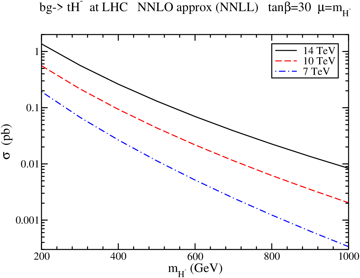
Figure 11: The cross section for t​H−tH^{-} production at the LHC with S=7\sqrt{S}=7 TeV, 10 TeV, and 14 TeV, and MSTW2008 NNLO pdf.

Next we consider the process b​g→t​H−bg\rightarrow tH^{-}. The ratio of the vacuum expectation values, v2,v1v_{2},v_{1} for the two Higgs doublets is tan⁡β=v2/v1\tan\beta=v_{2}/v_{1}, and the value of the cross section depends on the choice of this undetermined parameter. However, the overall percentage enhancement of the cross section from the higher-order soft-gluon corrections is independent of the value of tan⁡β\tan\beta.

In Fig. 11 we plot the b​g→t​H−bg\rightarrow tH^{-} NNLO approximate cross section from NNLL resummation at the LHC versus charged Higgs mass for energies of 7, 10, and 14 TeV, using a value of tan⁡β=30\tan\beta=30. The NNLO approximate corrections increase the NLO cross section by ∼15\sim 15% to ∼20\sim 20% for the range of charged Higgs masses shown. We note that the cross section for b¯​g→t¯​H+{\bar{b}}g\rightarrow{\bar{t}}H^{+} is identical (assuming the underlying model is C​PCP conserving).

5 Conclusion

The cross sections for associated production of a single top quark with a WW boson or with a charged Higgs boson receive large contributions from soft gluon corrections. These contributions were resummed in this paper to NNLL accuracy, thus extending previous NLL results. Attaining this accuracy requires the calculation of two-loop soft anomalous dimensions from the UV poles of dimensionally regularized integrals of two-loop eikonal diagrams. First the two-loop cusp anomalous dimension was calculated, which is an essential ingredient to all NNLL resummations for QCD processes, and then the result was used to calculate the two-loop soft anomalous dimensions for b​g→t​W−bg\rightarrow tW^{-} and b​g→t​H−bg\rightarrow tH^{-}. From the NNLL resummed formula approximate NNLO cross sections were derived and numerical predictions made for t​W−tW^{-} and t​H−tH^{-} production at LHC energies. These approximate NNLO corrections enhance the NLO cross section for t​W−tW^{-} production by ∼8\sim 8% and for t​H−tH^{-} production by ∼15\sim 15% to ∼20\sim 20%.

Acknowledgements

This work was supported by the National Science Foundation under Grant No. PHY 0855421.

Appendix A: Dimensionally regularized eikonal integrals

We list results for several dimensionally regularized integrals needed in the calculation of the two-loop soft anomalous dimension.

∫dn​kk2​vi⋅k​vj⋅k=iϵ​(−1)−1−ϵ2​π2−ϵ2​23+3​ϵ2​Γ​(1+ϵ2)​F12​(12,1+ϵ2,32,β2)\int\frac{d^{n}k}{k^{2}\,v_{i}\cdot k\,v_{j}\cdot k}=\frac{i}{\epsilon}(-1)^{-1-\frac{\epsilon}{2}}\pi^{2-\frac{\epsilon}{2}}2^{3+3\frac{\epsilon}{2}}\Gamma\left(1+\frac{\epsilon}{2}\right)\,{}_{2}F_{1}\left(\frac{1}{2},1+\frac{\epsilon}{2};\frac{3}{2};\beta^{2}\right) (A.1)

where F12{}_{2}F_{1} is the Gauss hypergeometric function.

∫dn​kk2​(vi⋅k)2=iϵ​(−1)1−ϵ2​π2−ϵ2​ 23+3​ϵ2​(1−β2)−1−ϵ2​Γ​(1+ϵ2)\int\frac{d^{n}k}{k^{2}\,(v_{i}\cdot k)^{2}}=\frac{i}{\epsilon}\,(-1)^{1-\frac{\epsilon}{2}}\,\pi^{2-\frac{\epsilon}{2}}\,2^{3+3\frac{\epsilon}{2}}(1-\beta^{2})^{-1-\frac{\epsilon}{2}}\Gamma\left(1+\frac{\epsilon}{2}\right) (A.2)
∫dn​k(k2)1+ϵ2​vi⋅k​vj⋅k=iϵ2​(−1)1−ϵβ​ 22​ϵ​π2−ϵ2​Γ​(1+ϵ)​1Γ⁡(1+ϵ2)\displaystyle\hskip-28.45274pt\int\frac{d^{n}k}{(k^{2})^{1+\frac{\epsilon}{2}}\,v_{i}\cdot k\,v_{j}\cdot k}=\frac{i}{\epsilon^{2}}\,\frac{(-1)^{1-\epsilon}}{\beta}\,2^{2\epsilon}\pi^{2-\frac{\epsilon}{2}}\,\Gamma(1+\epsilon)\frac{1}{\Gamma\left(1+\frac{\epsilon}{2}\right)}
×[(1−β)−ϵ​F12​(−ϵ,1+ϵ,1−ϵ,1−β2)−(1+β)−ϵ​F12​(−ϵ,1+ϵ,1−ϵ,1+β2)]\displaystyle\hskip-14.22636pt\times\left[(1-\beta)^{-\epsilon}{}_{2}F_{1}\left(-\epsilon,1+\epsilon;1-\epsilon;\frac{1-\beta}{2}\right){}-(1+\beta)^{-\epsilon}{}_{2}F_{1}\left(-\epsilon,1+\epsilon;1-\epsilon;\frac{1+\beta}{2}\right)\right] (A.3)
∫dn​kk2​(vi⋅k)1+ϵ​vj⋅k=i​π2−ϵ2ϵ⁡(1+ϵ)​22+9​ϵ2​(−1)−1−3​ϵ2​(1−β2)−1−3​ϵ2​Γ​(1+3​ϵ2)​1Γ⁡(1+ϵ)\displaystyle\hskip-25.60747pt\int\frac{d^{n}k}{k^{2}\,(v_{i}\cdot k)^{1+\epsilon}\,v_{j}\cdot k}=\frac{i\pi^{2-\frac{\epsilon}{2}}}{\epsilon(1+\epsilon)}2^{2+\frac{9\epsilon}{2}}(-1)^{-1-\frac{3\epsilon}{2}}(1-\beta^{2})^{-1-\frac{3\epsilon}{2}}\,\Gamma\left(1+\frac{3\epsilon}{2}\right)\frac{1}{\Gamma(1+\epsilon)}
×F1​[1+ϵ;1+3​ϵ2,1+3​ϵ2;2+ϵ;2​β1+β,−2​β1−β]\displaystyle\times F_{1}[1+\epsilon;1+\frac{3\epsilon}{2},1+\frac{3\epsilon}{2};2+\epsilon;\frac{2\beta}{1+\beta},\frac{-2\beta}{1-\beta}] (A.4)

where F1F_{1} is the Appell hypergeometric function.

∫dn​k2k22​[vi⋅(k1+k2)]2=iϵ​(−1)−1+ϵ2(1+ϵ)​ 24−ϵ2​π3−ϵ2​(1−β2)−1+ϵ2​(vi⋅k1)−ϵ\displaystyle\hskip-19.91692pt\int\frac{d^{n}k_{2}}{k_{2}^{2}\,\left[v_{i}\cdot(k_{1}+k_{2})\right]^{2}}=\frac{i}{\epsilon}\,\frac{(-1)^{-1+\frac{\epsilon}{2}}}{(1+\epsilon)}\,2^{4-\frac{\epsilon}{2}}\,\pi^{\frac{3-\epsilon}{2}}(1-\beta^{2})^{-1+\frac{\epsilon}{2}}\,(v_{i}\cdot k_{1})^{-\epsilon}\,
×Γ⁡(1+ϵ2)​Γ​(1−ϵ2)​Γ​(3+ϵ2)\displaystyle\quad\times\Gamma\left(1+\frac{\epsilon}{2}\right)\,\Gamma\left(1-\frac{\epsilon}{2}\right)\,\Gamma\left(\frac{3+\epsilon}{2}\right)\, (A.5)
∫dn​kk2​(vi⋅k)2+ϵ=i​π2−ϵ2ϵ⁡(1+ϵ)​22+9​ϵ2​(−1)−1−3​ϵ2​(1−β2)−1−3​ϵ2​Γ​(1+3​ϵ2)​1Γ⁡(1+ϵ)\int\frac{d^{n}k}{k^{2}\,(v_{i}\cdot k)^{2+\epsilon}}=\frac{i\pi^{2-\frac{\epsilon}{2}}}{\epsilon(1+\epsilon)}2^{2+\frac{9\epsilon}{2}}(-1)^{-1-\frac{3\epsilon}{2}}(1-\beta^{2})^{-1-\frac{3\epsilon}{2}}\,\Gamma\left(1+\frac{3\epsilon}{2}\right)\frac{1}{\Gamma(1+\epsilon)}\, (A.6)
∫dn​k1k12​vi⋅k1​vi⋅(k1+k2)=iϵ​(−1)ϵ2​ 22−ϵ2​π3−ϵ2​(vi⋅k2)−ϵ​(1−β2)−1+ϵ2\displaystyle\hskip-19.91692pt\int\frac{d^{n}k_{1}}{k_{1}^{2}\,v_{i}\cdot k_{1}\,v_{i}\cdot(k_{1}+k_{2})}=\frac{i}{\epsilon}\,(-1)^{\frac{\epsilon}{2}}\,2^{2-\frac{\epsilon}{2}}\,\pi^{\frac{3-\epsilon}{2}}(v_{i}\cdot k_{2})^{-\epsilon}\,(1-\beta^{2})^{-1+\frac{\epsilon}{2}}\,
×Γ⁡(1+ϵ2)​Γ​(1−ϵ2)​Γ​(ϵ−12)\displaystyle\quad\quad\times\Gamma\left(1+\frac{\epsilon}{2}\right)\,\Gamma\left(1-\frac{\epsilon}{2}\right)\,\Gamma\left(\frac{\epsilon-1}{2}\right)\, (A.7)
∫dn​k2k22​vi⋅k2​[vi⋅(k1+k2)]2=i1−ϵ​(−1)1+ϵ2​23−3​ϵ2​π2−ϵ2​(vi⋅k1)−1−ϵ\displaystyle\hskip-19.91692pt\int\frac{d^{n}k_{2}}{k_{2}^{2}\,v_{i}\cdot k_{2}\,[v_{i}\cdot(k_{1}+k_{2})]^{2}}=\frac{i}{1-\epsilon}\,(-1)^{1+\frac{\epsilon}{2}}2^{3-\frac{3\epsilon}{2}}\,\pi^{2-\frac{\epsilon}{2}}\,(v_{i}\cdot k_{1})^{-1-\epsilon}\,
×(1−β2)−1+ϵ2​Γ​(1−ϵ2)​Γ​(1+ϵ)\displaystyle\quad\quad\times(1-\beta^{2})^{-1+\frac{\epsilon}{2}}\,\Gamma\left(1-\frac{\epsilon}{2}\right)\,\Gamma(1+\epsilon)\, (A.8)
∫dn​k(k2)1+ϵ2​(vi⋅k)2=iϵ​(−1)−1−ϵ​ 22+3​ϵ​π2−ϵ2​(1−β2)−1−ϵ​Γ​(1+ϵ)​1Γ⁡(1+ϵ2)\int\frac{d^{n}k}{(k^{2})^{1+\frac{\epsilon}{2}}\,(v_{i}\cdot k)^{2}}=\frac{i}{\epsilon}\,(-1)^{-1-\epsilon}\,2^{2+3\epsilon}\,\pi^{2-\frac{\epsilon}{2}}(1-\beta^{2})^{-1-\epsilon}\,\Gamma(1+\epsilon)\,\frac{1}{\Gamma\left(1+\frac{\epsilon}{2}\right)}\, (A.9)

Appendix B: UV poles of the integrals for eikonal one-loop and two-loop diagrams for the soft (cusp) anomalous dimension

Here we present the UV poles of the integrals for the one-loop eikonal diagrams in Fig. 1 and the two-loop eikonal diagrams in Figs. 2 and 3.

First we list the integrals for the one-loop diagrams

I1​a=(1+β2)2​β​1ϵ​ln⁡(1−β1+β)I_{1a}=\frac{(1+\beta^{2})}{2\,\beta}\frac{1}{\epsilon}\ln\left(\frac{1-\beta}{1+\beta}\right) (B.1)

and

I1​b=1ϵI_{1b}=\frac{1}{\epsilon} (B.2)

Then we list the integrals for the two-loop diagrams:

I2​a+I2​b=(1+β2)28​β2​(−1)ϵ2​ln2⁡(1−β1+β).I_{2a}+I_{2b}=\frac{(1+\beta^{2})^{2}}{8\,\beta^{2}}\frac{(-1)}{\epsilon^{2}}\ln^{2}\left(\frac{1-\beta}{1+\beta}\right)\,. (B.3)
I2​b=(1+β2)28​β2​1ϵ​{−13​ln3⁡(1−β1+β)−ln⁡(1−β1+β)​[Li2​((1−β)2(1+β)2)+ζ2]+Li3​((1−β)2(1+β)2)−ζ3}I_{2b}=\frac{(1+\beta^{2})^{2}}{8\beta^{2}}\frac{1}{\epsilon}\left\{-\frac{1}{3}\ln^{3}\left(\frac{1-\beta}{1+\beta}\right)-\ln\left(\frac{1-\beta}{1+\beta}\right)\left[{\rm Li}_{2}\left(\frac{(1-\beta)^{2}}{(1+\beta)^{2}}\right)+\zeta_{2}\right]+{\rm Li}_{3}\left(\frac{(1-\beta)^{2}}{(1+\beta)^{2}}\right)-\zeta_{3}\right\}\\
I2​c​q=nf​(1+β2)6​β​[1ϵ2−56​ϵ]​ln⁡(1−β1+β)I_{2cq}=n_{f}\frac{(1+\beta^{2})}{6\,\beta}\left[\frac{1}{\epsilon^{2}}-\frac{5}{6\,\epsilon}\right]\ln\left(\frac{1-\beta}{1+\beta}\right) (B.4)
I2​c​g=524​(1+β2)β​[1ϵ2−3130​ϵ]​ln⁡(1−β1+β)I_{2cg}=\frac{5}{24}\frac{(1+\beta^{2})}{\beta}\left[\frac{1}{\epsilon^{2}}-\frac{31}{30\,\epsilon}\right]\ln\left(\frac{1-\beta}{1+\beta}\right) (B.5)
I2​d\displaystyle I_{2d} =\displaystyle= (1+β2)4​β{−1ϵ2ln(1−β1+β)+1ϵ[ln(1−β1+β)+12ln2(1−β1+β)\displaystyle\frac{(1+\beta^{2})}{4\beta}\left\{-\frac{1}{\epsilon^{2}}\ln\left(\frac{1-\beta}{1+\beta}\right)+\frac{1}{\epsilon}\left[\ln\left(\frac{1-\beta}{1+\beta}\right)+\frac{1}{2}\ln^{2}\left(\frac{1-\beta}{1+\beta}\right)\right.\right. (B.6)
+ln(1−β1+β)ln((1+β)24​β)−12Li2((1−β)2(1+β)2)+ζ22]}\displaystyle\left.\left.{}+\ln\left(\frac{1-\beta}{1+\beta}\right)\ln\left(\frac{(1+\beta)^{2}}{4\beta}\right)-\frac{1}{2}{\rm Li}_{2}\left(\frac{(1-\beta)^{2}}{(1+\beta)^{2}}\right)+\frac{\zeta_{2}}{2}\right]\right\}
I2​e=−I2​dI_{2e}=-I_{2d} (B.7)
I2​f=1ϵ​{−14​[2​ζ2+ln2⁡(1−β1+β)]​[(1+β2)2​β​ln⁡(1−β1+β)+1]+(1+β2)12​β​ln3⁡(1−β1+β)}\displaystyle I_{2f}=\frac{1}{\epsilon}\left\{-\frac{1}{4}\left[2\zeta_{2}+\ln^{2}\left(\frac{1-\beta}{1+\beta}\right)\right]\left[\frac{(1+\beta^{2})}{2\beta}\ln\left(\frac{1-\beta}{1+\beta}\right)+1\right]+\frac{(1+\beta^{2})}{12\beta}\ln^{3}\left(\frac{1-\beta}{1+\beta}\right)\right\} (B.8)
I3​a​1=−32​ϵ2+12​ϵ,I_{3a1}=-\frac{3}{2\epsilon^{2}}+\frac{1}{2\epsilon}, (B.9)
I3​a​2=1ϵ2−12​ϵI_{3a2}=\frac{1}{\epsilon^{2}}-\frac{1}{2\epsilon} (B.10)
I3​b​q=nf3​[1ϵ2−56​ϵ]I_{3bq}=\frac{n_{f}}{3}\left[\frac{1}{\epsilon^{2}}-\frac{5}{6\epsilon}\right] (B.11)
I3​b​g=512​[1ϵ2−3130​ϵ]I_{3bg}=\frac{5}{12}\left[\frac{1}{\epsilon^{2}}-\frac{31}{30\epsilon}\right] (B.12)
I3​c=−1ϵ2​(1+β2)2​β​ln⁡[(1−β)/(1+β)]I_{3c}=-\frac{1}{\epsilon^{2}}\frac{(1+\beta^{2})}{2\beta}\ln[(1-\beta)/(1+\beta)] (B.13)

In terms of the cusp angle

γ=ln⁡(vi⋅vj+(vi⋅vj)2−vi2​vj2vi2​vj2)\gamma=\ln\left(\frac{v_{i}\cdot v_{j}+\sqrt{(v_{i}\cdot v_{j})^{2}-v_{i}^{2}v_{j}^{2}}}{\sqrt{v_{i}^{2}v_{j}^{2}}}\right) (B.14)

and

coth⁡γ=vi⋅vj(vi⋅vj)2−vi2​vj2\coth\gamma=\frac{v_{i}\cdot v_{j}}{\sqrt{(v_{i}\cdot v_{j})^{2}-v_{i}^{2}v_{j}^{2}}} (B.15)

the previous results for the integrals can be written as

I1​a=−1ϵ​γ​coth⁡γI_{1a}=-\frac{1}{\epsilon}\gamma\coth\gamma (B.16)
I2​a+I2​b=−12​ϵ2​γ2​coth2⁡γI_{2a}+I_{2b}=-\frac{1}{2\epsilon^{2}}\gamma^{2}\coth^{2}\gamma (B.17)
I2​b=12​ϵ​coth2⁡γ⁡{γ⁡[Li2​(e−2​γ)+ζ2]+γ33+Li3​(e−2​γ)−ζ3}I_{2b}=\frac{1}{2\epsilon}\coth^{2}\gamma\left\{\gamma\left[{\rm Li}_{2}\left(e^{-2\gamma}\right)+\zeta_{2}\right]+\frac{\gamma^{3}}{3}+{\rm Li}_{3}\left(e^{-2\gamma}\right)-\zeta_{3}\right\} (B.18)
I2​c​q=nf3​γ​coth⁡γ⁡[−1ϵ2+56​ϵ]I_{2cq}=\frac{n_{f}}{3}\gamma\coth\gamma\left[-\frac{1}{\epsilon^{2}}+\frac{5}{6\epsilon}\right] (B.19)
I2​c​g=[−512​ϵ2+3172​ϵ]​γ​coth⁡γI_{2cg}=\left[-\frac{5}{12\epsilon^{2}}+\frac{31}{72\epsilon}\right]\gamma\coth\gamma (B.20)
I2​d=12​coth⁡γ⁡{1ϵ2​γ+1ϵ​[γ22−γ+γ​ln⁡(1−e−2​γ)−12​Li2​(e−2​γ)+ζ22]}I_{2d}=\frac{1}{2}\coth\gamma\left\{\frac{1}{\epsilon^{2}}\gamma+\frac{1}{\epsilon}\left[\frac{\gamma^{2}}{2}-\gamma+\gamma\ln\left(1-e^{-2\gamma}\right)-\frac{1}{2}{\rm Li}_{2}\left(e^{-2\gamma}\right)+\frac{\zeta_{2}}{2}\right]\right\} (B.21)
I2​f=1ϵ​{−14​[2​ζ2+γ2]​[−γ​coth⁡γ+1]−16​γ3​coth⁡γ}I_{2f}=\frac{1}{\epsilon}\left\{-\frac{1}{4}\left[2\zeta_{2}+\gamma^{2}\right]\left[-\gamma\coth\gamma+1\right]-\frac{1}{6}\gamma^{3}\coth\gamma\right\} (B.22)
I3​c=1ϵ2​γ​coth⁡γI_{3c}=\frac{1}{\epsilon^{2}}\gamma\coth\gamma (B.23)

The above expressions simplify when one of the quarks is massless. In that case coth⁡γ=1\coth\gamma=1 and

γ=ln⁡(2​vi⋅vjvi2​vj2)\gamma=\ln\left(\frac{2v_{i}\cdot v_{j}}{\sqrt{v_{i}^{2}v_{j}^{2}}}\right) (B.24)

The integrals listed before then take simpler forms:

I1​a=−1ϵ​γI_{1a}=-\frac{1}{\epsilon}\gamma (B.25)
I2​a+I2​b=−12​ϵ2​γ2I_{2a}+I_{2b}=-\frac{1}{2\epsilon^{2}}\gamma^{2} (B.26)
I2​b=12​ϵ[γ33+ζ2γ−ζ3}I_{2b}=\frac{1}{2\epsilon}\left[\frac{\gamma^{3}}{3}+\zeta_{2}\gamma-\zeta_{3}\right\} (B.27)
I2​c​q=nf3​γ​[−1ϵ2+56​ϵ]I_{2cq}=\frac{n_{f}}{3}\gamma\left[-\frac{1}{\epsilon^{2}}+\frac{5}{6\epsilon}\right] (B.28)
I2​c​g=[−512​ϵ2+3172​ϵ]​γI_{2cg}=\left[-\frac{5}{12\epsilon^{2}}+\frac{31}{72\epsilon}\right]\gamma (B.29)
I2​d=12​ϵ2​γ+12​ϵ​[γ22−γ+ζ22]I_{2d}=\frac{1}{2\epsilon^{2}}\gamma+\frac{1}{2\epsilon}\left[\frac{\gamma^{2}}{2}-\gamma+\frac{\zeta_{2}}{2}\right] (B.30)
I2​f=1ϵ​[112​γ3−14​γ2+ζ22​γ−ζ22]I_{2f}=\frac{1}{\epsilon}\left[\frac{1}{12}\gamma^{3}-\frac{1}{4}\gamma^{2}+\frac{\zeta_{2}}{2}\gamma-\frac{\zeta_{2}}{2}\right] (B.31)
I3​c=1ϵ2​γI_{3c}=\frac{1}{\epsilon^{2}}\gamma (B.32)

References

  • [1] W. Wagner, Rept. Prog. Phys. 68, 2409 (2005) [hep-ph/0507207]; A. Quadt, Eur. Phys. J. C 48, 835 (2006); R. Kehoe, M. Narain, and A. Kumar, Int. J. Mod. Phys. A 23, 353 (2008), arXiv:0712.2733 [hep-ex]; T. Han, Int. J. Mod. Phys. A 23, 4107 (2008), arXiv:0804.3178 [hep-ph]; W. Bernreuther, J. Phys. G 35, 083001 (2008), arXiv:0805.1333 [hep-ph]; D. Wackeroth, 0810.4176 [hep-ph]; M.-A. Pleier, Int. J. Mod. Phys. A 24, 2899 (2009), 0810.5226 [hep-ex]; J.R. Incandela, A. Quadt, W. Wagner, and D. Wicke, Prog. Part. Nucl. Phys. 63, 239 (2009), 0904.2499 [hep-ex]; W. Wagner, arXiv:1003.4359 [hep-ex].
  • [2] D0 Collaboration, V.M. Abazov et al., Phys. Rev. Lett. 103, 092001 (2009), arXiv:0903.0850 [hep-ex]; Phys. Lett. B 682, 363 (2010), arXiv:0907.4259 [hep-ex]; arXiv:0912.1066 [hep-ex].
  • [3] CDF Collaboration, T. Aaltonen et al., Phys. Rev. Lett. 103, 092002 (2009), arXiv:0903.0885 [hep-ex]; Phys. Rev. D 81, 072003 (2010), arXiv:1001.4577 [hep-ex]; arXiv:1004.1181 [hep-ex].
  • [4] E. Palencia, arXiv:0905.4279 [hep-ex]; D. Gillberg, arXiv:0906.0523 [hep-ex]; Tevatron Electroweak Working Group, arXiv:0908.2171 [hep-ex]; R. Schwienhorst, arXiv:0908.4553 [hep-ex]; A.P. Heinson, arXiv:0909.4518 [hep-ex]; C.E. Gerber, arXiv:0909.4794 [hep-ex]; L. Li, AIP Conf.Proc.1200, 666 (2010), arXiv:0911.1150 [hep-ex]; A.P. Heinson, Mod. Phys. Lett. A 25, 309 (2010), arXiv:1002.4167 [hep-ex].
  • [5] S.H. Zhu, Phys. Lett. B 524, 283 (2002) [hep-ph/0109269]; (E) B 537, 351 (2002).
  • [6] S.H. Zhu, Phys. Rev. D 67, 075006 (2003) [hep-ph/0112109].
  • [7] T. Plehn, Phys. Rev. D 67, 014018 (2003) [hep-ph/0206121].
  • [8] E.L. Berger, T. Han, J. Jiang, and T. Plehn, Phys. Rev. D 71, 115012 (2005) [hep-ph/0312286].
  • [9] N. Kidonakis and G. Sterman, Phys. Lett. B 387, 867 (1996); Nucl. Phys. B 505, 321 (1997) [hep-ph/9705234]; N. Kidonakis, G. Oderda, and G. Sterman, Nucl. Phys. B 531, 365 (1998) [hep-ph/9803241].
  • [10] N. Kidonakis, Phys. Rev. D 74, 114012 (2006) [hep-ph/0609287].
  • [11] N. Kidonakis, Phys. Rev. D 75, 071501(R) (2007) [hep-ph/0701080].
  • [12] N. Kidonakis, Acta Phys. Polon. B 39, 1593 (2008), arXiv:0802.3381 [hep-ph]; Nucl. Phys. A 827, 448c (2009), arXiv:0901.2155 [hep-ph]; PoS (DIS 2010) 196, arXiv:1005.3330 [hep-ph].
  • [13] N. Kidonakis, JHEP 05 (2005) 011 [hep-ph/0412422].
  • [14] N. Kidonakis, Mod. Phys. Lett. A 19, 405 (2004) [hep-ph/0401147]; PoS (CHARGED2008) 003 (2008), arXiv:0811.4757 [hep-ph].
  • [15] N. Kidonakis, Phys. Rev. Lett. 102, 232003 (2009), arXiv:0903.2561 [hep-ph].
  • [16] N. Kidonakis, in DPF 2009, arXiv:0910.0473 [hep-ph]; PoS (DIS 2010) 115, arXiv:1005.3849 [hep-ph].
  • [17] N. Kidonakis, Phys. Rev. D 81, 054028 (2010), arXiv:1001.5034 [hep-ph].
  • [18] G.P. Korchemsky and A.V. Radyushkin, Phys. Lett. B 171, 459 (1986); Nucl. Phys. B283, 342 (1987); Phys. Lett. B 279, 359 (1992) [hep-ph/9203222].
  • [19] J. Kodaira and L. Trentadue, Phys. Lett. 112B, 66 (1982).
  • [20] S.M. Aybat, L.J. Dixon, and G. Sterman, Phys. Rev. D 74, 074004 (2006) [hep-ph/0607309].
  • [21] N. Kidonakis, Phys. Rev. D 73, 034001 (2006) [hep-ph/0509079].
  • [22] G. Sterman, Nucl. Phys. B 281, 310 (1987).
  • [23] S. Catani and L. Trentadue, Nucl. Phys. B 327, 323 (1989).
  • [24] H. Contopanagos, E. Laenen, and G. Sterman, Nucl. Phys. B 484, 303 (1997) [hep-ph/9604313].
  • [25] N. Kidonakis and R. Vogt, Phys. Rev. D 68, 114014 (2003) [hep-ph/0308222];
    Phys. Rev. D 78, 074005 (2008), arXiv:0805.3844 [hep-ph].
  • [26] A.D. Martin, W.J. Stirling, R.S. Thorne, and G. Watt, Eur. Phys. J. C 63, 189 (2009), arXiv:0901.0002 [hep-ph].