Percolating level sets of the adjacency eigenvectors of $d$-regular graphs

The statistics of the adjacency spectrum of random $d$-regular graphs (in the limit of large vertex number) displays the generic attributes associated with the spectra of quantum Hamiltonians (in the limit $\hbar\rightarrow 0$) whose classical dynamics is chaotic. This observation which was first based on numerical simulations [3], was further substantiated in [4, 5] where a link was made between the distribution of cycle counts in $d$-regular graphs, spectral statistics and Random Matrix Theory. In a way, the association of large $d$- regular graphs with chaotic dynamics is natural: The time evolution of random walks on a typical regular graph is known to mix exponentially fast [6, 7]. At the same time, the adjacency operator of a random regular graph is a symmetric matrix with identically (though not independently) distributed random variables (see section 2.2). Thus, it does not come as a surprise that in the limit of large graphs with a fixed degree, the spectral statistics of a typical regular graph should follow some of the universality classes related to systems with chaotic (or mixing) dynamics.

Recently, the study of level sets of eigenfunctions for two dimensional billiards and in particular the zero level sets (which are the nodal domains) have gained a considerable attention as possible indicators for the dynamics of the underlying classical system [8, 9, 2, 10, 11, 12]. The distribution of the (normalized) number of nodal domains in two dimensional billiards was examined in [9]. For chaotic billiards, this distribution was observed to converge in the semi classical limit into a universal measure, independent of the idiosyncratic dynamical characteristics of the billiard. These findings found an intriguing explanation in [2], where it was suggested that the distribution of nodal domains can be approximated by a non-correlated percolation process. Further connections with percolation theory were discovered in [11, 12] who showed that the boundary of the percolating domain reveal the $SLE_{6}$ statistics. These observations motivated the research reported in the present paper, where we examine the distribution of the adjacency eigenvectors for typical regular graphs. In particular we investigate the morphology of the associated level sets: Given a graph $G$ and a real function $f(G)$ which is defined on the vertices of $G$, the $\alpha$-level sets of $f$ in $G$ are the maximal connected components of $G$, on which $f$ exceeds the value $\alpha$.

Level sets of a special interest are the zero level sets - the nodal domains. In a previous paper [1], the dependence of the expected number of nodal domains on the spectral parameter was studied. The numerically observed patterns were accurately reproduced by assuming a random waves model where the distribution of the eigenvectors converges to that of a Gaussian random field on the regular tree $T_{d}$.

Here we study further the morphology of level sets, and in particular investigate the percolation transition observed numerically at a critical level $\alpha_{c}$ which depends on the eigenvalue under consideration. Invoking again the random wave hypothesis we are able to reproduce the numerical simulations, and thus bring further supporting evidence for the applicability of the random waves model. In this way we provide the discrete analogue to Bogomolny’s percolation hypothesis [2], and shed more light on the surprising connection between percolation and spectral theory. While for two dimensional billiards, if a critical level set exist it must be the nodal set by duality arguments (e.g. [13]), the fact that in the present case the percolation threshold typically occurs at $\alpha_{c}\neq 0$ should not come as a surprise. This is consistent with classical results about probabilistic percolation on graphs [14].

The paper is organized in the following way. After some necessary preliminaries and a review of some pertinent results, we describe the results of numerical simulations where the distribution of the largest $\alpha$-level set for different eigenvectors of random regular graphs were studied. The numerically deduced critical level $\alpha_{c}(\lambda,d)$ as a function of the eigenvalue and the degree of the graph summarizes these computation. The next chapter is dedicated to a systematic construction of a Gaussian random waves model on the $d$-regular tree [15]. For this process, we are able to prove that a percolation transition occurs. We then show that the critical level sets computed for $T_{d}$ reproduce accurately the numerical simulations for $d$ regular graphs, which is reasonable in light of the local tree property. Yet, a rigorous proof of this observation is lacking. The paper is concluded by a comparison between the observed critical behavior and the percolation model for two dimensional billiards.

In this section we shall present the numerical evidence which led us to propose that level sets undergo a percolation transition in the limit $n\rightarrow\infty$.

For a graph $G$, a real function $f(G)$ and a given $\alpha\in\mathbb{R}$, we denote by

the induced graph, which is obtained by deleting all the vertices for which $f(v)$ is below the threshold $\alpha$; The $\alpha$-level sets of $f$ in $G$ are the connected components of $\tilde{G}_{\alpha}(f)$.

Since there is no known analytical expression for the distribution of eigenvectors in an $(n,d)$ graph, we cannot offer an expression for the limiting distribution of the $\alpha$-level sets for this ensemble. However, motivated by the resemblance between the spectral and eigenfunctions statistics for $G(n,d)$ and chaotic billiards, we have looked for a numerical evidence to a phase transition in $(n,d)$ level sets.
For a given graph $G\in G(n,d)$, $\alpha\in\mathbb{R}$ and an eigenvector $(A-\lambda I)f=0$, we define $\tilde{G}_{\alpha}^{(max)}$ to be the largest component of $\tilde{G}_{\alpha}(f)$ (3.1) and evaluate the ratio $|\tilde{G}_{\alpha}^{(max)}|/|\tilde{G}_{\alpha}|$.
We have generated (following [23]) and diagonalized (using MatLab) random regular graphs on up to $4000$ vertices with degrees ranging from $3$ to $15$. For each eigenvector $f$ of each graph we have measured the ratio $|\tilde{G}_{\alpha}^{(max)}|/|\tilde{G}_{\alpha}|$ while varying $\alpha$ from $\min(f)$ to $\max(f)$. The ratios $|\tilde{G}_{\alpha}|/|\tilde{G}_{\alpha}^{(max)}|$ are plotted in figure 1as a function of $\alpha$ for a $3$-regular graph on $4000$ vertices. The different lines correspond to different values of $\lambda$ are given in the inset.

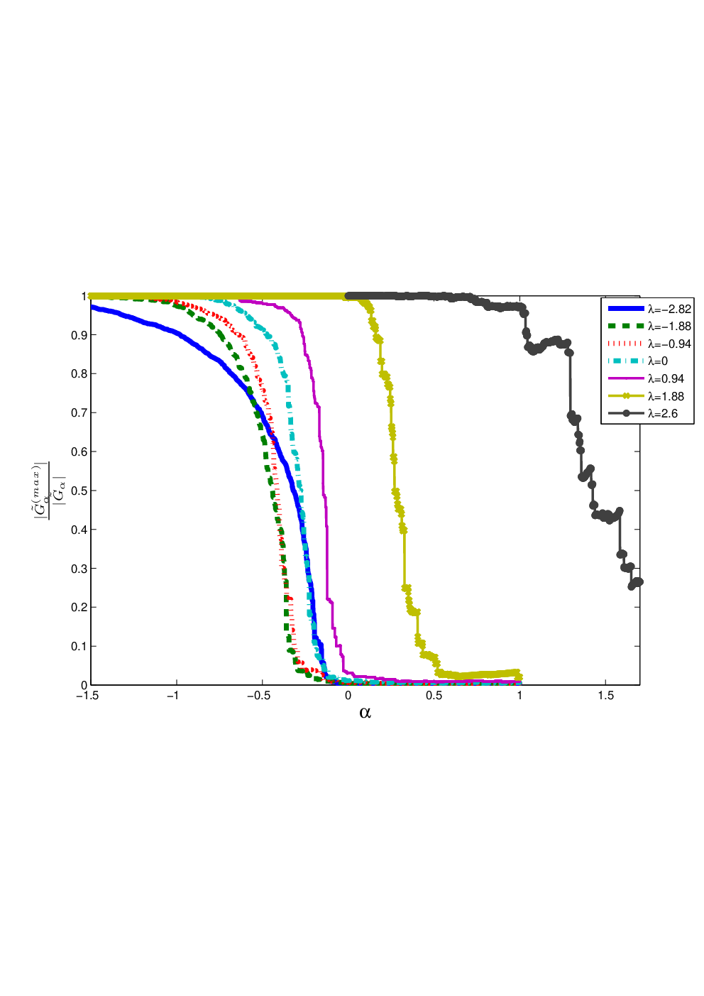
A sharp transition in the normalized size of the level sets is evident: for every value of $\lambda$ there is a narrow window in the vicinity of some $\alpha_{c}(\lambda,d)$, so that for $\alpha>\alpha_{c}$, the ratio $|\tilde{G}_{\alpha}^{(max)}|/|\tilde{G}_{\alpha}|$ is close to zero, while for $\alpha<\alpha_{c}$, $|\tilde{G}_{\alpha}^{(max)}|/|\tilde{G}_{\alpha}|$ is of order one. The described phenomenon was observed for all the tested values of $d$ and for all the examined eigenvectors.
Moreover, repeating the experiment, while varying the size of the graph, we have observed that the value of $\alpha_{c}(\lambda,d)$ does not vary with $n$, while the transition becomes sharper as $n$ increase.

As an example, in figure 2 we plot the variation in $|\tilde{G}_{\alpha}^{(max)}|/|\tilde{G}_{\alpha}|$ for the eigenvectors which correspond to $\lambda\approx 0$, for different realizations of $3$-regular graphs of various sizes.

This extensive corpus of numerical data provides strong evidence supporting the existence of a phase transition for the level sets of $(n,d)$ eigenvectors. Namely, for every $d\geq 3$ and $\lambda\in\sigma(T_{d})$, there may exist an $\alpha_{c}(\lambda,d)\in\mathbb{R}$, so that the level sets of a typical $(n,d)$ eigenvector which corresponds to the eigenvalue $\lambda$ are all microscopic for $\alpha>\alpha_{c}$, while for $\alpha<\alpha_{c}$ a macroscopic component is expected to appear.

Note that the suggested transition differs from the percolation hypothesis for chaotic billiards in two main aspects. First, while for billiards the transition is expected to follow the characteristics of non-correlated percolation, for $(n,d)$ graphs we expect correlations to be relevant (as will be discussed in section 5). Second, Unlike the percolation model for billiards, the critical threshold for regular graphs depends on the corresponding eigenvalue.
In order to estimate the dependence of $\alpha_{c}(\lambda,d)$ on its arguments, we have chosen (somewhat arbitrarily) to identify $\alpha_{c}(\lambda,d)$ with the steepest point of the curve $|\tilde{G}_{\alpha}^{(max)}|/|\tilde{G}_{\alpha}|$, obtained for a graph of size $n=4000$. In figure 3 we present our numerical estimate of the critical curves.

The results suggest that for a given value of $d$, the critical threshold increases monotonically with $\lambda$ for all $d>3$. For the lowest degree, $d=3$, the critical curve $\alpha_{c}(\lambda,d=3)$ shows a minimum in the vicinity of $\lambda\approx-0.52$.
In the next sections we shall show that the numerical resulted summarized above can be reproduced theoretically by considering first the level sets in the random process $\mathcal{GS}_{d}(\lambda)$ on $T_{d}$, and then assuming the validity of the random waves conjecture for the adjacency eigenvectors in $G(n,d)$.

In this section we shall study the distribution of the level sets in $GS$ and prove that they undergo a percolation transition, for which the critical threshold $\alpha_{c}(\lambda,d)$ can be computed.

As the process $\mathcal{GS}_{d}(\lambda)$ is Gaussian and characterized by the covariance operator (2.8), it is possible to rigorously analyze its level sets statistics. Setting

to denote the induced $\alpha$ level sets tree for a given $\psi_{\omega}\in\mathcal{GS}_{d}(\lambda)$, we show that:

As the proof of the theorem is rather technical, we refer the interested reader to [15] where a complete and detailed proof of the theorem can be found. Here, we shall provide the main line of the proof, skipping much of the technical aspects.

It is important to note that for a given $\alpha\in\mathbb{R}$, the $\alpha$-level sets of the process $\mathcal{GS}_{d}(\lambda)$ is a homogeneous vertex process on $T_{d}$. That is, the probability measure of the process is invariant with respect to the symmetries of $T_{d}$.

For any homogenous process, the probability that $v,v^{\prime}\in T_{d}$ belongs to the same connected component depends only on the distance between the vertices and will be denoted by $P_{|v-v^{\prime}|}$. Denoting the sphere of radius $k$ around $v\in T_{d}$ by

we find that the probability that $v$ is connected to its $k$-sphere is at most $|\Lambda_{k}(v)|P_{k}$. Since $|\Lambda_{k}|=d(d-1)^{k}$, we obtain that if

then the probability that the connected component of $v$ exceeds the radius $k$ decays exponentially with $k$, so that the probability to find an infinite component is zero and the process is subcritical.
We should note that the opposite statement is not necessarily correct, i.e. there are percolation processes on $T_{d}$ for which $\liminf_{k\rightarrow\infty}P_{k}^{1/k}>1/(d-1)$, but do not contain infinite components, due to long range correlations.

The influence of the correlations which are induced by the process can be formally evaluated according to the next classification of random processes on trees, introduced in [24].

According to definition 4.2, in a quasi Bernoulli process, the distribution of the process along any simple path is only moderately affected by the realization of the process outside the path. As an example, it can be verified that a Markovian process is quasi Bernoulli.
The quasi Bernoulli classification provides a simple criterion for the relevance of the long range correlations of the process on its macroscopic properties, as suggested by the next lemma [24]¹¹ 1 The theorem as it appears in [24] characterizes general quasi-Bernoulli process on an arbitrary tree graph. For the sake of clarity, we consider here only the restriction of the theorem to invariant percolation processes on $T_{d}$.:

An equivalent phrasing of the lemma is the following: for a quasi Bernoulli process on $T_{d}$, all the components are almost surely finite if their expected cardinality is finite, while if the expected cardinality diverges, infinite components will almost surely exist.
As the $\alpha$-level sets are monotonically decreasing in $\alpha$, we find that in order to prove theorem 4.1 it is enough to show that

• •

  For every $\lambda\in\sigma(T_{d})$ and $\alpha\in\mathbb{R}$, the $\alpha$-level sets of $\mathcal{GS}_{d}(\lambda)$ are quasi Bernoulli

• •

  For small enough values of $\alpha$ there almost surely exist infinite level sets, while for large enough values the $\alpha$-level sets are all finite with probability one.

The first condition guaranties that for every $\lambda\in\sigma(T_{d})$ and $\alpha\in\mathbb{R}$, the probability to find an infinite component is either zero or one (according to lemma 4.3). Assuming the level sets are quasi Bernoulli, and since $\lim_{k\rightarrow\infty}P_{k}^{1/k}(\alpha)$ is monotone in $\alpha$, the second condition ensures that for every $\lambda\in\mathbb{R}$ a supercritical and a subcritical phases exist, where the transition between the two occurs at $\alpha_{c}(\lambda,d)$ which is given by the implicit expression

To verify the existence of a subcritical regime, we note that if a simple path $U$ of length $k$ is contained in an $\alpha$-level set, then necessarily $\forall v_{j}\in U,\psi_{\omega}(v_{j})>\alpha$. Therefore, setting $\Psi_{\omega}(U)=\sum_{j=1}^{k}\psi_{\omega}(v_{j})$, we obtain that

Note that $\Psi_{\omega}(U)$ is a Gaussian random variable, with mean zero and variance

where $\Phi^{(\lambda)}=\phi^{(\lambda)}(0)+2\sum_{j=1}^{\infty}|\phi^{(\lambda)}(j)|$ (2.7).
Since $\phi^{(\lambda)}(j)$ is exponentially decreasing in $j$ (2.7), we find that $\Phi^{(\lambda)}<\infty$. Therefore

where $\beta=(2\Phi^{(\lambda)})^{-1}$.
As $|\Lambda_{k}|=d(d-1)^{k-1}$, we obtain from (4.3) and (4.10) that the $\alpha$-level sets are subcritical for $\alpha>\sqrt{\ln(d-1)/\beta}$.

The existence of infinite $\alpha$-level sets for small enough $\alpha$ is a straight-forward consequence of [25], where it is shown that every homogenous vertex percolation process on $T_{d}$, for which the survival probability exceeds $d/2(d-1)$ is supercritical. As $\psi_{\omega}(v)$ distributes as a normal variable with mean zero and variance one, the vertex survival probability for $T_{\alpha}(\psi_{\omega})$ is given by

Since $d/2(d-1)\leq 3/4$ for every $d\geq 3$ and as according to (4.11) $P_{0}(\alpha)>3/4$ for $\alpha\leq-0.68$, we obtain that for every $d\geq 3$ and $\lambda\in\sigma(T_{d})$, the $\alpha$-level sets of $\mathcal{GS}_{d}(\lambda)$ are supercritical for $\alpha<-0.68$.

In order to prove that the $\alpha$-level sets of $\mathcal{GS}_{d}(\lambda)$ are quasi Bernoulli, we have to show that the long range correlations do not dominate the structure of the random tree $T_{\omega}(\alpha)$ (4.1). A major step toward this goal is the next theorem, which identify the following Markov property of the underlying process $\mathcal{GS}_{d}(\lambda)$:

The proof of theorem 4.4 relies on the observation that for any adjacency eigenvector $\psi:T_{d}\rightarrow\mathbb{R}$, the value of $\psi(v_{1}),\psi(v_{2})$ determines the value of the sum

(see figure 5). Since the distribution of $\mathcal{GS}_{d}(\lambda)$ is invariant with respect to the symmetries of $T_{d}$, we obtain from the last observation that given $\{\psi_{\omega}(v_{j})\}_{j=1}^{k}$, the expected value of $\psi_{\omega}(v_{0})$ is determined by $\psi_{\omega}(v_{1}),\psi_{\omega}(v_{2})$.
Since non-correlated components of a multi-normal random vector are also independent (e.g. [26]), the theorem follows. move a little b$\square$

The described dominance of short range correlations in the process $\mathcal{GS}_{d}(\lambda)$, is utilized in [15], to bound rigorously the effect of long range correlation in $T_{\omega}(\alpha)$, resulting in the identification of $T_{\omega}(\alpha)$ as a quasi Bernoulli process and in the establishment of theorem 4.1.

The last step in the analysis is obtained by solving (4.7) for various values of $d$ and $\lambda\in\sigma(T_{d})$. The results are shown in figure 6, superimposed on the numerical data obtained for $G(n,d)$ graphs and discussed in the previous section (figure 3). The agreement between the $G(n,d)$ data and the critical threshold levels computed for the $\mathcal{GS}_{d}(\lambda)$ process on $T_{d}$ is perfect (including in particular the non monotonic behavior of $\alpha_{c}(\lambda,d=3)$ which is reproduced as well). It strongly supports the random waves conjecture for $G(n,d)$. As was already stated above, the random wave conjecture is valid locally. In the present context, however it applies globally. The proof of the random wave conjecture is still lacking and is a challenge for experts in probabilistic graph theory.

The identification of a phase transition for the level sets of $\mathcal{GS}_{d}(\lambda)$ (and the observed transition for $G(n,d)$ eigenvectors) may be considered as an extension of the percolation hypothesis for random waves on $\mathbb{R}^{2}$ and for chaotic billiards [2]. We would like to conclude this paper by a short comparison between the two models.

We should note that the formal derivation for both of the model is based on the statistical properties of the corresponding random waves model. while the heuristic justification of the percolation hypothesis for two-dimensional random waves is based on arguments which are not clearly justified [27, 28, 29, 12], theorem 4.1 provides a rigorous proof to the existence of a critical level-set for $\mathcal{GS}_{d}(\lambda)$.
In both of the cases, the applicability of the suggested model to the corresponding chaotic system (a billiard or a mixing regular graph) is a consequence of the corresponding random waves model and not of an independent derivation. However the consistency of the models with various numerical tests, such as [9, 2, 30, 11] (for billiards) and [1] (for $(n,d)$ graphs) provide a firm support both for the percolation and the random-waves models.

The arguments behind the two percolation models differ significantly. The percolation hypothesis for two dimensional chaotic billiards is justified in [2, 10] by dimensional arguments which prevents its generalization for generic chaotic systems, or even billiards of higher dimensions. In particular it is based on the topological identification of a random wave with the square lattice [2, 12, 28] and the particular critical threshold $p_{c}=1/2$ for self-dual bond percolation processes on the square lattice. In addition, the neglect of correlation is based on a careful application of the Harris criterion [31], which is valid only for two-dimensional systems [10, 28].

Unfortunately, the identification of a critical level set for the process $\mathcal{GS}_{d}(\lambda)$ demonstrates the same weakness, as it utilizes repeatedly the tree structure of $T_{d}$. Nevertheless, the identification of a critical level sets for the two seemingly non-related waves ensembles hints on a universal mechanism behind the phenomena. In addition the dependence of the critical point (4.7) in the spectral parameter $\lambda$, implies that the suggested transition for the eigenfunctions of a generic chaotic system (assuming it indeed exists) may exhibit a more complicated behavior then the simple model which is suggested in [2].

References

- [1] Y. Elon. Eigenvectors of the discrete Laplacian on regular graphs—a statistical approach. J. Phys. A, 41(43):435203, 17, 2008.
- [2] E. Bogomolny and C. Schmit. Percolation model for nodal domains of chaotic wave functions. Physical Review Letters, 88(11):114102, March 2002.
- [3] D. Jakobson, S. D. Miller, I. Rivin, and Z. Rudnick. Eigenvalue spacings for regular graphs. arXiv:hep-th/0310002v1, September 2003.
- [4] I. Oren, U. Smilansky, and A. Godel. Trace formulae and spectral statistics for discrete laplacians on regular graphs (i). J. Phys A., 42:415101, 2009.
- [5] I. Oren and U. Smilansky. Trace formulae and spectral statistics for discrete laplacians on regular graphs (ii). J. Phys A., 43:225205, 2010.
- [6] A. Broder and Shamir E. On the second eigenvalue of random regular graphs. Foundations of Computer Science, Annual IEEE Symposium on, 0:286–294, 1987.
- [7] J. Friedman. A proof of Alon’s second eigenvalue conjecture and related problems. Mem. Amer. Math. Soc., 195(910):viii+100, 2008.
- [8] R. M. Stratt, N. C. Handy, and W. H. Miller. On the quantum mechanical implications of clasical ergodicity. Jour. of Chem. Phys., 71:3311–3322, October 1979.
- [9] G. Blum, S. Gnutzmann, and U. Smilansky. Nodal domains statistics: A criterion for quantum chaos. Physical Review Letters, 88(11):114101, March 2002.
- [10] E. Bogomolny and C. Schmit. Random wavefunctions and percolation. Journal of Physics A Mathematical General, 40:14033–14043, November 2007.
- [11] E. Bogomolny, R. Dubertrand, and C. Schmit. SLE description of the nodal lines of random wavefunctions. Journal of Physics A: Mathematical and Theoretical, 40(3):381, 2007.
- [12] J. P. Keating, J. Marklof, and I. G. Williams. Nodal domain statistics for quantum maps, percolation, and stochastic loewner evolution. Physical Review Letters, 97(3):034101, 2006.
- [13] D. Stauffer and A. Aharony. Introduction to percolation theory, 2nd edition. Taylor & Francis Ltd., London, 1994.
- [14] N. Alon, I. Benjamini, and A. Stacey. Percolation on finite graphs and isoperimetric inequalities. Ann. Probab., 32(3A):1727–1745, 2004.
- [15] Y. Elon. Gaussian waves on the regular tree. arXiv:0907.5065v2 [math-ph], September 2009.
- [16] S. Hoory, N. Linial, and A. Wigderson. Expander graphs and their applications. Bull. Amer. Math. Soc. (N.S.), 43(4):439–561 (electronic), 2006.
- [17] N. C. Wormald. The asymptotic distribution of short cycles in random regular graphs. J. Combin. Theory Ser. B, 31(2):168–182, 1981.
- [18] B. Bollobás and W. F. De la Vega. The diameter of random regular graphs. Combinatorica, 2(2):125–134, June 1982.
- [19] P. Cartier. Fonctions harmoniques sur un arbre. In Symposia Mathematica, Vol. IX, pages 203–270. Academic Press, London, 1972.
- [20] B. D. McKay. The expected eigenvalue distribution of a large regular graph. Linear Algebra Appl., 40:203–216, 1981.
- [21] R. Brooks. The spectral geometry of -regular graphs. J. Anal. Math., 57:120–151, 1991.
- [22] M. V. Berry. Regular and irregular semiclassical wave functions. Journal of Physics A Mathematical General, 10:2083–2091, 1977.
- [23] A. Steger and N. C. Wormald. Generating random regular graphs quickly. Combin. Probab. Comput., 8(4):377–396, 1999. Random graphs and combinatorial structures (Oberwolfach, 1997).
- [24] R. Lyons. The Ising model and percolation on trees and tree-like graphs. Comm. Math. Phys., 125(2):337–353, 1989.
- [25] O. Häggström. Infinite clusters in dependent automorphism invariant percolation on trees. Ann. Probab., 25(3):1423–1436, 1997.
- [26] I. A. Ibragimov and Y. A. Rozanov. Gaussian random processes, volume 9 of Applications of Mathematics. Springer-Verlag, New York, 1978. Translated from the Russian by A. B. Aries.
- [27] G. Foltin, S. Gnutzmann, and U. Smilansky. The morphology of nodal lines random waves versus percolation. Journal of Physics A Mathematical General, 37:11363–11371, November 2004.
- [28] G. Foltin. The distribution of extremal points of Gaussian scalar fields. J. Phys. A, 36(16):4561–4580, 2003.
- [29] A. Aronovitch and U. Smilansky. The statistics of the points where nodal lines intersect a reference curve. J. Phys. A, 40(32):9743–9770, 2007.
- [30] Y. Elon, S. Gnutzmann, C. Joas, and U. Smilansky. Geometric characterization of nodal domains: the area-to-perimeter ratio. J. Phys. A, 40(11):2689–2707, 2007.
- [31] A. B. Harris. Effect of random defects on the critical behaviour of ising models. Journal of Physics C: Solid State Physics, 7(9):1671–1692, 1974.