Black hole lasers in Bose–Einstein condensates
Abstract
We consider elongated condensates that cross twice the speed of sound.
In the absence of periodic boundary conditions, the phonon spectrum possesses a discrete and finite set of complex frequency modes that induce a laser effect. This effect constitutes a dynamical instability and is due to the fact that the supersonic region acts as a resonant cavity.
We numerically compute the complex frequencies and density–density correlation function. We obtain patterns with very specific signatures.
In terms of the gravitational analogy, the flows we consider correspond to a pair of black hole and white hole horizons, and the laser effect can be conceived as a self-amplified Hawking radiation. This is verified by comparing the outgoing flux at early time with the standard black hole radiation.
Online supplementary data available from stacks.iop.org/NJP/12/095015/mmedia
Accepted: 11 Jun 2010.
http://stacks.iop.org/1367-2630/12/095015
Contents
1 Introduction
In 1981, Unruh suggested [1] that the analogue of black hole radiation could be observed in a quantum fluid that crosses the speed of sound, thereby forming a sonic horizon. Since then, several types of fluids and several types of flows were considered [2]. Very recently, a near-stationary supersonic flow engendering a pair of horizons (a black hole one followed by a white hole one) was realized in a Bose–Einstein condensate [3]. In such a background, because of the anomalous dispersion of Bogoliubov phonons, one expects to get a kind of laser effect [4]–[6] due to a self-amplification of the Hawking radiation.
The first aim of this paper is to provide the theoretical basis of this effect starting from the Bogoliubov–de Gennes equation, i.e. without making use of the gravitational analogy. In this we apply to flows containing two horizons the treatment of [7] that was only applied to a single (black hole or white hole) sonic horizon. Following [6] we then establish that the laser effect is governed by a discrete set of complex frequency modes that correspond to the resonant modes of the cavity formed by the region bordered by the two horizons. In a classical description, this discrete set governs the dynamical instability of the flow. The second aim is to compute the spectrum of the complex frequency modes by theoretical and numerical methods. The excellent agreement of the results validates both the concepts and the semi-classical methods used in the theoretical approach. Finally we consider two observables: the mean number of emitted phonons, and the two-point function of the phonon field that governs the density–density correlation pattern [8, 9]. At sufficiently late time, both observables are governed by a single mode, the most unstable one. In this late time regime, their behaviours are identical to those one would obtain using a classical description of the density perturbations. At early time instead, when starting from vacuum configurations, correspondence with the quantum phonon flux emitted by a black hole horizon [7] is established.
The propagation of phonons in flows containing two horizons has already been considered. However, toroidal configurations with periodic boundary conditions were generally used [10, 11]. In that case, the spectrum is very complicated because it results from a combination of two effects: the discreteness of the wave vectors defined on the torus interferes with that associated with modes that are trapped in the supersonic region. As a result, not only the analysis is difficult, but the relationships with the Hawking effect and the black hole laser effect [4]–[6] are hard to draw. On the contrary, when dealing with continuous wave vectors, the analysis of the complex frequency mode is simpler, and the relationship with Hawking radiation is easily made.
We have organized this paper as follows. In section 2 we present the Bogoliubov–de Gennes equation in a way that is suitable for our aims. In section 3 we determine the spectrum of asymptotically bound modes, and explain why complex frequency modes appear when the speed of sound is twice crossed. We then compute the eigen–frequencies using semi-classical methods. In section 4 we numerically solve the Bogoliubov–de Gennes equation and compute the spectrum. We then evaluate the mean occupation number and compare it with the spectrum one would obtain if only the black hole horizon were present. We finally evaluate the correlation pattern of the density–density two-point function.
2 Framework
2.1 Black-hole–white-hole geometries
Using the analogy [1, 2] between the wave equation governing sound propagation in a moving fluid and that governing light propagation in a curved space-time, one can associate an acoustic geometry to the fluid flow. In 1+1 dimensions, these geometries are of the form [4]
| (1) |
where is the flow velocity and the speed of sound. In this language, a black-hole–white-hole geometry is obtained when crosses twice . Indeed, a sonic horizon is present whenever crosses . Assuming that the fluid flows from right to left (), the location of a horizon is given by . In our case, we set the location of the white hole horizon and that of the black hole respectively to and . These divide the -axis in three regions, which we call I on the left of the white horizon (), II between the two horizons () and III on the right of the black horizon (). The flow is supersonic in the internal region II and subsonic otherwise. The opposite case where the velocity is subsonic inside does not give rise to a laser effect, and will be considered elsewhere.
In the present work, our analysis is restricted to the following stationary profiles:
| (2) |
which generalize to two horizons those used in [7]. is the sound speed at the horizons, is the distance between them, determines the size of the near-horizon regions where the metric is not flat, controls the sharpness of the transition to the flat regions, and and control the surface gravities. Indeed, the surface gravity is defined by [2]
| (3) |
which yields for the white hole and for the black hole. The metric (1) is then completely fixed by introducing an extra parameter :
which specifies how is shared between and . When restricting to the cases where
| (7) |
the range of and is limited. The allowed values are graphically illustrated by the shaded area in figure 1, left panel. Three velocity profiles corresponding to different couples are plotted in figure 1, right panel.

2.2 Density perturbations in Bose Einstein condensates
We present the main steps leading to the equations for linear density perturbations in Bose–Einstein condensates [12], having in mind cases where the condensate crosses the speed of sound. We follow [7], where more details can be found.
At low temperature, the quantum properties of a gas of weakly interacting atoms are efficiently described by a second quantized field satisfying the commutation relation
| (8) |
and by its Hamiltonian
| (9) |
where is the atom mass, the external potential and the effective coupling. The last two quantities can depend on both and . When a significant fraction of the atoms condense, it is meaningful to expand in a -number function , describing the condensed part, plus a field operator , describing (relative) density perturbations over the condensate
| (10) |
In what follows, we consider elongated condensates, which means that the transverse excitations have sufficiently high energies that they are not excited. In this case, and are effectively one-dimensional fields. For simplicity, we also assume that the condensate is infinitely long, in order to avoid discussing the discreteness of the longitudinal wave number . The discrete case is indeed more complicated, and treated in details in [11]. Finally, we assume that the condensate is stationary, which means that is of the form
| (11) |
where is the chemical potential, the mean density of condensed atoms and
| (12) |
is their mean velocity. In this case, the Gross–Pitaevskii equation
| (13) |
reduces to
| (14) |
where the second equation is the continuity equation for a stationary flow.
At the linear level, obeys the Bogoliubov-de Gennes equation. In the present case, using (10) and (14), this equation reads
| (15) |
where we introduced the -dependent speed of sound
| (16) |
and where
| (17) |
reduces to the usual kinetic operator when the background condensate is homogeneous. The second expression is only valid in stationary flows. Equation (15) tells us that the perturbation is coupled to the condensate only through the functions and . The disappearance, from (15), of the potential , the quantum potential , and the coupling constitutes an essential step towards the notion of the acoustic metric of (1); see [7] for more details.
3 Theoretical analysis
3.1 Spectrum of bound modes and quantization
In stationary condensates, the spectrum of (20) can be characterized using very general properties. These are first, the fact that the eigenmodes are asymptotically bound (to guarantee that they have a well-defined norm since the spatial domain of is infinite), second, the Hermiticity of (20), i.e. its self-adjointness with respect to the scalar product defining the eigen-modes norm, and third, that this scalar product is not positive definite, as it is the case here, see (93), and for bosonic fields, see e.g. [13].
When these conditions are met, the spectrum of (20) contains a continuous set of real frequency modes labelled by and a discrete index , plus, possibly, a discrete and finite set of complex frequency modes that appear in pairs with complex conjugated frequencies. (If the scalar product were positive definite, as is the case for fermions, the spectrum of (20) would be purely real.) Throughout this paper, complex frequencies shall be written as , where is a positive integer which labels the discrete set of pairs, and where and are both real and positive. The other cases are reached by complex conjugation and/or multiplication by . The discrete index describes the subset of modes with the same real frequency. As explained below, in one dimension, it contains two or four modes depending on whether the flow is subsonic or supersonic.
As a result, when propagating in a stationary condensate, , obeying (18) and (19), can always be expanded (see appendix B) as
| (21) |
where the modes satisfy the normalization relations
| (22) | |||
| (23) |
Correspondingly, the operators , , satisfy the commutation relations
| (24) | |||
| (25) |
All the other scalar products, and all other commutators, vanish. In particular, one has . Hence and are not destruction operators. In fact, the operators and form pairs [6] that characterize complex, i.e. with two degrees of freedom, harmonic oscillators that are unstable, and for which therefore there is no notion of quanta. (Concomitantly, one verifies that the norm vanishes.) It should be noticed that the eigenfrequencies associated with and are complex conjugated from each other (respectively and ), something guaranteed by the Hermiticity of (20).
In terms of the above eigenmodes and operators, (20) reads
| (26) |
The first line contains the usual sum over harmonic oscillators of real frequency and the -number term accounting for the depletion, while the second line is due to the complex frequency modes. It should be noticed that the unusual form of the second -number term follows from the unusual scalar product of (23). This Hamiltonian is not bounded from below due to the terms. Hence the vacuum can no longer be defined as the ground state of , as one might have expected since one is dealing with unstable oscillators. This gives rise to some ambiguity when choosing the initial ‘vacuum’ state (see section 3.4).
Eqs. (21) and (26) can be rewritten in a more familiar form by decomposing each couple () into two couples of destruction/creation operators , and , , as shown in appendix B. The field becomes
| (27) |
and the Hamiltonian (26)
| (28) | |||||
We conclude with two remarks. Firstly, if one can describe the discrete set using the operators, there is a price to pay as the associated modes , , , are not frequency eigenmodes. Hence their time dependence cannot be factorized. Secondly, in usual circumstances, the discrete set of complex frequency modes is empty, as is the case in homogeneous and in near-homogeneous condensates. Nevertheless, when the condensate crosses twice the speed of sound, the discrete set is (generally) nonempty. To explain why, we first need to study the spectrum in homogeneous subsonic and supersonic flows, and then understand how to paste the corresponding modes when the flow crosses the speed of sound. When solving this, the dispersive properties of become essential, as we now recall, and as first understood in [4].
3.2 Mode analysis
Inserting the field expansion (21) in (15), one obtains a system of two -number equations
| (29) |
The couple can be formed by either the real frequency modes , or the complex frequency modes or and, accordingly, can be real or complex. Eliminating from the above system, one obtains [7]
| (30) |
When the background quantities are independent of , Fourier modes are solutions of (30), provided is a (possibly complex) root of the dispersion relation
| (31) |
where is the frequency in the comoving frame, and where is a typical value of the sound speed, we take to be that at the horizons, see section 2.1. We also introduced
| (32) |
which gives the characteristic dispersive scale. When sending , (31) becomes the relativistic equation since the quartic term drops out. Similarly, (30) becomes the Euler equation governing sound waves. Instead, when keeping this term, the dispersion relation (31) possesses four roots, some of which can be complex. As we shall progressively see, the two extra roots are at the origin of the laser effect.
3.2.1 Modes in homogeneous condensates.
In subsonic flows, , for real , two roots are real, and describe the right and left moving solutions. The other two are complex, conjugated to each other, and correspond to modes that are asymptotically growing or decaying, say to left. Only the first two should be used in (21), as the last two are not asymptotically bound.
In supersonic flows, the situation is quite different. For real , there exists a critical frequency such that the four roots of (31) are [7]
- •
: all real;
- •
: two real and two complex ones, as in subsonic flows.
See figure 2 for a graphical solution of the dispersion relation (31).

When is real, the normalization of the (bound) modes can be easily worked out, as it is, up to a trivial factor, independent of the constant velocity (because of Galilean invariance). Let us write
| (33) |
where spans over four values if and and over two values elsewhere. Using the mode normalization (22)
| (34) |
from the mode equation (29) and the dispersion relation, one has
| (35) |
where
| (36) |
is independent of . Equations (34) and (35) fix and except for a common phase. Taking both and real, one obtains
| (37) |
In supersonic flows, when , the two modes associated with the extra real roots of (31) have negative norm. However, for , the corresponding modes have a positive norm. So, the field is expanded as11 1 In terms of the doublets defined in appendix B one has (38)
| (39) | |||||
where is the Heaviside function.
In subsonic flows one obtains the same expression, but without the last term in each bracket since the extra real roots are absent.
3.2.2 Modes in black-hole–white-hole geometries.
To obtain the spectrum in condensates that cross twice the speed of sound, i.e. in flows defining the geometry of (2), we need to take into account the nontrivial propagation in the non-homogeneous regions localized near the two horizons, and the fact that each subsonic region is now defined on the half line and no longer on the full real axis. Then, we need to identify the number of globally defined independent modes.
It should be noted that this set does not depend on the particular form of the mode equation, but mainly resides on the behaviour in the internal region II and in the asymptotic flat external regions I and III described in section 2.1. Therefore, the result is the same when studying a phonon field in a BEC, as in the present paper, or a generic scalar field with superluminal dispersion relation as in [6]. As explained in this reference, in geometries described by (2), there is a continuous double set (right-going and left-going waves) of real frequency modes, and the discrete set of complex frequency modes is generally not empty. Here we give a more mathematical argument yielding the same result.
In flows (2), two asymptotically flat and subsonic regions play the most important role in defining the set of modes, for both real and complex. For real, there are three bounded modes: the two usual propagating modes associated with the real roots of (31) plus the mode that asymptotically decays. This mode should now be taken into account as it is bound in the subsonic region where it is defined. We will call the two sets of three modes and , respectively for the left (I) and right (III) asymptotic region, where the superscript takes three values: to characterize the asymptotic right-going -mode, the left-going -mode and the decaying -mode, named after the paper of Corley and Jacobson [14]. In the internal region II, we have four modes that we call with . Since this region is bound, the four roots of (31) should be taken into account.
Therefore, any globally defined solution of frequency can be expanded in two forms by referring to its left, or right, asymptotic behaviour:
| (40) |
Moreover, each partial wave or can be written in term of the :
| (41) |
Putting together the above equations, one obtains
| (42) |
This system of four equations in six unknowns (the coefficients and ) has a two-dimensional set of solutions, corresponding to two linearly independent modes. For instance, one can choose as independent solutions, and , the two right-going and left-going in-modes, defined as the solution of (42) with respectively and . Similarly, one can chose the out-modes and defined respectively by and . Using the scalar product of (22) to normalize these modes, the two sets are related by [6]
Unitarity imposes , and .
Let us now move to the complex frequency case. Because all expressions are analytic in , the above analysis applies as such when replacing by . The novel aspects only come through the condition that the modes be asymptotically bound. Indeed, implies that , the asymptotic wave number of the real root of (31) (more precisely of its analytical continuation in ), acquires a positive imaginary part. Thus the mode diverges at , unless one puts . Similarly, on the right side, the mode diverges at , and imposing that it is bound requires . However, these two conditions imply that the system (42) has only the trivial solution , except when its determinant vanishes. This condition defines an equation for the complex frequency that has a finite set of solutions: .
3.3 The semi-classical treatment of [6]
Having established the condition that defines the complex frequencies , we now turn to the question of calculating them. Since the above algebraic method does not depend on the specific form of the mode equation, the semi-classical treatment of [6] applies to the present case. Therefore, we just summarize the results without going into the details. One should nevertheless pay attention to the fact that one is dealing with modes doublets and to the normalization of these modes.
When the background is not homogeneous but varies slowly with respect to the wavelength of the perturbation, the exact solutions are well approximated by their WKB approximation, which can be directly inferred from (37)
| (46) |
The -dependent wave numbers are real roots of the dispersion relation (31) in a stationary inhomogeneous flow characterized by and :
| (47) |
Ignoring the quartic term, one obtains the dispersion relation of a massless field propagating in the acoustic metric (1). Equations are valid in the three regions I, II, III but not close to the horizons where the gradients of and cannot be neglected.
The theoretical analysis can then be greatly simplified when taking into account the fact that the mixing between and modes is usually negligible [7, 15]. (However the numerical analysis of the next section does not rely on this simplifying assumption.) In this approximation, the laser effect is completely due to the -modes (for flows to the left ). Considering the in-mode in the internal region II, it can be written as a superposition of three WKB waves:
| (48) |
where are the two negative frequency -modes, corresponding to the two extra roots , being the most negative one, see figure 2.
In [16] it was shown that the propagation from one horizon to the other is efficiently described by a unitary scattering of a two-component vector, whose first component represents the -wave and the other represents the trapped wave, described either by or . The matrix is decomposed in four elementary matrices
| (49) |
representing (from 1 to 4) the scattering at the white hole horizon, the propagation between the white and the black hole horizon of and , the scattering at the black hole horizon and the propagation back to the white hole horizon of . These matrices are
| (50) |
where
| (51) |
are the Hamilton–Jacobi actions governing the phase of the WKB modes, and and are the two turning points. Moreover, by unitarity, the parameters in and must satisfy , , .
For real frequency modes, the condition that the trapped mode be single valued imposes [6]
| (52) |
where is real by unitarity. From this matricial equation, one obtains
| (53) |
and therefore the coefficients of (48) are
| (54) |
For complex frequency with , imposing that the incoming branch vanishes, one obtains
| (55) |
which implies
| (56) |
Equations (53), (54) and (56) are the central equations we shall use to analyse the results of the numerical integration. Even though these equations have been obtained through a semi-classical reasoning, their validity goes beyond that of the WKB approximation, as shall be established by the remarkable agreement between the relations one can derive from them and the numerical results.
The main prediction concerns the relation between , solutions of (56), and the behaviour of the coefficients of (54). Indeed, solution of , is a pole of . Therefore, when is small enough (this is always true in our numerical situations), the pole is close to the real axis and the behaviour of for real frequencies is dominated by the contribution of the pole:
| (57) |
from which
| (58) |
Thus, should be well described by a sum of Lorentzians characterized by the complex frequencies . In figure 3 we plot obtained from numerical simulations and the corresponding fitted sum of Lorentzians. The agreement is excellent.


We conclude this analysis by showing that a semi-classical treatment furnishes approximate expressions for the complex frequencies . Assuming , and are much smaller than 1, one can expand the condition in powers of these quantities. To zeroth order, one has real, with solution of the Bohr–Sommerfeld condition [6]
| (59) |
where . A semi-classical treatment gives . A more refined estimate [17] gives
| (60) |
where is Euler’s Gamma function.
To first order in , , and , gives
| (61) | |||
| (62) | |||
| (63) | |||
| (64) |
where is the time for the trapped mode to make a full bounce. The phase modulates the frequency imaginary part and the first order correction to its real part , as shall be seen in section 4.2.2.
3.4 Observables: Phonon fluxes and density–density correlation patterns
Having identified the set of eigenmodes, we now consider observable quantities. We shall study both the phonon flux emitted by the black-hole–white-hole system, and the non-local density–density correlation pattern, as they illustrate very different aspects of the laser effect.
In what follows, we work in quantum settings because we shall assume that the state at the formation of the supersonic region is vacuum. In classical settings, the dynamical instability (the laser effect) would be present only if the initial density-perturbation possesses a non-vanishing overlap with some complex frequency mode, see section V.A. in [6]. For a perfectly adiabatic formation of the supersonic flow, the amplitudes associated with these modes would be zero. However, any small deviation from adiabaticity will trigger the instability, thereby engendering a behaviour very similar to that derived in quantum settings. In fact, as we shall see, the main difference between the quantum and the classical treatment is at early times because in the quantum vacuum all complex frequency modes contribute to the observables through the spontaneous excitation.
To compute observables, we first need to choose the quantum state. Because of the instability, the energy (26) is unbounded from below, and there is no clear definition of the vacuum. Nevertheless, if the formation of the supersonic region at time is adiabatic, and if the temperature condensate is low enough, i.e. much smaller than , the Heisenberg state of the system can be approximated by the state annihilated, at that initial time, by the destruction operators , , of (27).22 2 We applied the standard reasoning to both the and the operators because , the imaginary part of the complex frequency , is smaller than a tenth of . Since the operators , are not stationary, the expectation values will not be stationary either, and will instead depend on the lapse of time since the formation at . In what follows all expectation values will be computed in this state.
The two observables we shall study are related to the density fluctuation . Given the definition of in (10), is given by
| (65) |
where is Hermitian. Its expansion in terms of operators is
| (66) |
where
| (67) |
In the vacuum defined at , the two-point function is
| (68) | |||||
Because of the complex frequency modes, it is not a function of only. This differs from the cases of a single black hole (or white hole) horizon, where the two-point function is stationary in vacuum [7].
To extract more physical information, it is convenient to return to the frequency eigenmodes appearing in (21). Defining
| (69) |
the two-point function becomes
| (70) |
The first line gives the (vacuum) contribution of the real frequency modes. Since these are only elastically scattered, see (3.2.2), they stay in their ground state and contribute neither to the emitted fluxes nor to the pattern of density–density correlations. The third line contains a mixed contribution of the growing and decaying modes . It does not contribute to the fluxes at any time because vanishes in region I, and does it in III, see the paragraph after (3.2.2). Moreover, since it only depends on , it does not significantly contribute to the correlation pattern at late time. Therefore, both fluxes and correlation patterns are governed by the growing mode contribution, the first term of the second line in .
It is clear that at late times, i.e. , all observables are dominated by the mode with the largest . For instance, the equal time density–density correlation function is asymptotically given by
| (71) |
The real part of the frequency drops out and, as a result, the locus of the maxima does not propagate with time. This function is studied for various modes in section 4.4. In case the initial state is not vacuum but a thermal state, the above two-point function would be multiplied by , where is the mean occupation number, which depends in a nontrivial way both on the temperature and on the blue shift effect due to the horizons (see equation (46) in [7]). Similar considerations apply to the quantity that is considered below. Had we worked in classical settings, we would have obtained a coherent wave whose behaviour in and is the same as that of at fixed , see equation (54) in [6]. The main difference arises from the fact that the classical wave amplitude is fixed by initial conditions.
It is also interesting to study the onset of the instability for earlier time, i.e. . To this end, we consider the following quantity:
| (72) | |||||
It governs the probability that a density fluctuation of frequency be observed during the interval at some fixed location in the subsonic region III, see [6].
When , when the discrete set labeled becomes continuous, and when is sufficiently large, behaves as in the Golden Rule: , i.e. the lapse of time times , the mean occupation number of frequency . There can be pre-factors that depend on the strength of the coupling, the amplitude of the mode at , if one deals with a derivative coupling.
It is more interesting to study as a function of for a given black-hole–white-hole geometry, and to compare it with , the corresponding quantity computed in the case where only the black hole horizon would be present. When , the two observables behave in a very similar manner, even when only a few (say 10) complex frequency modes exist in the black-hole–white-hole case. This shall be seen by a numerical analysis in section 4.3, but can be also understood from the properties of the growing modes , see the central paragraph of section V.B.5 in [6].
For classical settings, the laser effect is present only when the initial density-perturbation profile is characterized by a non-vanishing amplitude of some complex frequency mode. Since for adiabatic formation of the horizons all the amplitudes associated with those modes are zero, no laser effect appears in this case. However, even a small deviation from perfect adiabaticity causes the presence of instabilities. The main difference in the quantum framework is therefore the possibility to make the system unstable through the spontaneous excitation of complex frequency modes.
4 Numerical results
4.1 The method
In a few words, we describe how we proceeded to solve numerically (29) in the flows described by (2) and (2.1). As in the case of a single black hole or white hole horizon, when working with a fixed frequency, the main task is to avoid the growing mode contaminating the oscillatory modes. The way to get rid of this difficulty is by integrating from the subsonic region towards the horizon into the supersonic region where there is no growing mode [14].
Basically we solved separately the mode equation from region I to region II, and from region III to region II, using a code adapted from [7]. In each case, as in that reference, we integrated the equations for initial conditions describing the three acceptable modes in regions I and III: the right-moving -mode, the left-moving -mode and the decaying mode. Then for each of them we computed the amplitudes of the four oscillatory modes in the supersonic region II. The two globally defined modes are built using the procedure described in section 3.2.2. To obtain the scattering from I to III, we eliminated the amplitudes in region II.
4.2 The discrete set of complex frequencies
Two strategies can be used to determine the complex frequencies , solutions of (56). They can be obtained either by solving directly the linear system (42), or by determining the center and the width of the Lorentzians in of (58). We use the latter to localize them and the former to refine the results and study how they depend on the various parameters of the system.
To give a first idea, in figure 3 we represent as a function of (green points) for two different values of , the distance between the horizons. A sum of Lorentzians functions (red line) is fitted to the data obtained from the numerical analysis (see (58)). The quality of the fit confirms the correctness of the theoretical analysis of section 3.3 and of [6]. In the following sections, we study the dependence of on both the parameters describing the geometry (see the velocity profile (2)) and the dispersive scale of (31). The dependence on is not reported here, since it induces no significant change.33 3 The role of of (2) is to govern the smoothness of the transition from the near-horizon region to the flat asymptotic ones. A smaller corresponds to smoother transition, while a larger corresponds to steeper transition and, consequently, to a larger almost-flat region between the horizons. The usefulness of is essentially technical: it allows one to control the numerical analysis when , the distance between the horizons, is comparable to , the width of the transition between regions I–III of section 2.1. Before proceeding we make some comment about the properties and the validity of the Bohr–Sommerfeld condition (59).
4.2.1 The validity of the semi-classical approximation.
The action appearing in (59) contains the difference of two wave vectors: . These have the same sign (negative for positive ), as they belong to the same -branch of the dispersion relation (see figure 2), but they have opposite group velocity: describes a right-going mode with respect to the lab, whereas a left-moving one. This peculiarity give rise to an unusual phenomenon. In the usual case, eigenmodes with small (large) frequency correspond to small (large) Bohr–Sommerfeld numbers , i.e to modes with few (many) nodes. In the present case instead, a large corresponds to low frequency modes and vice versa. This can be understood from (59). Because the wave vectors appeared subtracted, a small implies close to and this happens for close to (see figure 2). On the contrary, a large implies a large difference between and , that is, close to 0.
This has an unusual consequence. The Bohr–Sommerfeld condition is more reliable when the action is large, that is for . In the present case this happens for small . On the other hand the WKB approximation is expected to fail for small , as can be verified by the fact that of (60) cannot be neglected when . Both these expectations are confirmed in figure 4 where we compare the numerical results with the predictions obtained with the standard WKB approximation (green lines) and with the improved method (red lines), that is when using (60). Firstly, the agreement between the Bohr–Sommerfeld condition and the numerical results is worse for close to and gets better when increases. Secondly, at low frequency, while the quality of the standard WKB prediction (green lines) becomes worse, the improved method continues to work very well, thereby establishing its validity. Further studies about the agreement of the improved method and numerical results are in preparation [17].

4.2.2 The birth of modes as a function of the distance between the horizons.
In figure 5, left panel, we plot for the entire spectrum of complex frequency modes as a function of the half-distance between the horizons , all other quantities being fixed. On the right panel, is plotted as a function of , for =4 and for the same values of the other parameters.

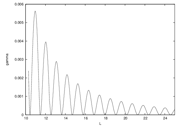
As conjectured in [6], when grows, all values increase, and when there is enough ‘room’, a new eigenmode appears with . As a result, the eigenfrequencies become denser close to , because they neither cross it nor disappear.
It is interesting to consider more closely the birth of new modes near . A rather difficult question to answer is the following: when extra mode appear, does the imaginary part of the frequency vanish, as found in figure 1 of [18], or not? This question is physically relevant in that it governs the continuous character of the stability of the system: if vanishes, it implies that the birth of new modes leads to a continuous behaviour in (as one can expect on the general ground that the properties of the eigenmodes, solutions of (15), continuously depend on the parameters appearing in that equation). From figure 5, which is based on the roots of the determinant in (42), no definite conclusion can be drawn since there is a loss of numerical precision for . A more reliable method consists in studying the behaviour of on the real frequency axis. We created a gif-animation (eigenfrequencies.gif (available from stacks.iop.org/NJP/12/095015/mmedia)) of as a function of for increasing values of to illustrate the appearance of the new eigenfrequencies. From this it is quite clear that when a new eigenmode appears, both the real part and the imaginary part of vanish, as was also found in the appendix of [19].
Another important feature confirming the theoretical analysis of section 3.3 is the presence of superposed oscillations on the overall trend of . In fact, the latter is given by the solution of the Bohr–Sommerfeld equation (59), whereas the oscillations are due to the deviations governed by the sine in of (62). For the imaginary part instead, there is no zeroth-order contribution, and the dominant contribution to the right plot of figure 5 is given in (61).
4.2.3 Asymmetric velocity profiles.
Using asymmetric velocity profiles, namely different surface gravities and , does not lead to substantial modifications of the spectrum. The only observable change concerns . When , vanishes for some particular combination of parameters, as can be seen in figure 5, right panel. Equation (61) can indeed be rewritten as
| (73) |
which shows that when , vanishes when the cosine does, and this is because the scatterings at the black and the white horizons destructively interfere with each other. When the two surface gravities are different, is non-zero and can no longer vanish (see figure 6).

The non-zero offset is significant only for sufficiently large values of , which requires that be large enough, since all . Using the standard expressions and , which furnish reliable estimates [7], the ratio between the offset and the amplitude of the oscillation is
| (74) |
Even though this function increases in when , the consequences of this are never important because when the ratio is large, the corresponding mode will not significantly contribute to the instability since , as can be seen from (73).
4.2.4 The – mixing and the parameter .
The mixing between the -modes, which are right-going in the lab in subsonic flows, and the -modes is controlled by the transmission coefficient of (3.2.2). In figure 7, is plotted as a function of for a fixed frequency . The transmission coefficient is almost 1 between and . Thus, for values of in this range the – mixing is negligible, as was noticed in [7] for a single black (or white) hole. In this regime the approximation discussed in section 3.3 is valid. There is, however, an important difference with respect to the single black hole case. In black-hole–white-hole geometries, the transmission coefficient deviates from zero when approaching a resonance. When working with a fixed , we found two sharp spikes figure 7 for and which exactly correspond to two unstable modes. Moreover, the width of the spikes is almost equal to the corresponding . We also looked for complex eigenfrequency associated with the other two local and broad minima of , at and , and we found two eigenmodes with respectively and , i.e. in the neighbourhood of the chosen frequency . These considerations show that close to resonances one cannot completely neglect the – mixing. Nevertheless, as shown in figure 4, the improved treatment of the Bohr–Sommerfeld equation produces very good estimates for the values of the real part of the complex frequencies.

4.2.5 The role of the maximal frequency .
In [7, 15], it was shown that the deviations, due to dispersion and w.r.t. the standard Planckian distribution, of the spectrum emitted by a single BH, or WH, are mainly governed by . However, the latter depends both on the UV scale and the velocity profile (see section 3.2.2). The relationship takes the form
| (75) |
Hence the same value of can be reached from very different cases, and yet it was found that the fluxes are hardly sensitive to this. In the present case however, this insensitivity is lost because the number of resonances directly depends on . This can be understood by studying (59), and is manifest in figure 8, where is plotted as a function of for two different values of .

4.3 Growth of the asymptotic phonon fluxes


In figure 9, we represent the relevant quantities that govern the properties of the ‘probability’ function introduced in (72). On the left upper plot, we present the growth rates and the corresponding times of (64) for the 13 complex frequency modes that exist in the condensate flow of figure 3, lower plot. On the right upper plot, we show the Golden Rule transition rate associated with (72) in that black-hole–white-hole geometry (dots), and the rate one would obtain if the white hole were not present. In that case, the quantity plotted is proportional to , where is the mean occupation number in the black hole geometry as computed in [7]. It is given by , see of (50), where is well approximated by
| (76) |
The pre-factor of is due to the normalization of the modes of (67). In a black-hole–white-hole, the quantity that corresponds to is . In both cases, these quantities vanish for .
In the lower plots, we show (72), at two different times, and for both the black-hole–white-hole, and the isolated black hole flows. As expected, the exponential growth of the laser effect does not show up for times smaller than the inverse of the maximal (here ). Moreover, the discreteness of the spectrum is not visible either at early times. To be resolved, it requires times larger than , where is the frequency gap between neighboring Bohr–Sommerfeld frequencies . It is here of the order of .
On the contrary, for times of the order of or greater, both the exponential growth of the laser effect and the discreteness of the spectrum show up. These allow one to distinguish the phonon flux emitted by the black-hole–white-hole pair from that emitted by the sole black hole that grows linearly in for all values of . This linear growth can be observed by comparing the continuous lines of the right upper and lower plots, and constitutes a numerical validation of the Golden Rule!
4.4 Spatial properties of complex frequency modes and correlation patterns
The density–density correlation function can be calculated following the procedure described in section 3.4. As outlined there, only the largest- mode significantly contributes to the pattern at late time. Nevertheless, to appreciate the variety of cases, it is worth studying the modes and the corresponding correlation patterns also for lower .
As a typical example of a mode with a large , we consider the fourth BS mode in a configuration with fivecomplex eigenfrequencies. In figure 10 (upper panel) the real part of this mode is represented, while the supplementary movie laser_1.gif (available from stacks.iop.org/NJP/12/095015/mmedia) gives its evolution in time. As a second example, we choose a very different situation with and a dispersion relation with higher . In this case, the spectrum of complex frequencies is large. In figure 10 two modes are plotted: one with and a moderate value of (central panel), and one with and a very small value of (lower panel). When comparing the modes and their correlation patterns, some features remain the same, whereas others significantly differ.


In the first example, since is high, the laser effect is strong as can be seen from the movie: in the right asymptotic region there is an exponentially growing right-going flux. This growth in time can also be inferred from the spatial decrease of the mode amplitude on the right of the black hole, because these are linearly related, see equation (54) of [6]. Considering the correlation pattern of this mode in figure 11, one sees that the dominant signals come from the inside region (the central square of size ) where the amplitude of the mode is highest, and from the horizontal and vertical bands which describe the correlations between the escaping flux and the trapped mode.
From the mode itself and from its correlation pattern in figure 11, one can see that the – mixing is very low, as expected from the choice of . The left-going mode coming out of the white hole is about 2.5 orders of magnitudes smaller than the right-going one that comes out of the black hole, as can be seen from the ratio of amplitudes between the top left part and top right part in figure 11. To understand how the modes propagate, it is appropriate to consider the top left part. This region represents the correlations between (right-going) and (left-going) modes. The slope of the highest/lowest correlation lines gives the ratio between the velocities of the two modes. When the modes form a continuous set, the two velocities are the group velocities. However, in the present case, when considering a single mode, the slope of these lines corresponds instead to the ratio between the phase velocities of - and -modes. Similarly, the pattern in the top right part are simply due to the nodes of the right moving mode evaluated at a given time, see equation (61) in [6].
We now consider the correlation pattern of figure 12, corresponding to a mode with a moderate value of and very large. The overall properties of the pattern are basically the same as those of figure 11. The main differences come from the high wave-vector content of the trapped mode, which produces short distance features in the central square and in the bands. Outside these regions the patterns are very similar.
In the last pattern of figure 13, corresponding to a mode with a very small value of and , we get a different picture. The pattern is basically concentrated in the central square since the amplitude of the mode outside is related to its amplitude inside by the square root of , as can be seen from (61). In the present case, the – mixing is so high that the pattern on the left of the white hole is higher (by a factor of about 5) than on the right of the black hole. One also notices that in the central panel () there is only one node. Moreover, the beat-like shape shows that this wave is the result of the superposition of two waves with very similar and relatively high wave vectors.
4.5 The Technion experiment
Recently a black-hole–white-hole flow has been experimentally realized [3]. Our numerical code can describe this configuration, up to some limitation. In fact, the velocity profile (figure 3(b) of [3]) is rather irregular while our code works accurately only for velocity profiles as in figure 1, right panel, with an almost-flat internal region. Nevertheless, we shall proceed in order to obtain at least an estimation on the number of the unstable modes and their growing rate. As far as we know, this is the first estimate of this quantity, which is very relevant from an experimental standpoint.
The main parameters of the experimental setting are
| (77) | |||
| (78) | |||
To reproduce the above setting we perform two simulations with fixed . In figure 14, is plotted as a function of for (left panel) and (right panel). These two values are obtained by using, respectively, and equal to their experimental values in (77) and (78).44 4 We used these two values because, in our analysis, it is not possible to fix independently and . We expect that the actual value of the complex frequencies would lie in between the two sets we obtain. The small distance between the two horizon implies that few trapped modes are present in this situation. The values of and of the complex eigenfrequencies are reported in both cases in table 1. The dominant contribution comes from the eigenfrequency with the largest . In the two cases this corresponds to an instability time scale, respectively and . Even if the two simulations are generated with very different values of , the two results agree in order of magnitude. Note that the estimated instability time scale is more than twice the time scale for which the horizons are maintained in the experimental configuration (). In order to see the laser effect, it would be needed to maintain the systems for a longer time, or to increase by a factor of 10, without changing the adimensional parameters of the system such as the ratio .


| 0.076 | 0.23 | ||||
|---|---|---|---|---|---|
| 0.12 | 0.41 | 0.012 | 0.32 | 0.86 | 0.022 |
| 0.47 | 1.58 | 0.005 | 0.68 | 1.80 | 0.004 |
| 0.75 | 2.54 | 0.0007 | 0.92 | 2.43 | 0.0005 |
| 0.93 | 3.17 | 0.0004 | |||
5 Conclusions
In this paper, we analysed the spectrum of phonons in a BEC when the stationary flow of the condensate crosses twice the speed of sound. Our analysis is based on the Bogoliubov–de Gennes equation (15). Hence, even though the analogy with light propagation in a pair of black and white horizons is manifest, none of our results rely on this gravitational analogy.
In the limit where the condensate can be considered as infinite, i.e. when no periodic boundary condition is introduced, the spectrum of bound modes contains real frequency modes that are only elastically scattered, see (3.2.2), plus a discrete and finite set of pairs of complex frequency modes (21). These modes can be seen as the resonances of the cavity bordered by the two sonic horizons. They lead to dynamical instabilities because the scattering through each sonic horizon is anomalous, in that it mixes positive and negative norm modes, see (48). Then, using semi-classical techniques, we compute the real and the imaginary part of the complex frequencies. The real part obeys a Bohr–Sommerfeld condition that introduces the discreteness of the spectrum, whereas the imaginary part is related to the norm of the scattering coefficients across the horizons, see (61). In the case of toroidal geometry, the analysis would instead be complicated by the discreteness of the wave vectors. The instability appears only when one approximately matches one of the frequencies associated with that discrete set of wave vectors. This explains the presence of the instability bands found in [10, 11].
In section 4, we numerically solved the Bogoliubov–de Gennes equation for real and complex frequencies. By comparing the numerical properties with those derived using the Bohr–Sommerfeld and (48), we validated the use of semi-classical methods, see figures 3–5. In section 4.3 we numerically studied the growth of number of phonons emitted by the black-hole–white-hole system. In spite of the discrete character of the trapped modes, at early time, this quantity behaves very similarly to the flux that the black hole horizon would emit in the absence of the white hole horizon. Instead, for larger time both the instability and the discreteness show up. Finally, we studied the equal time correlation pattern of density–density fluctuations associated with three different complex frequency modes, respectively with high, moderate and low value of the imaginary part . In all cases, the instability shows up most clearly in the supersonic region where the amplitude of the trapped mode is the highest one. The correlations between the trapped mode and the emitted modes display very specific properties, see figure 11 and then next two ones.
Finally, we studied (within some limitations) the experimental situation realized in June 2009 in the Technion [3]. The results are summarized in figure 14 and show that few unstable modes are found, and that the instability time scale is about ten times larger than the life time of the condensate. This means that an increase by a factor of ten of the surface gravity (without changing the adimensional parameters of the system such as the ratio ) would lead to comparable time scales. The laser effect could then be observable.
Appendix A.The Hamiltonian of density perturbations
We expand of (9) in powers of defined in (10) to the second order:
| (79) | |||
| (80) | |||
| (81) |
where is defined in (17). Expanding the Heisenberg equation of motion for ,
| (82) |
one obtains
| (83) | |||||
| (84) |
The former one gives the Gross–Pitaevskii equation (13). Defining
| (85) |
equation (84) can be rewritten as , where
| (86) |
Remarkably, it is independent of external potential and of . When symmetrizing it with respect to and , one obtains (20) which is manifestly Hermitian.
Appendix B.The quantization procedure
To understand how to expand the complex field operator in modes and creation/destruction operators, it is convenient to define a two-component field [16]
| (87) |
Then (15) becomes
| (88) | |||
| (89) |
where are the Pauli matrices
| (90) |
Since the field is invariant under the conjugation operation defined by
| (91) |
the structure of must be
| (92) |
where are doublets of -functions, and denotes the summation over a (possibly continuous) complete sets of modes.
Using , and the properties of Pauli matrices, one verifies that the scalar product
| (93) |
is conserved under time evolution when are solution of (88), since
| (94) |
For later convenience, we state here some properties of the scalar product that can be verified using the anticommutation relation of Pauli matrices and (18):
| (95) | |||
| (96) | |||
| (97) | |||
| (98) |
Assuming that the have a non-zero norm, we define an orthonormal basis:
| (99) | |||||
| (100) |
where the Kronecker is replaced by a -distribution in the case of a continuous set of modes. Using (92) and the above identities, one obtains
| (101) |
which shows that and are in fact destruction and creation operators.
When the condensate is stationary, one can work with eigenmodes of frequency , where the index describes the set of modes with the same frequency. By definition, one has
| (102) |
The conservation of the scalar product gives
| (103) |
From this it is clear that only real frequency modes can be normalized as in (99). However, in the presence of dynamical instabilities, complex frequency eigenmodes are present. We shall assume that these modes form a discrete and finite set of pairs of modes with conjugated frequencies that we call . In place of (99), we choose the following pseudo-normalization for each pair,
| (104) |
and the other scalar product must vanish because of (103). In fact, the Hermiticity of implies that if is an eigenfrequency, then is an eigenfrequency too [16]. We call and the doublets corresponding to and , respectively.
Summarizing, the field can be expanded as
| (105) |
where all have a positive imaginary part . The modes satisfy the following normalization rules,
| (106) | |||||
| (107) |
and all the other scalar product vanish. Using
| (108) | |||||
| (109) | |||||
| (110) | |||||
| (111) |
and (98), one obtains
| (112) |
which is the commutation relation of complex unstable oscillators [6]. Decomposing the doublets as
| (113) |
the field can be expanded as (21), and equations (106) and (107) give (22) and (23).
Using (21), is a sum of three terms, containing respectively only real frequency modes, only complex frequency modes and mixing real and complex frequencies:
| (114) |
Using the commutation relations and the scalar products of section 3.1, we obtain
| (115) | |||||
Using the same techniques, it is easy to show that and
| (116) |
Putting everything together, one obtains (26).
Note that ’s and ’s are not destruction operators [see (25)]. Nevertheless, they can be combined to give couples of creation/destruction operators
| (117) |
which in fact satisfy the commutation relations
| (118) |
and all the other commutators vanish. Equation (105) becomes
| (119) |
where
| (120) |
whose normalization is
| (121) |
and the other scalar products vanish. Notice that are no longer frequency eigenmodes. Decomposing and as
| (122) |
the field expansion (21) becomes (27), and the Hamiltonian (26) becomes (28) when the (arbitrary) phases are chosen to be .
References
References
- [1] Unruh W G 1981 Phys. Rev. Lett. 46 1351
- [2] Barceló C, Liberati S and Visser M 2005 Living Rev. Rel. 8 12
- [3] Lahav O, Itah A, Blumkin A, Gordon C and Steinhauer J 2009 A sonic black hole in a density-inverted Bose–Einstein condensate arXiv:0906.1337 [cond-mat.quant-gas]
- [4] Corley S and Jacobson T 1999 Phys. Rev. D 59 124011
- [5] Leonhardt U and Philbin T G 2008 Black Hole Lasers Revisited arXiv:0803.0669 [gr-qc]
- [6] Coutant A and Parentani R 2010 Phys. Rev. D 81 084042
- [7] Macher J and Parentani R 2009 Phys. Rev. A 80 043601
- [8] Balbinot R, Fabbri A, Fagnocchi S, Recati A and Carusotto I 2008 Phys. Rev. A 78 021603
- [9] Carusotto I, Fagnocchi S, Recati A, Balbinot R and Fabbri A 2008 New J. Phys. 10 103001
- [10] Garay L J, Anglin J R, Cirac J I and Zoller P 2001 Phys. Rev. A 63 023611
- [11] Jain P, Bradley A S and Gardiner C W 2007 Phys. Rev. A 76 023617
- [12] Dalfovo F, Giorgini S, Pitaevskii L P and Stringari S 1999 Rev. Mod. Phys. 71 463
- [13] Greiner W, Muller B and Rafelski J 1985 Quantum Electrodynamics of Strong Fields (Berlin: Springer)
- [14] Corley S and Jacobson T 1996 Phys. Rev. D 54 1568
- [15] Macher J and Parentani R 2009 Phys. Rev. D 79 124008
- [16] Leonhardt U, Kiss T and Öhberg P 2003 Phys. Rev. A 67 033602
- [17] Coutant A, Finazzi S and Parentani R in preparation
- [18] Cardoso V, Dias Ó J C, Lemos J P S and Yoshida S 2004 Phys. Rev. D 70 044039
- [19] Fulling S A 1989 Aspects of Quantum Field Theory in Curved Spacetime (Cambridge: Cambridge University Press)