The violent Universe: the Big Bang
Abstract
UMN–TH–2832/10
FTPI–MINN–10/03
January 2010
Four lectures on Big Bang cosmology, including microwave background radiation, Big Bang nucleosynthesis, dark matter, inflation, and baryogenesis.
The Big Bang theory provides a detailed description of the history and evolution of the Universe. Direct experimental and observational evidence allows us to probe back to the first second after the initial state (bang) when the temperatures were of order 1 MeV and the light elements were created. Our understanding of the Standard Model of electroweak interactions allows us to push the description of the early universe back to about s after the bang when we expect that the electroweak symmetry was restored. Indeed, it is possible to discuss events back to the Planck time ( s after the bang) albeit in a very model dependent way.
In these four lectures, I hope to give an overview of modern cosmology with an emphasis on particle interactions in cosmology. After a description of the standard FLRW model (including the microwave background radiation) in Lecture 1, I will cover both inflation and baryogenesis in Lecture 2. Lecture 3 will focus on Big Bang Nucleosynthesis (BBN) and Lecture 4 on dark matter.
0.1 Lecture 1: Standard Cosmology
0.1.1 The FLRW metric and its consequences
The standard Big Bang model assumes homogeneity and isotropy. As a result, one can construct the space-time metric by embedding a maximally symmetric three dimensional space in a four dimensional space-time (see, e.g., Ref. [1]). The most general form for a metric of this type is the Friedmann–Lemaître–Robertson–Walker metric which in co-moving coordinates is given by
| (1) |
where is the cosmological scale factor and the three-space curvature constant ( for a spatially flat, closed or open universe). and are the only two quantities in the metric which distinguish it from flat Minkowski space. It is also common to assume the perfect fluid form for the energy-momentum tensor
| (2) |
where is the space-time metric described by Eq. (1), is the isotropic pressure, is the energy density and is the velocity vector for the isotropic fluid. The component of Einstein’s equation
| (3) |
yields the Friedmann equation
| (4) |
and the components give
| (5) |
where is the cosmological constant. In addition, from , we obtain
| (6) |
Note that of these last three equations, only two are actually independent. These equations form the basis of the standard Big Bang model.
At early times ( yrs) the Universe is thought to have been dominated by radiation so that the equation of state can be given by . If we neglect the contributions to from and (this is always a good approximation for small enough ) then we find that
| (7) |
and so that . Similarly for a matter or dust dominated universe with ,
| (8) |
and . The Universe makes the transition between radiation and matter domination when or when few K. In a vacuum or dominated universe (that we are approaching today)
| (9) |
More general solutions for the behaviour of the scale factor can easily be found by defining a quantity :
| (10) |
If we further assume (with between 1 and 2), we have that and we can write
| (11) |
implying that . For all choices of , the function as . When , it is easy to see that has a maximum (with ) and then tends to 0 as . When or , monotonically increases towards 0 as . In Fig. 1, the function is plotted qualitatively as a function of the scale factor.

Let us first consider the more interesting case of . For a cosmological constant , for all . In this case, two distinct solutions are possible: the universe may expand forever from a singularity at to , or by choosing the lower sign in Eq. (11), the universe may collapse from infinity to a singularity.
There are also two possible solutions for , the case depicted in Fig. 1. The universe may again start at a singularity at and expand to the point where and then recollapse. Alternatively, the Universe may start from infinity and collapse to the point where (at larger ), bounce back and expand to infinity. When there are a total of five solutions. At the value of such that , we have the Einstein Static Universe. This is the only solution which is neither expanding nor contracting. The remaining four solutions either asymptotically expand or contract towards or away from the Einstein Static case. Finally for , there is only one solution for which the universe expands and subsequently recollapses.
Finding the solutions when or is similar, and the behaviour of depends only on whether is positive or negative. For there are two solutions, for , there is only one. When , we obtain the standard notion that closed universes recollapse, while open and flat universes expand forever. When , these simple associations are spoiled as a closed universe can expand forever (for large enough ) and open and flat universes can recollapse (for ).
Exact solutions to the equations of motion can be obtained relatively easily in terms of conformal coordinates. We can, for example, rewrite the metric as
| (12) |
where
| (13) |
We can go further and define a conformal time coordinate using so that
| (14) |
In terms of these coordinates, the Friedmann equation becomes
| (15) |
where ′ denotes a derivative with respect to and is easily solved
| (16) |
for and
| (17) |
for .
In the absence of a cosmological constant, one can define a critical energy density such that for
| (18) |
In terms of the present value of the Hubble parameter this is
| (19) |
where
| (20) |
The cosmological density parameter is then defined by
| (21) |
It is useful to also define a deceleration parameter
| (22) |
This standard definition was formulated under the presumption that the expansion rate of the Universe is in fact slowing down. As noted above, and discussed further below, modern measurements indicate the opposite. That is, the expansion is accelerating (meaning that ). The component, Eq. (5), can be written in terms of as
| (23) |
when the pressure is neglected. This can be combined with the Friedmann equation, Eq. (4), and rewritten as
| (24) |
or
| (25) |
Furthermore, when , so that corresponds to and . Observational limits on and are [2]
| (26) |
It is important to note that is a function of time or of the scale factor. The qualitative evolution of is shown in Fig. 2 for . For a spatially flat Universe, always. When , there is a maximum value for the scale factor . At early times (small values of ), always tends to one. Note that the fact that we do not yet know the sign of , or equivalently whether is larger than or smaller than unity, implies that we are at present still at the very left in the figure. What makes this peculiar is that one would normally expect the sign of to become apparent after a Planck time of s. It is extremely puzzling that some Planck times later, we still do not know the sign of .

The Friedmann equation also lends itself to integration to determine the age of the Universe. Note that for a given equation of state, we can write , and
| (27) |
where . When and , this is easily integrated to give
| (28) |
or
| (29) |
Because of the finite age of the Universe in the Big Bang model, there is a particle horizon corresponding to the maximum distance traversed by light. In general, we can write the proper distances between a location specified by comoving coordinate and our location at and in terms of the metric (1)
| (30) |
For light paths ()
| (31) |
As , becomes the maximum coordinate distance from which we can receive a signal. Thus the particle horizon is defined by
| (32) |
For and , we again obtain very simple solutions:
| (33) |
or
| (34) |
Note that because grows with time, we see more of the Universe as time goes on. That is, new information is continuously entering our particle horizon.
0.1.2 The hot thermal Universe
The epoch of recombination occurs when electrons and protons form neutral hydrogen through H at a temperature few K eV. For , photons are decoupled while for , photons are in thermal equilibrium and at higher temperatures, the Universe is radiation dominated and the content of the radiation plays a very important role. Today, the content of the microwave background consists of photons with K [3]. We can calculate the energy density of photons from
| (35) |
where the density of states is given by
| (36) |
and 2 simply counts the number of degrees of freedom for photons, is just the photon energy (momentum). (I am using units such that 1 and will do so through the remainder of these lectures.) Integrating Eq. (35) gives
| (37) |
which is the familiar blackbody result. In addition, we also have
| (38) |
In general, at very early times, at very high temperatures, other particle degrees of freedom join the radiation background when for each particle type if that type is brought into thermal equilibrium through interactions. In equilibrium, the energy density of a particle type is given by
| (39) |
and
| (40) |
where again counts the total number of degrees of freedom for type ,
| (41) |
is the chemical potential if present and corresponds to either Fermi or Bose statistics.
In the limit that the total energy density can be conveniently expressed by
| (42) |
where are the total number of boson (fermion) degrees of freedom and the sum runs over all boson (fermion) states with . The factor of 7/8 is due to the difference between the Fermi and Bose integrals. Equation (42) defines by taking into account new particle degrees of freedom as the temperature is raised.
In the radiation dominated epoch, Eq. (6) can be integrated (neglecting the -dependence of ) giving us a relationship between the age of the Universe and its temperature
| (43) |
Put into a more convenient form
| (44) |
where is measured in seconds and in units of MeV.
The value of at any given temperature depends on the particle physics model. In the standard model, we can specify up to temperatures of order 100 GeV. The value of in the Standard Model can be seen in Table 1.
| Temperature | New particles | |
|---|---|---|
| ’s + ’s | 29 | |
| 43 | ||
| 57 | ||
| ’s | 69 | |
| - ’s + + gluons | 247 | |
| 289 | ||
| 303 | ||
| 345 | ||
| 381 | ||
| 385 | ||
| 427 |
* corresponds to the confinement–deconfinement transition between quarks and hadrons. is shown in Fig. 3 for and MeV.
At higher temperatures, will be model dependent. For example, in the minimal model, one needs to add to , 24 states for the X and Y gauge bosons, another 24 from the adjoint Higgs, and another 6 (in addition to the 4 already counted in and ) from the 5 of Higgs. Hence for in minimal , . In a supersymmetric model this would at least double, with some changes possibly necessary in the table if the lightest supersymmetric particle has a mass below .

The notion of equilibrium also plays an important role in the standard Big Bang model. If, for example, the Universe were not expanding, then given enough time, each particle state would come into equilibrium with every other. Because of the expansion of the Universe, certain rates might be too slow indicating, for example, in a scattering process that the two incoming states might never find each other to bring about an interaction. Depending on their rates, certain interactions may pass in and out of thermal equilibrium during the course of the Universal expansion. Qualitatively, for each particle , we will require that some rate involving that type be larger than the expansion rate of the Universe or
| (45) |
in order to be in thermal equilibrium.
A good example for a process in equilibrium at some stage and out of equilibrium at others is that of neutrinos. If we consider the standard neutral or charged-current interactions such as or etc., very roughly the rates for these processes will be
| (46) |
where is the thermally averaged weak interaction cross section
| (47) |
and is the number density of leptons. Hence the rate for these interactions is
| (48) |
The expansion rate, on the other hand, is just
| (49) |
The Planck mass GeV.
Neutrinos will be in equilibrium when or
| (50) |
The temperature at which these rates are equal is commonly referred to as the decoupling or freeze-out temperature and is defined by
| (51) |
For temperatures , neutrinos will be in equilibrium, while for they will not. Basically, in terms of their interactions, the expansion rate is just too fast and they never ‘see’ the rest of the matter in the Universe (nor themselves). Their momenta will simply redshift and their effective temperature (the shape of their momenta distribution is not changed from that of a blackbody) will simply fall with
The relation is a direct consequence of the energy conservation equation (6). Indeed, using , this equation can be rewritten as
| (52) |
making it more a statement of conservation of (comoving) entropy than energy (which is not conserved in comoving coordinates).
Soon after neutrino decoupling, the pairs in the thermal background begin to annihilate (when ). Because the neutrinos are decoupled, the energy released heats up the photon background relative to the neutrinos. The change in the photon temperature can easily be computed from entropy conservation. The neutrino entropy must be conserved separately from the entropy of interacting particles. If we denote , the temperature of photons, and before annihilation, we also have as well. The entropy density of the interacting particles at is just
| (53) |
while at , the temperature of the photons just after annihilation, the entropy density is
| (54) |
and by conservation of entropy and
| (55) |
Thus, the photon background is at higher temperature than the neutrinos because the annihilation energy could not be shared among the neutrinos, and
| (56) |
0.1.3 The Cosmic Microwave Background
There has been a great deal of progress in the last several years concerning the determination of both and . Cosmic Microwave Background (CMB) anisotropy experiments have been able to determine the curvature (i.e., the sum of and ) to better than one per cent, while observations of type Ia supernovae at high redshift and baryon acoustic oscillations provide information on (nearly) orthogonal combinations of the two density parameters.
The CMB is of course deeply rooted in the development and verification of the Big Bang model and Big Bang Nucleosynthesis (BBN) [10]. Indeed, it was the formulation of BBN that led to the prediction of the microwave background [11]. The argument is rather simple. BBN requires temperatures greater than 100 keV, which according to the Standard Model time–temperature relation, Eq. (44), corresponds to timescales less than about 200 s. The typical cross section for the first link in the nucleosynthetic chain is
| (57) |
This implies that it was necessary to achieve a density
| (58) |
for nucleosynthesis to begin. The density in baryons today is known approximately from the density of visible matter to be cm-3 and since we know that the density scales as , the temperature today must be
| (59) |
thus linking two of the most important tests of the Big Bang theory.
Of course it was not until many years later that the microwave background radiation was discovered by Penzias and Wilson [12] while perfecting a radio antenna to track the Echo satellite. They found a background noise which could not be eliminated corresponding to a temperature of K. One of the most important papers on modern cosmology was published with the title “A measurement of excess antenna temperature at 4080-Mc/s”. This was followed by the seminal paper by Dicke, Peebles, Roll, and Wilkinson [13] putting this observation in a cosmological context. Subsequently, there have been many observations of the CMB culminating in the COBE observation [14] which determined the temperature to an unprecedented level, set aside any lingering doubts about the true black body nature of the CMB, and discovered the intrinsic anisotropies in the background.
An enormous amount of cosmological information is encoded in the angular expansion of the CMB temperature
| (60) |
The monopole term characterizes the mean background temperature of K as determined by COBE [3], whereas the dipole term can be associated with the Doppler shift produced by our peculiar motion with respect to the CMB. In contrast, the higher order multipoles are directly related to energy density perturbations in the early Universe. When compared with theoretical models, the higher order anisotropies can be used to constrain several key cosmological parameters. In the context of simple adiabatic cold dark matter (CDM) models, there are nine of these: the cold dark matter density, ; the baryon density, ; the curvature — characterized by ; the hubble parameter, ; the optical depth, ; the spectral indices of scalar and tensor perturbations, and ; the ratio of tensor to scalar perturbations, ; and the overall amplitude of fluctuations, .

Microwave background anisotropy measurements have made tremendous advances in the last few years. The power spectrum [15, 16, 17, 18, 19, 20, 21, 22, 23] has been measured relatively accurately out to multipole moments corresponding to . A compilation of recent data is shown in Fig. 4 [24], where the power at each is given by , and .
As indicated above, the details of this spectrum enable one to make accurate predictions of a large number of fundamental cosmological parameters. The results of the WMAP data (with other information concerning the power spectrum) is shown in Table 2. For details see Refs. [2, 24, 25].
| WMAP alone | WMAP + BAO + SN | |
|---|---|---|
Of particular interest to us here is the CMB determination of the total density as well as the matter density . There is strong evidence that the Universe is flat or very close to it. As noted earlier, the best determination of is . Furthermore, the matter density is significantly larger than the baryon density implying the existence of cold dark matter. Also, the baryon density, as we will see below, is consistent with the BBN production of D/H and its abundance in quasar absorption systems. The apparent discrepancy between the CMB value of and , though not conclusive on its own, is a sign that a contribution from the vacuum energy density or cosmological constant, is also required. The preferred region in the plane is shown in Fig. 5.

The presence or absence of a cosmological constant is a long standing problem in cosmology. We know that the cosmological term is at most a factor of a few times larger than the current mass density. Thus from Eq. (4), we see that the dimensionless combination . Also shown in Fig. 5, are the results from SN Ia [26, 27] and baryon acoustic oscillations [28]. Taken together, we are led to a seemingly conclusive picture. The Universe is nearly flat with . However, the density in matter makes up only 23% of this total, with the remainder in a cosmological constant or some other form of dark energy.
0.2 Lecture 2: Inflation and Baryogenesis
Despite the successes of the standard Big Bang model, there are a number of unanswered questions that appear difficult to explain without imposing what may be called unnatural initial conditions. The resolution of these problems may lie in a unified theory of gauge interactions or possibly in a theory which includes gravity. For example, prior to the advent of grand unified theories (GUTs), the baryon-to-photon ratio, could have been viewed as being embarrassingly small. Although we still do not know the precise mechanism for generating the baryon asymmetry, many quite acceptable models are available. In a similar fashion, it is hoped that a field theoretic description of inflation may resolve the problems outlined below.
0.2.1 Cosmological problems
The curvature problem
As noted above, the determined value of in Eq. (26) is curious since at the present time we do not know even the sign of the curvature term in the Friedmann equation (4), i.e., we do not know if the Universe is open, closed or spatially flat.
The curvature problem (or flatness problem or age problem) can manifest itself in several ways. For a radiation dominated gas, the entropy density and . Thus assuming an adiabatically expanding Universe, the quantity is a dimensionless constant. If we now apply the limit in Eq. (26) to Eq. (24) (with ) we find
| (61) |
This limit on represents an initial condition on the cosmological model. The problem then becomes what physical processes, if any, in the early Universe produced a value of so extraordinarily close to zero (or close to one). A more natural initial condition might have been . In this case the Universe would have become curvature dominated at . For , this would signify the onset of recollapse. As already noted earlier, one would naturally expect the effects of curvature (seen in Fig. 2 by the separation of the three curves) to manifest themselves at times on the order of the Planck time as gravity should provide the only dimensionful scale in this era. If we view the evolution of in Fig. 2 as a function of time, then it would appear that the time Gyr = ( the current age of the Universe) appears at the far left of the x-axis, i.e., before the curves separate. Why then has the Universe lasted so long before revealing the true sign of ?
The horizon problem
Because of the cosmological principle, all physical length scales grow as the scale factor , with defined by . However, as we have seen, there is a particle horizon as defined in Eq. (32). For , scales originating outside of the horizon will eventually become part of our observable Universe. Hence we would expect to see anisotropies on large scales [30].
In particular, let us consider the microwave background today. The photons we observe have been decoupled since recombination at K. At that time, the horizon volume was simply , where is the age of the Universe at . Then yrs, where K [3] is the present temperature of the microwave background. Our present horizon volume can be scaled back to (corresponding to that part of the Universe which expanded to our present visible Universe) . We can now compare and . The ratio
| (62) |
corresponds to the number of horizon volumes or casually distinct regions at decoupling which are encompassed in our present visible horizon.
In this context, it is astonishing that the microwave background appears highly isotropic on large scales with at angular separations of [14]. The horizon problem, therefore, is the lack of an explanation as to why nearly causally disconnected regions at recombination all had the same temperature to within one part in .
Density perturbations
Although it appears that the Universe is extremely isotropic and homogeneous on very large scales (in fact the Standard Model assumes complete isotropy and homogeneity) it is very inhomogeneous on small scales. In other words, there are planets, stars, galaxies, clusters, etc. On these small scales there are large density perturbations namely . At the same time, we know from the isotropy of the microwave background that on the largest scales, [14], and these perturbations must have grown to on smaller scales.
In an expanding Universe, density perturbations evolve with time [4]. The evolution of the Fourier transformed quantity depends on the relative size of the wavelength and the horizon scale . For , (always true at sufficiently early times) while for , is constant (or grows moderately as ) assuming a radiation dominated Universe. In a matter dominated Universe, on scales larger than the Jean’s length scale (determined by , = sound speed) perturbations grow with the scale factor . Because of the growth in , the microwave background limits force to be extremely small at early times.
Consider a perturbation with wavelength on the order of a galactic scale. Between the Planck time and recombination, such a perturbation would have grown by a factor of and the anisotropy limit of implies that on the scale of a galaxy at the Planck time. One should compare this value with that predicted from purely random (or Poisson) fluctuations of (assuming particles (photons) in a galaxy) [31]. The extent of this limit is of course related to the fact that the present age of the Universe is so great.
An additional problem is related to the formation time of the perturbations. A perturbation with a wavelength large enough to correspond to a galaxy today must have formed with wavelength modes much greater than the horizon size if the perturbations are primordial, as is generally assumed. This is due to the fact that the wavelengths red-shift as while the horizon size grows linearly. It would appear that a mechanism for generating perturbations with acausal wavelengths is required.
The magnetic monopole problem
In addition to the much desired baryon asymmetry produced by grand unified theories, a less favourable aspect is also present; GUTs predict the existence of magnetic monopoles. Monopoles will be produced [32] whenever any simple group [such as ] is broken down to a gauge group which contains a factor [such as ]. The mass of such a monopole would be
| (63) |
The basic reason monopoles are produced is that in the breaking of SU(5), the Higgs adjoint needed to break SU(5) cannot align itself over all space [33]. On scales larger than the horizon, for example, there is no reason to expect the direction of the Higgs field to be aligned. Because of this randomness, topological knots are expected to occur and these are the magnetic monopoles. We can then estimate that the minimum number of monopoles produced [34] would be roughly one per horizon volume or causally connected region at the time of the phase transition ,
| (64) |
resulting in a monopole-to-photon ratio expressed in terms of the transition temperature of
| (65) |
The overall mass density of the Universe can be used to place a constraint on the density of monopoles. For GeV and we have that
| (66) |
The predicted density, however, from Eq. (65) for is
| (67) |
Hence we see that standard GUTs and cosmology have a monopole problem.
0.2.2 Inflation
All of the problems discussed above can be neatly resolved if the Universe underwent a period of cosmological inflation [35, 36]. That is, if the Universe at some stage becomes dominated by the vacuum as could be the case during a phase transition, our assumptions of an adiabatically expanding Universe may not be valid. Indeed, we expect several cosmological phase transitions to have occurred including the breakdown of a Grand Unified symmetry such as SU(5) SU(3) SU(2) U(1)Y or the electroweak transition SU(2) U(1) U(1)em, or possibly some other non-gauged transition.
During a phase transition, the motion of a scalar field will be described by a scalar potential. If the solution to the equations of motion for the scalar field leads to a slowly evolving scalar field (this will depend on the details of the potential), the Universe may become dominated by the vacuum energy density associated with the potential near the initial field value, say . The energy density of the symmetric vacuum acts as a cosmological constant with
| (68) |
During this period of slow evolution, the energy density due to radiation or matter will fall below the vacuum energy density, . When this happens, the expansion rate will be dominated by the constant and from Eq. (4) we find the exponentially expanding solution given in Eq. (9). When the field evolves towards the global minimum it will begin to oscillate about the minimum, energy will be released during its decay and a hot thermal Universe will be restored. If released fast enough, it will produce radiation at a temperature . In this reheating process, entropy has been created and . Thus we see that during a phase transition, the relation constant need not hold true and our dimensionless constant may actually not have been constant.
If during the phase transition the value of changed by a factor of , the cosmological problems discussed above would be solved. The isotropy would in a sense be generated by the immense expansion; one small causal region would get blown up and our entire visible Universe would have been at one time in thermal contact. In addition, the parameter could have started out and have been driven small by the expansion. The wavelengths of density perturbations would have been stretched by the expansion making it appear that or that the perturbations have left the horizon. Rather, it is the size of the causally connected region that is no longer simply . However, not only does inflation offer an explanation for large scale perturbations, it also offers a source for the perturbations themselves [37]. Monopoles would also be diluted away.
The cosmological problems could be solved if
| (69) |
where is the duration of the phase transition. In a successful theory, density perturbations are produced and do not exceed the limits imposed by the microwave background anisotropy, the vacuum energy density was converted to radiation so that the reheated temperature is sufficiently high, and baryogenesis is realized.
In the original (old) inflationary scenario, the phase transition determined by a potential with a large barrier separating the false and true vacua proceeds via the formation of bubbles [38]. The Universe reheats with the release of entropy which must occur through bubble collisions and the transition is completed when the bubbles fill up all of space. It is known [39], however, that the requirement for a long timescale is not compatible with the completion of the phase transition. The Universe as a whole remains trapped in the exponentially expanding phase containing only a few isolated bubbles of the broken phase.
The well-known solution to the dilemma of old inflation is called the new inflationary scenario [40]. New inflation (it was at the time) was originally based on symmetry breaking using a flat potential of the Coleman–Weinberg form Ref. [41]. Instead of proceeding by tunnelling and the formation of bubbles, the transition takes place more or less uniformly on large scales. The details of the inflationary transition are determined from the equations of motion.
A Lagrangian for a scalar field which includes a scalar potential may be incorporated into the total action including gravity
| (70) |
The equation of motion for a scalar field can be derived from the energy-momentum tensor
| (71) |
By associating and we have
| (72) | |||
| (73) |
and from Eq. (6) we can write the equation of motion (by considering a homogeneous region, we can ignore the gradient terms)
| (74) |
Consider now the approximation ; the equation of motion becomes [42]
| (75) |
with . The solution when grows exponentially as while for the scalar field grows as . In the latter case the field moves very slowly during a time period
| (76) |
This approximation is known as the slow-rollover approximation.
If the scalar mass is tuned somewhat, GeV, a significant amount of inflation is possible. From Eq. (76) one sees that
| (77) |
for GeV. Reheating no longer occurs via the collisions of bubbles, but by the decay of scalar field oscillations. As the scalar field settles to its minimum, the solution to the equations of motion look like
| (78) |
and the reheat temperature is
| (79) |
where is the scalar field decay rate and is the value of during inflation.
In addition to producing , which is clearly seen from Eq. (61) as , new inflation is capable of producing scale invariant density perturbations [37] of the type preferred for galaxy formation models. However, the original [40] new inflationary models based on a Coleman–Weinberg [41] type of breaking produced density fluctuations with magnitude rather than as needed to remain consistent with microwave background anisotropies. Other more technical problems [43] concerning slow rollover and the effects of quantum fluctuations also pass doom on this original model.
General models of inflation can be described by a few so-called slow roll parameters and . These are given by
| (80) |
and
| (81) |
For sufficient inflation both of these parameters must be small. The amount of inflation (given by the total number of e-foldings, ) is given by ,
| (82) |
As noted above, inflation leads to a nearly scale-free spectrum of density fluctuations, with a power spectrum of the form . The spectral index is determined by the inflationary potential
| (83) |
In addition to the scalar perturbations, tensor perturbations (gravity waves) will also be produced during inflation with spectral index . The ratio of the amplitudes of the tensor to scalar perturbations is an important observable also given in terms of the slow roll parameter, , .
A generic model of inflation can be described by a potential of the form
| (84) |
where is the scalar field driving inflation, the inflaton, is an as yet unspecified mass parameter, and is a function of which possesses the features necessary for inflation, but contains no small parameters. That is, takes the form
| (85) |
where all of the couplings in are and refers to possible non-renormalizable terms. Most of the useful inflationary potentials can be put into the form of Eq. (84).
The requirements for successful inflation boil down to: 1) enough inflation; and 2) density perturbations of the right magnitude. The latter reduces approximately to
| (86) |
For large scale fluctuations of the type measured by COBE [14], we can use Eq. (86) to fix the inflationary scale of the inflaton potential [44]:
| (87) |
Fixing has immediate general consequences for inflation [45]. For example, the Hubble parameter during inflation, so that . The duration of inflation is , and the number of e-foldings of expansion is . If the inflaton decay rate goes as , the Universe recovers at a temperature .
Two commonly studied potentials are associated with a form of inflation known as chaotic inflation [46]. In these models it is assumed that as part of an initially chaotic state with . Once these assumptions are made, chaotic models of inflation are by far the simplest. Typical models for chaotic inflation in terms of a single scalar field are described by the following scalar potentials [46, 47]
| (88) |
or
| (89) |
That’s all! Nothing more complicated is necessary. It is assumed that at the Planck time, all fields satisfy and . It is also assumed that there exist domains sufficiently large with homogeneous and .
For suitably large initial values of the scalar field , the Universe expands quasiexponentially. Sufficient inflation requires only that few . Although this is not a strong constraint on chaotic models, a stronger constraint is derivable from the consideration of density perturbations. One finds that for or . The slow roll parameters are easily determined for these two models and are given in Table 3.
| 1/120 | 1/60 | |
| 1/120 | 1/40 | |
| 0.97 | 0.95 | |
| 0.13 | 0.27 |
Finally, CMB measurements can be used to test inflationary models by determining or limiting the slow roll parameters. For example, WMAP [2] is able to set a constraint in the plane as shown. For example, at , the 68% (95%) CL upper limit on is 0.07 (0.17), while at , 0.18 (0.28). As one can see, while the model is well within the constraints, the model is not.
0.2.3 Baryogenesis
It appears that there is apparently very little antimatter in the Universe. To date, the only antimatter observed is the result of a high-energy collision, either in an accelerator or in a cosmic-ray collision in the atmosphere. There has been no sign to date of any primary antimatter, such as an anti-helium nucleus found in cosmic-rays. In addition, the number of photons greatly exceeds the number of baryons. Indeed, the value of as determined by WMAP [2] and listed in Table 2 corresponds to a baryon-to-photon ratio of
| (90) |
In the Standard Model, the entropy density today is related to by
| (91) |
so that Eq. (90) implies . In the absence of baryon number violation or entropy production this ratio is conserved, however, and hence represents a potentially undesirable initial condition.
Let us for the moment assume that in fact 0. We can compute the final number density of nucleons left over after annihilations of baryons and antibaryons have frozen out. At very high temperatures (neglecting a quark–hadron transition) 1 GeV, nucleons were in thermal equilibrium with the photon background and (a factor of 2 accounts for neutrons and protons and the factor 3/4 for the difference between Fermi and Bose statistics). As the temperature fell below annihilations kept the nucleon density at its equilibrium value until the annihilation rate fell below the expansion rate. This occurred at 20 MeV. However, at this time the nucleon number density had already dropped to
| (92) |
which is eight orders of magnitude too small [48] aside from the problem of having to separate the baryons from the antibaryons. If any separation did occur at higher temperatures (so that annihilations were as yet incomplete) the maximum distance scale on which separation could occur is the causal scale related to the age of the Universe at that time. At 20 MeV, the age of the Universe was only s. At that time, a causal region (with distance scale defined by ) could only have contained which is very far from the galactic mass scales, , we are asking for separations to occur.
The out-of-equilibrium decay scenario
The production of a net baryon asymmetry requires baryon number violating interactions, C and CP violation and a departure from thermal equilibrium [49]. The first two of these ingredients are contained in GUTs, the third can be realized in an expanding Universe where, as we have seen, it is not uncommon that interactions come in and out of equilibrium. In SU(5), the fact that quarks and leptons are in the same multiplets allows for baryon non-conserving interactions such as , etc., or decays of the supermassive gauge bosons and such as . Although today these interactions are very ineffective because of the very large masses of the and bosons, in the early Universe when GeV these types of interactions should have been very important. C and CP violation is very model dependent. In the minimal SU(5) model, as we will see, the magnitude of C and CP violation is too small to yield a useful value of . The C and CP violation in general comes from the interference between tree level and first loop corrections.
The departure from equilibrium is very common in the early Universe when interaction rates cannot keep up with the expansion rate. In fact, the simplest (and most useful) scenario for baryon production makes use of the fact that a single decay rate goes out of equilibrium. It is commonly referred to as the out-of-equilibrium decay scenario [50]. The basic idea is that the gauge bosons and (or Higgs bosons) may have a lifetime long enough to insure that the inverse decays have already ceased so that the baryon number is produced by their free decays.
More specifically, let us call , either the gauge boson or Higgs boson which produces the baryon asymmetry through decays. Let be its coupling to fermions. For a gauge boson, will be the GUT fine structure constant, while for a Higgs boson, will be the Yukawa coupling to fermions. The decay rate for will be
| (93) |
However, decays can only begin occurring when the age of the Universe is longer than the lifetime , i.e., when
| (94) |
or at a temperature
| (95) |
Scatterings, on the other hand, proceed at a rate and hence are not effective at lower temperatures. To be in equilibrium, decays must have been effective as fell below in order to track the equilibrium density of ’s (and ’s). Therefore, the out-of-equilibrium condition is that at or
| (96) |
In this case, we would expect a maximal net baryon asymmetry to be produced.
To see the role of C and CP violation, consider the two channels for the decay of an gauge boson: . Suppose that the branching ratio into the first channel with baryon number is and that of the second channel with baryon number is . Suppose in addition that the branching ratio for into with baryon number is and into with baryon number is . Though the total decay rates of and (normalized to unity) are equal as required by CPT invariance, the differences in the individual branching ratios signify a violation of C and CP conservation.
Denote the parity (P) of the states (1) and (2) by or , then we have the following transformation properties:
| (97) |
We can now denote
| (98) | |||
| (99) |
The total baryon number produced by an , decay is then
| (100) | |||||
One sees clearly therefore, that from Eqs. (97) if either C or CP are good symmetries, .
In the out-of-equilibrium decay scenario [50], the total baryon asymmetry produced is proportional to . If decays occur out of equilibrium, then at the time of decay at . We then have
| (101) |
The schematic view presented above can be extended to a complete calculation given a specific model [51, 52], see also Ref. [53] for reviews.
The time evolution for the generation of a baryon asymmetry is shown in Fig. 6. As one can see, for large values of , i.e., values which satisfy the lower limit given in Eq. (96), the maximal value for the baryon asymmetry is achieved. This confirms numerically the original out-of-equilibrium decay scenario [50]. For smaller values of an asymmetry is still produced which, however, is smaller due to partial equilibrium maintained by inverse decays. The growth of the asymmetry as a function of time is now damped, and it reaches its final value when inverse decays freeze out. Finally, by studying different initial conditions, one can show that the result for the final baryon asymmetry is in fact largely independent of the initial baryon asymmetry.

From Eq. (101) it is clear that a complete calculation of will require a calculation of the CP violation in the decays (summed over parities) which we can parametrize by
| (102) |
At the tree level, as one can see, is real and there is no C or CP violation. At the one loop level for gauge boson decay, there is also no net contribution to , and we must turn to Higgs decay. At least two Higgs five-plets are required to generate sufficient C and CP violation. With two five-plets, and , the interference of diagrams of the type in Fig. 7 will yield a non-vanishing [54],
| (103) |
if the couplings and .

There are of course many alternative methods to generate the baryon asymmetry, though each makes use of the same three ingredients. For example, a supersymmetric mechanism proposed by Affleck and Dine [55] makes use of flat directions in the scalar potential. There are many such flat directions, and some of these yield an non-vanishing expectation value to GUT baryon number violating operators. Supersymmetry breaking perturbs the flatness, leading to the cosmological evolution of the scalar which oscillates about the global (charge and colour conserving) minimum of the potential. Baryon number is stored in these oscillations and a net asymmetry is produced as these fields decay.
Another mechanism to generate the baryon asymmetry employs the heavy right-handed neutrinos used in the see-saw mechanism to generate neutrino masses [56]. The simplest of such mechanisms is based on the decay of a right-handed neutrino-like state [57]. This mechanism is certainly novel in that it does not require grand unification at all. By simply adding to the Lagrangian a Dirac and Majorana mass term for a new right-handed neutrino state,
| (104) |
the out-of-equilibrium decays and will generate a non-zero lepton number . The out-out-equilibrium condition for these decays translates to and could be as low as TeV. (Note that once again in order to have a non-vanishing contribution to the C and CP violation in this process at 1-loop, at least two flavours of are required. For the generation of masses of all three neutrino flavors, three flavours of are required.) Electroweak sphaleron effects [58] can transfer this lepton asymmetry into a baryon asymmetry. If sphalerons are in equilibrium, the baryon number can be expressed in terms of
| (105) |
In the absence of a primordial asymmetry, the baryon number is erased by equilibrium processes. Right-handed neutrinos produce a net lepton asymmetry and hence a net yielding the final baryon asymmetry given by Eq. (105).
0.3 Lecture 3: Big Bang Nucleosynthesis
The standard model [59] of Big Bang Nucleosynthesis (BBN) is based on the relatively simple idea of including an extended nuclear network into a homogeneous and isotropic cosmology. Apart from the input nuclear cross sections, the theory contains only a single parameter, namely the baryon-to-photon ratio, , and even that has been fixed by WMAP [2]. The theory then allows one to make predictions (with well-defined uncertainties) of the abundances of the light elements, D, , , and [60].
Conditions for the synthesis of the light elements were attained in the early Universe at temperatures 1 MeV. In the early Universe, the energy density was dominated by radiation with
| (106) |
from the contributions of photons, electrons and positrons, and neutrino flavours (at higher temperatures, other particle degrees of freedom should be included as well). At these temperatures, weak interaction rates were in equilibrium. In particular, the processes
| (107) |
fix the ratio of number densities of neutrons to protons. At MeV, .
As we have seen in the case of neutrino interactions, the weak interactions do not remain in equilibrium at lower temperatures. Freeze-out occurs when the weak interaction rate falls below the expansion rate which is given by the Hubble parameter . The -interactions in Eq. (107) freeze out at about 0.8 MeV. As the temperature falls and approaches the point where the weak interaction rates are no longer fast enough to maintain equilibrium, the neutron-to-proton ratio is given approximately by the Boltzmann factor, , where is the neutron–proton mass difference. After freeze-out, free neutron decays drop the ratio slightly to about 1/7 before nucleosynthesis begins. A useful semi-analytic description of freeze-out has been given [61, 62].
The nucleosynthesis chain begins with the formation of deuterium by the process, D . However, because of the large number of photons relative to nucleons, , deuterium production is delayed past the point where the temperature has fallen below the deuterium binding energy, MeV (the average photon energy in a blackbody is ). This is because there are many photons in the exponential tail of the photon energy distribution with energies despite the fact that the temperature or is less than . The degree to which deuterium production is delayed can be found by comparing the qualitative expressions for the deuterium production and destruction rates,
| (108) | |||||
When the quantity , the rate for deuterium destruction (D ) finally falls below the deuterium production rate and the nuclear chain begins at a temperature .
The dominant product of Big Bang nucleosynthesis is and its abundance is very sensitive to the ratio
| (109) |
i.e., an abundance of close to 25% by mass. Lesser amounts of the other light elements are produced: D and at the level of about by number, and at the level of by number. The gap at prevents the production of other isotopes in any significant quantity. The nuclear chain is shown in Fig. 8.

Historically, BBN as a theory explaining the observed element abundances was nearly abandoned due its inability to explain all element abundances. Subsequently, stellar nucleosynthesis became the leading theory for element production [63]. However, two key questions persisted. 1) The abundance of as a function of metallicity is nearly flat and no abundances are observed to be below about 23% as exaggerated in Fig. 9. In particular, even in systems in which an element such as oxygen which traces stellar activity is observed at extremely low values (compared with the solar value of O/H ), the abundance is nearly constant. This is very different from all other element abundances (with the exception of as we shall see below). For example, in Fig. 10, the N/H vs. O/H correlation is shown [64]. As one can clearly see, the abundance of N/H goes to 0, as O/H goes to 0, indicating a stellar source for nitrogen. 2) Stellar sources cannot produce the observed abundance of D/H. Indeed, stars destroy deuterium and no astrophysical site is known for the production of significant amounts of deuterium [65]. Thus we are led back to BBN for the origins of D, , , and .


0.3.1 Abundance predictions
Because standard BBN theory rests upon the Standard Model of particle physics, the electroweak aspects of the calculation are very well-determined and do not introduce an appreciable uncertainty. Instead, the major uncertainties come from the thermonuclear reaction rates. There are 11 key strong rates (as well as the neutron lifetime) which dominate the uncertainty budget [66, 67, 68, 69]. In contrast to the situation for much of stellar nucleosynthesis, BBN occurs at high enough temperatures that laboratory data exist at and even below the relevant energies, so that no extrapolation is needed. Monte Carlo techniques [66, 67] are used to determine the best-fit abundances, and their uncertainties, at each .
Recently the input nuclear data have been carefully reassessed [68, 66, 69, 70, 71], leading to improved precision in the abundance predictions. In addition, polynomial fits to the predicted abundances and the error correlation matrix have been given [72, 73]. The NACRE Collaboration presented an updated nuclear compilation [70]. For example, notable improvements include a reduction in the uncertainty in the rate for T from 10% [74] to 3.5% and for T from – [74] to . Since then, new data and techniques have become available, motivating new compilations. Within the last year, several new BBN compilations have been presented [73, 75, 76, 77].
The light element abundances are shown in Fig. 11 as a function of [77]. The plot shows the abundance of by mass and the abundances of the other three isotopes by number. The curves indicate the central predictions from BBN, while the bands correspond to the uncertainty in the predicted abundances. The uncertainty range in reflects primarily the 1 uncertainty in the neutron lifetime.
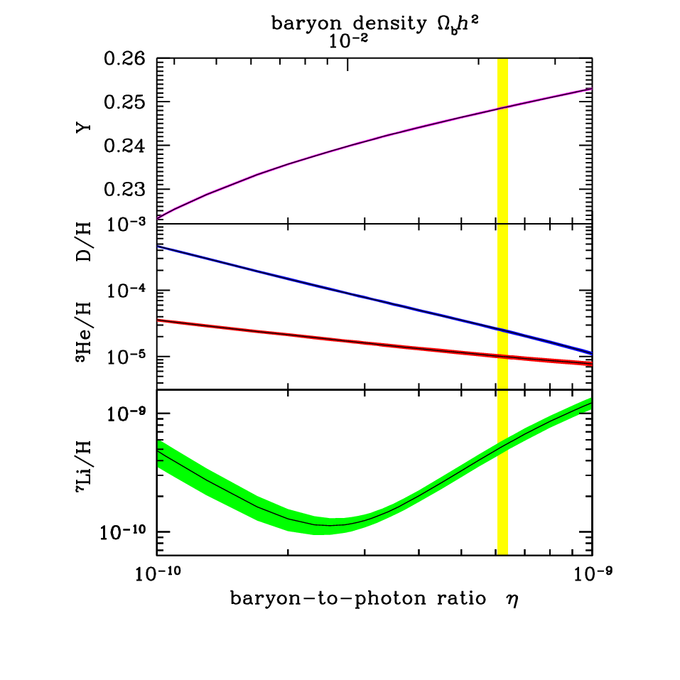
In standard BBN with , the only free parameter is the density of baryons (strictly speaking, nucleons), which sets the rates of the strong reactions. Because standard BBN is a one-parameter theory, any abundance measurement determines , while additional measurements overconstrain the theory and thereby provide a consistency check. BBN has thus historically been the premier means of determining the cosmic baryon density.
The release of the first-year WMAP results on the anisotropy spectrum of the CMB were a landmark event for all of cosmology, but particularly for BBN. As discussed above, the value of has been fixed by CMB measurements as given by Eq. (90). Thus, within the context of the Standard Model, BBN becomes a zero-parameter theory, and the light element predictions are completely determined to within the uncertainties in and the BBN theoretical errors. Comparison with light element observations then can be used to restate the test of BBN–CMB consistency, or to turn the problem around and test the astrophysics of post-BBN light element evolution [78].
0.3.2 Light element observations and comparison with theory
BBN theory predicts the abundances of D, , , and , which are essentially determined at s. Abundances are, however, observed at much later epochs, after stellar nucleosynthesis has commenced. The ejecta from stellar processing can alter the light element abundances from their primordial values, but also produce heavy elements such as C, N, O, and Fe (‘metals’). Thus one seeks astrophysical sites with low metal abundances, in order to measure light element abundances which are closer to primordial. For all of the light elements, systematic errors are an important and often dominant limitation to the precision of the primordial abundances.
D/H
In recent years, high-resolution spectra have revealed the presence of D in high-redshift, low-metallicity quasar absorption systems (QAS), via its isotope-shifted Lyman- absorption. These are the first measurements of light element abundances at cosmological distances. It is believed that there are no astrophysical sources of deuterium [65], so any measurement of D/H provides a lower limit to primordial D/H and thus an upper limit on . Recent observations by FUSE show a wide dispersion in the deuterium abundance in local gas seen via its absorption, [79]. This surprisingly large spread, taken together with the positive correlation of D/H with temperature and metallicity along various sightlines, led [79] to suggestions that deuterium may suffer significant and preferential depletion onto dust grains. In this case the true local interstellar D/H value would lie at the upper limit of the observed values, giving . However, extracting a primordial deuterium value requires a Galactic chemical evolution model (e.g., Ref. [80]), whose model dependences yield uncertainties in the determination of the primordial deuterium abundance. Many of these models do not predict significant D/H depletion [81] at high redshift, and in this case the high-redshift measurements are expected to recover the primordial deuterium abundance.
The deuterium abundance at low metallicity has been measured in several quasar absorption systems [82]. The weighted mean value of the seven systems with reliable abundance determinations is D/H where the error includes a scale factor of 1.72 and corresponds to D/H = . These are shown in Fig. 12. Since the D/H shows considerable scatter it is likely that systematic errors dominate the uncertainties. In this case it may be more appropriate to derive the uncertainty using sample variance (see, for example, Ref. [66]) which gives a more conservative range D/H or D/H = .

Using the WMAP value for the baryon density (90), the primordial D/H abundance is predicted to be [77]
| (110) |
As one can see from Fig. 11, this is in good agreement with the average of the seven best determined quasar absorption system abundances noted above, particularly when systematic uncertainties are taken into account.
We observe in clouds of ionized hydrogen (H II regions), the most metal-poor of which are in dwarf galaxies. There is now a large body of data on and CNO in these systems [83]. These data confirm that the small stellar contribution to helium is positively correlated with metal production. Recently a careful study of the systematic uncertainties in , particularly the role of underlying absorption, has led to a higher value for the primordial abundance of [84]. Using a subset of the highest quality from the data of Izotov and Thuan [83], all of the physical parameters listed above including the abundance were determined self-consistently with Monte Carlo methods [85]. The extrapolated abundance was determined to be . Conservatively, it would be difficult at this time to exclude any value of inside the range 0.232–0.258.
At the WMAP value for , the abundance is predicted to be [77]
| (111) |
This is in excellent agreement with the most recent analysis of the abundance [84]. Note also that the large uncertainty ascribed to this value indicates that while is certainly consistent with the WMAP determination of the baryon density, it does not provide for a highly discriminatory test of the theory at this time.
The systems best suited for Li observations are metal-poor stars in our Galaxy. Observations have long shown [86] that Li does not vary significantly in Pop II stars with metallicities of solar — the ‘Spite plateau’. Precision data suggest a small but significant correlation between Li and Fe [87] which can be understood as the result of Li production from Galactic cosmic rays [88]. Extrapolating to zero metallicity one arrives at a primordial value [89] .

Figure 13 shows the different Li components for a model with (/H) as a function of the iron abundance expressed as the log of Fe/H relative to the solar value. The linear slope produced by the model is independent of the input primordial value. The model [90] includes, in addition to primordial , lithium produced in Galactic cosmic-ray nucleosynthesis (primarily fusion), and produced by the -process during type II supernovae. As one can see, these processes are not sufficient to reproduce the population I abundance of (at near solar [Fe/H] ), and additional production sources are needed.
A recent reanalysis of the reaction, which is the most important production process in BBN, was considered in detail in Ref. [91]. When the new rate is used a high abundance is found [77] at the WMAP value of
| (112) |
This represents a 23% increase in over previous calculations [73]. The increase is primarily due to an increase in the () cross section. Newer data [91] implies 17% increase in this reaction leading to a 16% increase in . In addition, the 1.5% increase in from the 3-year to 5-year WMAP data [2] leads to a 3% increase in and finally another 1% increase is due to updated rates. In addition, the uncertainty in the BBN abundance is roughly a factor of 2 times smaller than previous determinations. This value for primordial is in clear contradiction with most estimates of the primordial Li abundance. Several attempts at explaining this discrepancy by adjusting some of the key nuclear rates have proved unsuccessful [71, 92, 93].
An important source for systematic error lies in the derived effective temperature of the star. [Li] is very sensitive to the temperature, with 0.065 – 0.08. Unfortunately there is no standard for determining effective temperatures, and, for a given star, there is considerable range depending on the method used. This spread in temperatures was made manifest in the recent work of Melendez and Ramirez [94] using the infra-red flux method (IRFM) which showed differences for very low metallicities ([Fe/H] -3) by as much as 500 K, with typical differences of K with respect to that of Ref. [87]. As a consequence the derived abundance was significantly higher with [94, 95].
Recently a dedicated set of observations were performed with the specific goal of determining the effective temperature in metal-poor stars [96]. Using a large set of Fe I excitation lines ( lines per star), the Boltzmann equation was used with the excitation energies, to determine the temperature through the distribution of excited levels. Again, there was no evidence for the high temperatures reported in Ref. [94], rather, temperatures were found to be consistent with previous determinations. The mean abundance found in Ref. [96] was , consistent with the bulk of prior abundance determinations.
There are of course other possible sources of systematic uncertainty in the abundance. It is possible that some of the surface has been depleted if the outer layers of the stars have been transported deep enough into the interior, and/or mixed with material from the hot interior; this may occur due to convection, rotational mixing, or diffusion. Estimates for possible depletion factors are in the range 0.2–0.4 dex, i.e., factors of 1.6–2.5 [97]. Recent attempts to deplete the abundance through diffusion introduce a source of turbulence tuned to fit the abundances of heavy elements in NGC6397 [98]. Once parameters are set, the degree of lithium depletion becomes a prediction of the model. For this cluster, a depletion factor of 0.25 dex is found, i.e., a factor of 1.8. Note that while this depletion factor would bring the previous BBN result of /H = [73] to a value close the value observed in that cluster [99] (), a larger depletion factor is needed with the new BBN value for given above. It is also not clear whether this mechanism will work for the wide range of stellar parameters seen in the field. As noted above, the Li data show a negligible intrinsic spread in Li. Any mechanism which reduces significantly the abundance of must do so uniformly over a wide range of stellar parameters (temperature, surface gravity, metallicity, rotational velocity, etc.).
It is also possible that the lithium discrepancy is a sign of new physics beyond the Standard Model. One possibility is the cosmological variation of the fine structure constant. Varying would induce a variation in the deuterium binding energy and could yield a decrease in the predicted abundance of [100]. A potential solution to both lithium problems is particle decay after BBN which could lower the abundance (and produce some as well) [101]. This has been investigated in the framework of the constrained minimal supersymmetric Standard Model if the lightest supersymmetric particle is assumed to be the gravitino [102] and indeed, some models have been found which accomplish these goals [103].
Since is also quite sensitive to the baryon density, one might hope that it too could be used as a baryometer. Observations of H II regions in our own Galaxy yield values of the /H ratio that are compatible with calculations of the primordial value [104, 105]. However, the extrapolation from the observations to a primordial abundance is complicated by the unknown chemical evolution of . Indeed, one does not even know whether /H is increasing or decreasing with cosmic time. Thus a primordial extrapolation yields only an order-of-magnitude range of allowable values of /H [106].
0.3.3 Beyond the Standard Model
Given the simple physics underlying BBN, it is remarkable that it still provides one of the most effective tests for physics beyond the Standard Model. Limits on particle physics beyond the Standard Model come mainly from the observational bounds on the abundance. As discussed earlier, the neutron-to-proton ratio is fixed by its equilibrium value at the freeze-out of the weak interaction rates at a temperature MeV modulo the occasional free neutron decay. Furthermore, freeze-out is determined by the competition between the weak interaction rates and the expansion rate of the Universe
| (113) |
In the Standard Model, the number of relativistic particle species at 1 MeV is . The presence of additional neutrino flavours (or any other relativistic species) at the time of nucleosynthesis increases the overall energy density of the Universe and hence the expansion rate leading to a larger value of , , and ultimately . Because of the form of Eq. (113) it is clear that just as one can place limits [107] on , any changes in the weak or gravitational coupling constants can be similarly constrained (for a discussion see Ref. [108]).
The helium curve in Fig. 11 was computed taking ; the computed abundance scales as [61]. The dependence of the light element abundances on is shown in Fig. 14 [78]. For a fixed value of (slightly below the current WMAP value) and , the likelihood distribution for is shown by the shaded region in Fig. 15 [109]. Also shown for comparison are the likelihood distribution based the WMAP value of using D/H alone, and D/H, and the result based on BBN alone. Despite the increased uncertainty in the He abundance, it still provides the strongest constraint on . D/H is nonetheless becoming competitive in its ability to set limits on .


The 95 % CL upper limits to are given in Table 4. In all cases the preferred values for are consistent with , and in many cases are much closer to than . This restates the overall consistency among standard BBN theory, D and observations, and CMB anisotropies. It also constrains departures from this scenario. The combined limit using BBN + light elements + CMB limit is [109]
| (114) |
at 68% CL.
| Observations | |||
|---|---|---|---|
| + D/HA | 1.59 | ||
| + | 1.63 | ||
| D/HA + | 2.78 | ||
| + D/HA + | 1.44 |
0.4 Lecture 4: Dark Matter
Evidence for dark matter in the Universe is available from a wide range of observational data. As discussed many times above, the analysis of the cosmic microwave background anisotropies leads to the conclusion that the curvature of the Universe is close to zero indicating that the sum of the fractions of critical density, , in matter and a cosmological constant (or dark energy) is very close to one [2]. When combined with a variety of data including results from the analysis of type Ia supernovae observations [26, 27] and baryon acoustic oscillations [28] one is led to the concordance model where and with the remainder (leading to ) in baryonic matter. This is in addition to the classic evidence from galactic rotation curves [110], which indicate that nearly all spiral galaxies are embedded in a large galactic halo of dark matter leading to rather constant rotational velocities at large distances from the centre of the galaxy (in contrast to the expected behaviour in the absence of dark matter). Other dramatic pieces of evidence can be found in combinations of X-ray observations and weak lensing showing the superposition of dark matter (from lensing) and ordinary matter from X-ray gas [111] and from the separation of baryonic and dark matter after the collision of two galaxies as seen in the Bullet cluster [112]. For a more complete discussion see Ref. [113].
From the first column of Table 2, we can obtain the density of cold dark matter from the difference between the total matter density and the baryon density [2]
| (115) |
or a 2 range of 0.0975–0.1223 for .
0.4.1 Neutrinos
Dark matter must be both long-lived or stable and electrically and colour neutral. As a result, once baryons and neutrinos are eliminated as candidates, one must look beyond the Standard Model. From WMAP, we already know that the baryon density is far below the requisite amount in cold dark matter. Light neutrinos () are a long-time standard when it comes to non-baryonic dark matter [114]. Light neutrinos are, however, ruled out as a dominant form of dark matter because they produce too much large scale structure [115]. The energy of density of light neutrinos with MeV can be expressed at late times as . Imposing the constraint , translates into a strong constraint (upper bound) on Majorana neutrino masses [116]:
| (116) |
where the sum runs over neutrino mass eigenstates. The limit for Dirac neutrinos depends on the interactions of the right-handed states. The limit (116) and the corresponding initial rise in as a function of is displayed in Fig. 16. Much stronger limits on the sum of neutrino masses are possible when combining the WMAP data with large scale structure surveys. A typical limit is eV or [2].

The calculation of the relic density for neutrinos more massive than MeV, is substantially more involved. The relic density is now determined by the freeze-out of neutrino annihilations which occur at , after annihilations have begun to seriously reduce their number density [118]. For particles which annihilate through approximate weak scale interactions, annihilations freeze out when .
Based on the leptonic and invisible width of the boson, experiments at LEP have determined that the number of neutrinos is [119]. Thus, LEP excludes additional neutrinos (with standard weak interactions) with masses GeV. The mass density of ordinary heavy neutrinos is found to be very small, for masses GeV up to TeV [118]. Laboratory constraints for Dirac neutrinos are available [120], excluding neutrinos with masses between 10 GeV and 4.7 TeV. This is significant, since it precludes the possibility of neutrino dark matter based on an asymmetry between and [121].
0.4.2 Axions
Owing to space limitations, the discussion of axions as a dark matter candidate will be very brief. Axions are pseudo-Goldstone bosons which arise in solving the strong CP problem [122, 123] via a global U(1) Peccei–Quinn symmetry. The invisible axion [123] is associated with the flat direction of the spontaneously broken PQ symmetry. Because the PQ symmetry is also explicitly broken (the CP violating coupling is not PQ invariant), the axion picks up a small mass similar to a pion picking up a mass when chiral symmetry is broken. We can expect that where , the axion decay constant, is the vacuum expectation value of the PQ current and can be taken to be quite large. If we write the axion field as , near the minimum, the potential produced by QCD instanton effects looks like . The axion equations of motion lead to a relatively stable oscillating solution. The energy density stored in the oscillations exceeds the critical density [124] unless GeV.
Axions may also be emitted from stars and supernovae [125]. In supernovae, axions are produced via nucleon–nucleon bremsstrahlung with a coupling . As was noted above, the cosmological density limit requires GeV. Axion emission from red giants imply [126] GeV (though this limit depends on an adjustable axion–electron coupling), the supernova limit requires [127] GeV for naive quark model couplings of the axion to nucleons. Thus only a narrow window exists for the axion as a viable dark matter candidate.
0.4.3 Neutralinos
Supersymmetry is one of the best-motivated proposals for physics beyond the Standard Model. It is well known that supersymmetry could help stabilize the mass scale of electroweak symmetry breaking by cancelling the quadratic divergences in the radiative corrections to the mass-squared of the Higgs boson [128]. In addition, including supersymmetric partners of Standard Model particles in the renormalization-group equations (RGEs) for the gauge couplings of the Standard Model would permit them to unify [129], whereas unification would not occur if only the Standard Model particles were included in the RGEs.
To construct the supersymmetric Standard Model [130] we start with the complete set of chiral fermions needed in the Standard Model, and add a scalar superpartner to each Weyl fermion so that each field in the Standard Model corresponds to a chiral multiplet. Similarly we must add a gaugino for each of the gauge bosons in the Standard Model making up the gauge multiplets. The Minimal Supersymmetric Standard Model (MSSM) [131] is defined by its minimal field content (which accounts for the known Standard Model fields) and minimal superpotential necessary to account for the known Yukawa mass terms. As such we define the MSSM by the superpotential
| (117) |
In Eq. (117), the indices are SU(2)L doublet indices. The Yukawa couplings are all matrices in generation space. Note that there is no generation index for the Higgs multiplets. Colour and generation indices have been suppressed in the above expression. There are two Higgs doublets in the MSSM. This is a necessary addition to the Standard Model which can be seen as arising from the holomorphic property of the superpotential. That is, there would be no way to account for all of the Yukawa terms for both up-type and down-type multiplets with a single Higgs doublet. To avoid a massless Higgs state, a mixing term must be added to the superpotential.
In defining the MSSM, we have limited the model to contain a minimal field content: the only new fields are those which are required by supersymmetry. Consequently, apart from superpartners, only the Higgs sector was enlarged from one doublet to two. Moreover, in writing the superpotential (117), we have also made a minimal choice regarding interactions. We have limited the types of interactions to include only the minimal set required in the Standard Model and its supersymmetric generalization. There are, however, additional superpotential terms which are consistent with gauge invariance. These would lead to rapid baryon and/or lepton number violation and can be eliminated by imposing a discrete symmetry on the theory called -parity [132]. This can be represented as
| (118) |
where , and are the baryon number, lepton number, and spin, respectively. It is easy to see that, with the definition (118), all the known Standard Model particles have -parity +1. For example, the electron has , , and , and the photon has and , so in both cases . Similarly, it is clear that all superpartners of the known Standard Model particles have , since they must have the same value of and as their conventional partners, but differ by 1/2 unit of spin. If -parity is exactly conserved, then the additional superpotential terms must be absent from the theory. An immediate result of imposing -parity is the stability of the lightest sparticle making it a potential dark matter candidate. Possible choices for the lightest supersymmetric particle (LSP) are the neutralino, sneutrino, and gravitino. Here, I will focus only on the former.
There are four neutralinos, each of which is a linear combination of the neutral fermions [133]: the wino , the partner of the third component of the gauge boson; the bino, ; and the two neutral Higgsinos, and . The mass and composition of the LSP are determined by the gaugino masses, , and . In general, neutralinos can be expressed as a linear combination
| (119) |
The solution for the coefficients and for neutralinos that make up the LSP can be found by diagonalizing the mass matrix
| (120) |
where is a soft supersymmetry breaking term giving mass to the U(1) (SU(2)) gaugino(s).
The relic density of neutralinos depends on additional parameters in the MSSM beyond , and . These include the sfermion masses and the Higgs pseudo-scalar mass . To determine the relic density it is necessary to obtain the general annihilation cross-section for neutralinos. In much of the parameter space of interest, the LSP is a bino and the annihilation proceeds mainly through sfermion exchange.
In its generality, the minimal supersymmetric standard model (MSSM) has over 100 undetermined parameters. There are good arguments based on grand unification [129] and supergravity [134] which lead to a strong reduction in the number of parameters. I will assume several unification conditions placed on the supersymmetric parameters. In all models considered, the gaugino masses are assumed to be unified at the GUT scale with value as are the trilinear couplings with value . Also common to all models considered here is the unification of all soft scalar masses set equal to at the GUT scale. With this set of boundary conditions at the GUT scale, we can use the radiative electroweak symmetry breaking conditions by specifying the ratio of the two Higgs vacuum expectation values, , and the mass to predict the values of the Higgs mixing mass parameter and Higgs pseudoscalar mass . The sign of remains free. This class of models is often referred to as the constrained MSSM (CMSSM) [135, 136, 137, 138, 139]. In the CMSSM, the solutions for generally lead to a lightest neutralino which is very nearly a pure .
In Fig. 17, an example of the renormalization group running of the mass parameters in the CMSSM is shown. Here, we have chosen GeV, GeV, , , and . Indeed, it is rather amazing that, from so few input parameters, all of the masses of the supersymmetric particles can be determined. The characteristic features that one sees in the figure are, for example, that the coloured sparticles are typically the heaviest in the spectrum. This is due to the large positive correction to the masses due to in the RGEs. Also, one finds that the is typically the lightest sparticle. But most importantly, notice that one of the Higgs mass2 goes negative triggering electroweak symmetry breaking [140]. (The negative sign in the figure refers to the sign of the mass squared, even though it is the mass of the sparticles which is depicted.)

For a given value of , , and , the resulting regions of parameter space with acceptable relic density and which satisfy the phenomenological constraints can be displayed on the plane. In Fig. 18(a), the light shaded region corresponds to that portion of the CMSSM plane with , , and such that the computed relic density yields the WMAP value given in Eq. (115) [138]. The bulk region at relatively low values of and , tapers off as is increased. At higher values of , annihilation cross sections are too small to maintain an acceptable relic density and is too large. Although sfermion masses are also enhanced at large (due to RGE running), co-annihilation processes between the LSP and the next lightest sparticle (in this case the ) enhance the annihilation cross section and reduce the relic density. This occurs when the LSP and NLSP are nearly degenerate in mass. The dark shaded region has and is excluded. The effect of co-annihilations is to create an allowed band about 25–50 GeV wide in for GeV, or GeV, which tracks above the contour [141].


Also shown in Fig. 18(a) are the relevant phenomenological constraints. These include the LEP limits on the chargino mass: GeV [142]; on the selectron mass: GeV [143]; and on the Higgs mass: GeV [144]. The former two constrain and directly via the sparticle masses, and the latter indirectly via the sensitivity of radiative corrections to the Higgs mass to the sparticle masses, principally . FeynHiggs [145] is used for the calculation of . The Higgs limit imposes important constraints principally on particularly at low . Another constraint is the requirement that the branching ratio for be consistent with the experimental measurements [146]. These measurements agree with the Standard Model, and therefore provide bounds on MSSM particles [147] such as the chargino and charged Higgs masses, in particular. Typically, the constraint is more important for , but it is also relevant for , particularly when is large. The constraint imposed by measurements of also excludes small values of . Finally, there are regions of the plane that are favoured by the BNL measurement [148] of at the 2- level, corresponding to a deviation from the Standard Model calculation [149].
Another mechanism for extending the allowed regions in the CMSSM to large is rapid annihilation via a direct-channel pole when [135, 137]. Since the heavy scalar and pseudoscalar Higgs masses decrease as increases, eventually yielding a ‘funnel’ extending to large and at large , as seen in Fig. 18(b). As one can see, the impact of the Higgs mass constraint is reduced (relative to the case with ) while that of is enhanced.
Shown in Fig. 19 are the WMAP lines [138] of the plane for and values of from 5 to 55, in steps . We notice immediately that the strips are considerably narrower than the spacing between them, though any intermediate point in the plane would be compatible with some intermediate value of . The right (left) ends of the strips correspond to the maximal (minimal) allowed values of and hence . The lower bounds on are due to the Higgs mass constraint for , but are determined by the constraint for higher values of .

Finally, there is one additional region of acceptable relic density known as the focus-point region [150], which is found at very high values of . An example showing this region is found in Fig. 20, plotted for , , and GeV. As is increased, the solution for at low energies as determined by the electroweak symmetry breaking conditions eventually begins to drop. When , the composition of the LSP gains a strong Higgsino component and as such the relic density begins to drop precipitously. As is increased further, there are no longer any solutions for . This occurs in the shaded region in the upper left corner of Fig. 20. The position of the focus point strip is very sensitive to the value of [151].

As seen in Fig. 18, the relic density constraint is compatible with relatively large values of and . However, all values of and are not equally viable when the available phenomenological and cosmological constraints are taken into account. A global likelihood analysis enables one to pin down the available parameter space in the CMSSM. One can avoid the dependence on priors by performing a pure likelihood analysis as in Ref. [152], or a purely -based fit as done in Refs. [153, 154]. Here we present results from one such analysis [155, 156], which used a Markov–Chain Monte Carlo (MCMC) technique to explore efficiently the likelihood function in the parameter space of the CMSSM. A full list of the observables and the values assumed for them in this global analysis are given in Ref. [154], and updated in Refs. [155, 156].
The 68% and 95% confidence-level (CL) regions in the plane of the CMSSM is shown in Fig. 21 [155]. Also shown for comparison are the physics reaches of ATLAS and CMS with 1/fb of integrated luminosity [157, 158]. (MET stands for missing transverse energy, SS stands for same-sign dilepton pairs, and the sensitivity for finding the lightest Higgs boson in cascade decays of supersymmetric particles is calculated for 2/fb of data.) The likelihood analysis assumed , as motivated by the sign of the apparent discrepancy in , but sampled all values of and : the experimental sensitivities were estimated assuming and , but are probably not very sensitive to these assumptions. The global maximum of the likelihood function (indicated by the black dot) is at GeV, GeV, GeV, , and (37% probability). It is encouraging that the best-fit point lies well within the LHC discovery range, as do the 68% and most of the 95% CL regions.
Improvements in sensitivity have made it possible for direct detection experiments [159, 160] to be competitive with other phenomenological constraints. The elastic cross section for scattering on a nucleus can be decomposed into a scalar (spin-independent) and a spin-dependent part. Each of these can be written in terms of the cross sections for elastic scattering off individual nucleons. The scalar part of the cross section can be written as
| (121) |
where is the -nuclear reduced mass and
| (122) |
for = p or n. The parameters are defined by
| (123) |
and the contain the individual quark-neutralino scattering cross sections, see Refs. [161, 162, 163] for further details regarding the calculation of the cross section.
The elastic scattering of neutralinos on nucleons is very sensitive to the strangeness contribution to the nucleon mass and can be characterized by the parameter which is also related to the -nucleon sigma term by
| (124) |
where is the change in the nucleon mass due to non-zero and masses and is estimated from octet baryon mass differences to be MeV [164], and the latest determination of MeV. The effects of varying these assumptions are discussed in the context of the CMSSM in Refs. [162, 163]. Lattice calculations are now reaching the stage where they may also provide useful information on [165], and a recent analysis would suggest a lower value [166].
In Fig. 22(a) we show CMSSM spin-independent neutralino-nucleon cross section, as obtained in a scan over all CMSSM parameters with , 100 GeV, 0 GeV GeV, and [167]. We also allow both positive and negative , except for large , where convergence becomes difficult in the case. At low GeV, cross sections generally exceed pb, and the largest scalar cross sections, which occur for GeV, are already excluded by CDMS II [159] and/or XENON10 [160]. These exclusions occur primarily in the focus-point region at large . On the other hand, for GeV, scalar cross sections are well below pb, and come from the co-annihilation strip or the rapid-annihilation funnel that appears at large in the CMSSM. The effective cross sections shown are suppressed for points with , and there may be cancellations at larger that suppress the cross sections substantially. These regions of parameter space will not be probed by direct detection experiments in the near future [168, 169]. The corresponding 68% and 95% CL regions in the cross section–neutralino mass plane from the frequentist analysis of Ref. [156] are shown in Fig. 22(b).


Acknowledgements
This work was supported in part by DOE grant DE-FG02-94ER-40823
References
- [1] S. Weinberg, Gravitation and Cosmology (Wiley, New York, 1972).
- [2] J. Dunkley et al. [WMAP Collaboration], Astrophys. J. Suppl. 180 (2009) 306 [arXiv:0803.0586 [astro-ph]]; E. Komatsu et al. [WMAP Collaboration], Astrophys. J. Suppl. 180 (2009) 330 [arXiv:0803.0547 [astro-ph]].
- [3] J.C. Mather et al., Astrophys. J. 512 (1999) 511.
- [4] P.J.E. Peebles, Principles of Physical Cosmology (Princeton University Press, 1993).
- [5] G. Börner, The Early Universe: Facts and Fiction (Springer-Verlag, Berlin, 1988).
- [6] J.A. Peacock, Cosmological Physics (Cambridge University Press, 1999).
- [7] V. Mukhanov, Physical Foundations of Cosmology (Cambridge University Press, 2005).
- [8] S. Weinberg, Cosmology (Oxford University Press, 2008).
- [9] K.A. Olive and J.A. Peacock, in C. Amsler et al. [Particle Data Group], Phys. Lett. B667 (2008) 217–227.
- [10] G. Gamow, Phys. Rev. 74 (1948) 505; G. Gamow, Nature 162 (1948) 680; R.A. Alpher and R.C. Herman, Nature 162 (1948) 774.
- [11] R. A. Alpher and R. C. Herman, Phys. Rev. 74, 1737 (1948); Phys. Rev. 75 (1949)1089.
- [12] A. A. Penzias and R. W. Wilson, Astrophys. J. 142 (1965) 419.
- [13] R. H. Dicke, P. J. E. Peebles, P. G. Roll and D. T. Wilkinson, Astrophys. J. 142 (1965) 414.
- [14] G.F. Smoot et al., Astrophys. J. 396 (1992) L1; E.L. Wright et al., Astrophys. J. 396 (1992) L13.
- [15] A. T. Lee et al., Astrophys. J. 561 (2001) L1 [arXiv:astro-ph/0104459]; R. Stompor et al., Astrophys. J. 561 (2001) L7 [arXiv:astro-ph/0105062].
- [16] W. C. Jones et al., Astrophys. J. 647 (2006) 823 [arXiv:astro-ph/0507494].
- [17] N. W. Halverson et al. Mon. Not. Roy. Astron. Soc. 568 (2002) 38 [arXiv:astro-ph/0104489]; C. Pryke, N. W. Halverson, E. M. Leitch, J. Kovac, J. E. Carlstrom, W. L. Holzapfel and M. Dragovan, Astrophys. J. 568 (2002) 46 [arXiv:astro-ph/0104490].
- [18] S. Padin, et al., Astrophys. J. 549 (2001) L1; T.J. Pearson et al., Astrophys. J. 591 (2003) 556; J. L. Sievers et al., arXiv:0901.4540 [astro-ph.CO].
- [19] J. A. Rubino-Martin et al., Mon. Not. Roy. Astron. Soc. 341 (2003) 1084 [arXiv:astro-ph/0205367].
- [20] A. Benoit et al. [the Archeops Collaboration], Astron. Astrophys. 399 (2003) L25 [arXiv:astro-ph/0210306]; M. Tristram et al., Astron. Astrophys. 436 (2005) 785 [arXiv:astro-ph/0411633].
- [21] C. L. Bennett et al., Astrophys. J. Suppl. 148 (2003) 1; D. N. Spergel et al., Astrophys. J. Suppl. 148 (2003) 175.
- [22] C. l. Kuo et al. [ACBAR Collaboration], Astrophys. J. 600 (2004) 32 [arXiv:astro-ph/0212289]; C. L. Reichardt et al., Astrophys. J. 694 (2009) 1200 [arXiv:0801.1491 [astro-ph]].
- [23] R. B. Friedman et al. [QUaD Collaboration], Astrophys. J. 700, L187 (2009) [arXiv:0901.4334 [astro-ph.CO]].
- [24] D. Scott and G. F. Smoot, in C. Amsler et al. [Particle Data Group], Phys. Lett. B667 (2008) 1.
- [25] O. Lahav and A. R. Liddle, in C. Amsler et al. [Particle Data Group], Phys. Lett. B667 (2008) 1.
- [26] A.G. Riess et al., Astronom. J. 116 (1998) 1009; P. Garnavich et al., Astrophys. J. 509 (1998) 74; S. Perlmutter et al., Astrophys. J. 517 (1999) 565; A. G. Riess et al., Astrophys. J. 560 (2001) 49; J.L. Tonry et al., Astrophys. J. 594 (2003) 1; A.G. Riess et al., Astrophys. J. 659 (2007) 98.
- [27] P. Astier et al. [The SNLS Collaboration], Astron. Astrophys. 447 (2006) 31 [arXiv:astro-ph/0510447].
- [28] D. Eisenstein et al., Astrophys. J. 633, 560 (2005); C. Blake et al., Mon. Not. Roy. Astron. Soc. 374, 1527 (2007); W. J. Percival, et al., Mon. Not. Roy. Astron. Soc. 381 (2007) 1053.
- [29] M. Kowalski et al., Astrophys. J. 686, 749 (2008).
- [30] W. Rindler, Mon. Not. Roy. Astron. Soc. 116 (1956) 663; G.F.R. Ellis and W. Stoeger, Class. Quantum Grav. 5 (1988) 207.
- [31] S.K. Blau and A.H. Guth, in 300 Years of Gravitation, Eds. S.W. Hawking and W. Israel (Cambridge University Press, 1987).
- [32] G. t’Hooft, Nucl. Phys. B79 (1974) 276; A.M. Polyakov, JETP Lett. 20 (1974) 194.
- [33] T.W.B. Kibble, J. Phys. A9 (1976) 1387.
- [34] Ya. B. Zeldovich and M.Y. Khlopov, Phys. Lett. 79B (1979) 239; J.P. Preskill, Phys. Rev. Lett. 43 (1979) 1365.
- [35] A.H. Guth, Phys. Rev. D23 (1981) 347.
- [36] for reviews see: A. D. Linde, Particle Physics and Inflationary Cosmology (Harwood, Chur, Switzerland, 1990); K. A. Olive, Phys. Rep. 190 (1990) 307; D. H. Lyth and A. Riotto, Phys. Rep. 314 (1999) 1 [arXiv:hep-ph/9807278].
- [37] W.H. Press, Phys. Scr. 21 (1980) 702; V.F. Mukhanov and G.V. Chibisov, JETP Lett. 33 (1981) 532; S.W. Hawking, Phys. Lett. 115B (1982) 295; A.A. Starobinsky, Phys. Lett. 117B (1982) 175; A.H. Guth and S.Y. Pi, Phys. Rev. Lett. 49 (1982) 1110; J.M. Bardeen, P.J. Steinhardt and M.S. Turner, Phys. Rev. D28 (1983) 679.
- [38] S. Coleman, Phys. Rev. D15 (1977) 2929; C.G. Callan and S. Coleman, Phys. Rev. D16 (1977) 1762.
- [39] A.H. Guth and E.J. Weinberg, Phys. Rev. D23 (1981) 876; Nucl. Phys. 212 (1983) 321.
- [40] A.D. Linde, Phys. Lett. 108B (1982) 389; A. Albrecht and P.J. Steinhardt, Phys. Rev. Lett. 48 (1982) 1220.
- [41] S. Coleman and E. Weinberg, Phys. Rev. D7 (1973) 1888; A.D. Linde, JETP Lett. 23 (1976) 64.
- [42] A.D. Linde, Phys. Lett. 114B (1982) 431.
- [43] A.D. Linde, Phys. Lett. 116B (1982) 335.
- [44] B. Campbell, S. Davidson, and K.A. Olive, Nucl. Phys. B399 (1993) 111.
- [45] J. Ellis, K. Enqvist, D.V. Nanopoulos, and K.A. Olive, Phys. Lett. B191 (1987) 343.
- [46] A.D. Linde, Phys. Lett. 129B (1983) 177.
- [47] A.D. Linde, in 300 Years of Gravitation, Eds. S.W. Hawking and W. Israel (Cambridge University Press, 1987).
- [48] G. Steigman, Annu. Rev. Astron. Astrophys. 14 (1976) 339.
- [49] A.D. Sakharov, JETP Lett. 5 (1967) 24.
- [50] S. Weinberg, Phys. Rev. Lett. 42 (1979) 850; D. Toussaint, S. B. Treiman, F. Wilczek, and A. Zee, Phys. Rev. D19 (1979) 1036.
- [51] J.N. Fry, K.A. Olive, and M.S. Turner, Phys. Rev. D22 (1980) 2953; D22 (1980) 2977; Phys. Rev. Lett. 45 (1980) 2074.
- [52] E.W. Kolb and S. Wolfram, Phys. Lett. B91 (1980) 217; Nucl. Phys. B172 (1980) 224.
- [53] for reviews see: E.W. Kolb and M.S. Turner, Annu. Rev. Nucl. Part. Sci. 33 (1983) 645; A. Dolgov, Phys. Rep. 222 (1993) 309.
- [54] S. M. Barr, G. Segre and H. A. Weldon, Phys. Rev. D20 (1979) 2494; A. Yildiz and P. H. Cox, Phys. Rev. D21 (1980) 906.
- [55] I. Affleck and M. Dine, Nucl. Phys. B249 (1985) 361.
- [56] P. Minkowski, Phys. Lett. B67 (1977) 421; M. Gell-Mann, P. Ramond, and R. Slansky, in Supergravity, Eds. D.Z. Freedman and P. van Nieuwenhuizen (North Holland, Amsterdam, 1979); T. Yanagida, in Proceedings of the Workshop on the Unified Theory and the Baryon Number of the Universe, Eds. O. Sawada and S. Sugamoto, KEK79-18 (1979).
- [57] M. Fukugita and T. Yanagida, Phys. Lett. B174 (1986) 45.
- [58] V. Kuzmin, V. Rubakov and M. Shaposhnikov, Phys. Lett. B155 (1985) 36.
- [59] T. P. Walker, G. Steigman, D. N. Schramm, K. A. Olive and K. Kang, Astrophys. J. 376 (1991) 51; K. A. Olive, G. Steigman, and T. P. Walker, Phys. Rep. 333 (2000) 389; B. D. Fields and K. A. Olive, Nucl. Phys. A777 (2006) 208; B. D. Fields and S. Sarkar, in C. Amsler et al. [Particle Data Group], Phys. Lett. B667 (2008) 1.
- [60] R. H. Cyburt, B. D. Fields and K. A. Olive, Phys. Lett. B567 (2003) 227 [arXiv:astro-ph/0302431].
- [61] J. Bernstein, L. S. Brown and G. Feinberg, Rev. Mod. Phys. 61 (1989) 25.
- [62] V. Mukhanov, arXiv:astro-ph/0303073.
- [63] E.M. Burbidge, G.R. Burbidge, W.A. Fowler, and F. Hoyle, Rev. Mod. Phys. 29 (1957) 547.
- [64] B.D. Fields and K.A. Olive, Astrophys. J. 506 (1998) 177.
- [65] H. Reeves, J. Audouze, W.A. Fowler, and D.N. Schramm, Astrophys. J. 179 (1973) 909; R. I. Epstein, J. M. Lattimer, and D. N. Schramm, Nature 263 (1976) 198; T. Prodanović and B. D. Fields, Astrophys. J. 597 (2003) 48 [arXiv:astro-ph/0307183].
- [66] R. H. Cyburt, B. D. Fields and K. A. Olive, New Astron. 6 (2001) 215 [arXiv:astro-ph/0102179].
- [67] L.M. Krauss and P. Romanelli, Astrophys. J. 358 (1990) 47; M. Smith, L. Kawano, and R.A. Malaney, Astrophys. J. Suppl. 85 (1993) 219; N. Hata, R.J. Scherrer, G. Steigman, D. Thomas, and T.P. Walker, Astrophys. J. 458 (1996) 637.
- [68] K. M. Nollett and S. Burles, Phys. Rev. D61 (2000) 123505 [arXiv:astro-ph/0001440].
- [69] A. Coc, E. Vangioni-Flam, M. Cassé and M. Rabiet, Phys. Rev. D65 (2002) 043510 [arXiv:astro-ph/0111077].
- [70] C. Angulo et al. (NACRE Collaboration), Nucl. Phys. A 656 (1999) 3.
- [71] A. Coc, E. Vangioni-Flam, P. Descouvemont, A. Adahchour and C. Angulo, Astrophys. J. 600 (2004) 544 [arXiv:astro-ph/0309480].
- [72] G. Fiorentini, E. Lisi, S. Sarkar and F. L. Villante, Phys. Rev. D58 (1998) 063506 [arXiv:astro-ph/9803177]; S. Burles, K. M. Nollett and M. S. Turner, Astrophys. J. 552 (2001) L1 [arXiv:astro-ph/0010171].
- [73] R. H. Cyburt, Phys. Rev. D70 (2004) 023505 [arXiv:astro-ph/0401091].
- [74] M. Smith, L. Kawano, and R. A. Malaney, Astrophys. J. Suppl. 85 (1993) 219.
- [75] P. Descouvemont, A. Adahchour, C. Angulo, A. Coc and E. Vangioni-Flam, Atom. Data Nucl. Data Tables 88 (2004) 203 [arXiv:astro-ph/0407101].
- [76] A. Cuoco, F. Iocco, G. Mangano, G. Miele, O. Pisanti and P. D. Serpico, Int. J. Mod. Phys. A19 (2004) 4431 [arXiv:astro-ph/0307213]; P. D. Serpico, S. Esposito, F. Iocco, G. Mangano, G. Miele and O. Pisanti, JCAP 0412 (2004) 010 [arXiv:astro-ph/0408076].
- [77] R. H. Cyburt, B. D. Fields and K. A. Olive, JCAP 0811 (2008) 012 [arXiv:0808.2818 [astro-ph]].
- [78] R. H. Cyburt, B. D. Fields and K. A. Olive, Astropart. Phys. 17 (2002) 87 [arXiv:astro-ph/0105397].
- [79] J. L. Linsky et al., Astrophys. J. 647 (2006) 1106 [arXiv:astro-ph/0608308].
- [80] E. Vangioni-Flam, K. A. Olive and N. Prantzos, Astrophys. J. 427 (1994) 618 [arXiv:astro-ph/9310021]; S. Scully, M. Casse, K. A. Olive and E. Vangioni-Flam, Astrophys. J. 476 (1997) 521 [arXiv:astro-ph/9607106]; G. Steigman, D. Romano and M. Tosi, Mon. Not. Roy. Astron. Soc. 378 (2007) 576 [arXiv:astro-ph/0703682]; T. Prodanovic and B. D. Fields, JCAP 0809 (2008) 003 [arXiv:0804.3095 [astro-ph]].
- [81] D.D. Clayton, Astrophys. J. 290 (1985) 428; B.D. Fields, Astrophys. J. 456 (1996) 678.
- [82] M. Pettini, B. J. Zych, M. T. Murphy, A. Lewis and C. C. Steidel, Mon. Not. Roy. Astron, Soc. 391 (2008) 1499 [arXiv:0805.0594 [astro-ph]], and references therein.
- [83] Y.I. Izotov, T.X. Thuan, and V.A. Lipovetsky, Astrophys. J. 435 (1994) 647 ; Astrophys. J. Suppl. 108 (1997) 1 ; Y.I. Izotov, and T.X. Thuan, Astrophys. J. 500 (1998) 188 ; Y. I. Izotov and T. X. Thuan, Astrophys. J. 602 (2004) 200 [arXiv:astro-ph/0310421].
- [84] K. A. Olive and E. D. Skillman, Astrophys. J. 617 (2004) 29 [arXiv:astro-ph/0405588].
- [85] K. A. Olive and E. D. Skillman, New Astron. 6 (2001) 119.
- [86] F. Spite, and M. Spite, Astron. Astrophys. 115 (1982) 357; P. Molaro, F. Primas, and P. Bonifacio, Astron. Astrophys. 295 (1995) L47 ; P. Bonifacio and P. Molaro, Mon. Not. Roy. Astron, Soc. 285 (1997) 847.
- [87] S.G. Ryan, J.E. Norris, and T.C. Beers, Astrophys. J. 523 (1999) 654 .
- [88] B.D.Fields and K.A. Olive, New Astron. 4 (1999) 255; E. Vangioni-Flam, M. Cassé, R. Cayrel, J. Audouze, M. Spite, and F. Spite, New Astron. 4 (1999) 245 .
- [89] S.G. Ryan, T.C. Beers, K.A. Olive, B.D. Fields, and J.E. Norris, Astrophys. J. Lett. 530 (2000) L57 .
- [90] B.D. Fields and K.A. Olive, Astrophys. J. 516 (1999) 797.
- [91] R. H. Cyburt and B. Davids, Phys. Rev. C78 (2008) 064614 [arXiv:0809.3240 [nucl-ex]].
- [92] C. Angulo et al., Astrophys. J. 630 (2005) L105 [arXiv:astro-ph/0508454].
- [93] R. H. Cyburt, B. D. Fields and K. A. Olive, Phys. Rev. D69 (2004) 123519 [arXiv:astro-ph/0312629].
- [94] J. Melendez and I. Ramirez, Astrophys. J. 615 (2004) L33 [arXiv:astro-ph/0409383].
- [95] Consequences on the LiBeB elements of this temperature scale were considered in B. D. Fields, K. A. Olive and E. Vangioni-Flam, Astrophys. J. 623 (2005) 1083 [arXiv:astro-ph/0411728].
- [96] A. Hosford, S. G. Ryan, A. E. G. Perez, J. E. Norris and K. A. Olive, Astron. Astrophys. 493 (2009) 601 [arXiv:0811.2506 [astro-ph]].
- [97] S. Vauclair and C. Charbonnel, Astrophys. J. 502 (1998) 372 [arXiv:astro-ph/9802315]; M. H. Pinsonneault, T. P. Walker, G. Steigman and V. K. Narayanan, Astrophys. J. 527 (1998) 180 [arXiv:astro-ph/9803073]; M. H. Pinsonneault, G. Steigman, T. P. Walker, and V. K. Narayanan, Astrophys. J. 574 (2002) 398 [arXiv:astro-ph/0105439]; O. Richard, G. Michaud and J. Richer, Astrophys. J. 619 (2005) 538 [arXiv:astro-ph/0409672];
- [98] A. J. Korn et al., Nature 442 (2006) 657 [arXiv:astro-ph/0608201].
- [99] P. Bonifacio et al., Astron. Astrophys. 390 (2002) 91 [arXiv:astro-ph/0204332].
- [100] V. F. Dmitriev, V. V. Flambaum and J. K. Webb, Phys. Rev. D69 (2004) 063506 [arXiv:astro-ph/0310892]; A. Coc, N. J. Nunes, K. A. Olive, J. P. Uzan and E. Vangioni, Phys. Rev. D76 (2007) 023511 [arXiv:astro-ph/0610733].
- [101] K. Jedamzik, Phys. Rev. D70 (2004) 063524 [arXiv:astro-ph/0402344].
- [102] J. L. Feng, S. Su and F. Takayama, Phys. Rev. D70 (2004) 075019 [arXiv:hep-ph/0404231]; J. R. Ellis, K. A. Olive and E. Vangioni, Phys. Lett. B619 (2005) 30 [arXiv:astro-ph/0503023];
- [103] K. Jedamzik, K. Y. Choi, L. Roszkowski and R. Ruiz de Austri, JCAP 0607 (2006) 007 [arXiv:hep-ph/0512044]; R. H. Cyburt, J. R. Ellis, B. D. Fields, K. A. Olive and V. C. Spanos, JCAP 0611 (2006) 014 [arXiv:astro-ph/0608562]; M. Kusakabe, T. Kajino, R. N. Boyd, T. Yoshida and G. J. Mathews, Phys. Rev. D76 (2007) 121302 [arXiv:0711.3854 [astro-ph]]; T. Jittoh, K. Kohri, M. Koike, J. Sato, T. Shimomura and M. Yamanaka, Phys. Rev. D76 (2007) 125023 [arXiv:0704.2914 [hep-ph]]; M. Pospelov, J. Pradler and F. D. Steffen, JCAP 0811 (2008) 020 [arXiv:0807.4287 [hep-ph]]; R. H. Cyburt, J. Ellis, B. D. Fields, F. Luo, K. A. Olive and V. C. Spanos, JCAP 0910 (2009) 021 [arXiv:0907.5003 [astro-ph.CO]].
- [104] T. M. Bania, ,R. T. Rood and D. S. Balser, Nature 415 (2002) 54.
- [105] E. Vangioni-Flam, K. A. Olive, B. D. Fields and M. Cassé, Astrophys. J. 585 (2003) 611 [arXiv:astro-ph/0207583].
- [106] B. D. Fields, K. A. Olive, J. Silk, M. Casse and E. Vangioni-Flam, Astrophys. J. 563 (2001) 653 [arXiv:astro-ph/0107389].
- [107] G. Steigman, D.N. Schramm, and J. Gunn, Phys. Lett. B66 (1977) 202.
- [108] E. W. Kolb, M. J. Perry and T. P. Walker, Phys. Rev. D33 (1986) 869; B.A. Campbell and K.A. Olive, Phys. Lett. B345 (1995) 429; L. Bergstrom, S. Iguri, and H. Rubinstein, Phys. Rev. D60 (1999) 045005; C. M. Muller, G. Schafer and C. Wetterich, Phys. Rev. D70 (2004) 083504 [arXiv:astro-ph/0405373].
- [109] R. H. Cyburt, B. D. Fields, K. A. Olive and E. Skillman, Astropart. Phys. 23 (2005) 313 [arXiv:astro-ph/0408033].
- [110] S. M. Faber and J. J. Gallagher, Annu. Rev. Astron. Astrophys. 17 (1979) 135; A. Bosma, Astrophys. J. 86 (1981) 1825; V. C. Rubin, W. K. Ford and N. Thonnard, Astrophys. J. 238 (1980) 471; V. C. Rubin, D. Burstein, W. K. Ford and N. Thonnard, Astrophys. J. 289 (1985) 81; T. S. Van Albada and R. Sancisi, Phil. Trans. R. Soc. London A320 (1986) 447; M. Persic and P. Salucci, Astrophys. J. Suppl. 99 (1995) 501; M. Persic, P. Salucci, and F. Stel, Mon. Not. Roy. Astron. Soc. 281 (1996) 27P.
- [111] D. Wittman et al., Astrophys. J. 643 (2006) 128 [arXiv:astro-ph/0507606].
- [112] D. Clowe et al., Astrophys. J. 648 (2006) L109 [arXiv:astro-ph/0608407].
- [113] K. A. Olive, arXiv:astro-ph/0301505.
- [114] D. N. Schramm and G. Steigman, Astrophys. J. 243 (1981) 1.
- [115] S. D. M. White, C. S. Frenk and M. Davis, Astrophys. J. 274 (1983) 61.
- [116] S. S. Gerstein and Ya. B. Zeldovich, JETP Lett. 4 (1966) 647; R. Cowsik and J. McClelland, Phys. Rev. Lett. 29 (1972) 669; A. S. Szalay and G. Marx, Astron. Astrophys. 49 (1976) 437.
- [117] K. Kainulainen and K. A. Olive, in Neutrino Mass, Eds. G. Altarelli and K. Winter (Springer, Berlin, 2003), p. 53 [arXiv:hep-ph/0206163].
- [118] P. Hut, Phys. Lett. B69 (1977) 85; B. W. Lee and S. Weinberg, Phys. Rev. Lett. 39 (1977) 165; M. I. Vysotsky, A. D. Dolgov and Y. B. Zeldovich, Pisma Zh. Eksp. Teor. Fiz. 26 (1977) 200; E. W. Kolb and K. A. Olive, Phys. Rev. D33 (1986) 1202; D34 (1986) 2531 (E); L. M. Krauss, Phys. Lett. 128B (1983) 37; R. Watkins, M. Srednicki and K. A. Olive, Nucl. Phys. B310 (1988) 693.
- [119] C. Amsler et al. [Particle Data Group], Phys. Lett. B667 (2008) 1.
- [120] S. Ahlen, et al., Phys. Lett. B195 (1987) 603; D. D. Caldwell et al., Phys. Rev. Lett. 61 (1988) 510; M. Beck et al., Phys. Lett. B336 (1994) 141.
- [121] P. Hut and K. A. Olive, Phys. Lett. B87 (1979) 144.
- [122] R. D. Peccei and H. R. Quinn, Phys. Rev. Lett. 37 (1977) 1440; Phys. Rev. D16 (1977) 1791; S. Weinberg, Phys. Rev. Lett. 40 (1978) 223; F. Wilczek, Phys. Rev. Lett. 40 (1978) 279.
- [123] J. E. Kim, Phys. Rev. Lett. 43 (1979) 103; M. A. Shifman, A. I. Vainshtein, and V. I. Zakharov, Nucl. Phys. B166 (1980) 493; M. Dine, W. Fischler, and M. Srednicki, Phys. Lett. 104B (1981) 199.
- [124] J. Preskill, M. B. Wise, and F. Wilczek, Phys. Lett. 120B (1983) 127; L. F. Abbott and P. Sikivie, Phys. Lett. 120B (1983) 133; M. Dine and W. Fischler, Phys. Lett. 120B (1983) 137.
- [125] G. Raffelt, Phys. Rep. 198 (1990) 1.
- [126] D. Dearborn, D. N. Schramm, and G. Steigman, Phys. Rev. Lett. 56 (1986) 26.
- [127] J. Ellis and K. A. Olive, Phys. Lett. 193B (1987) 525; R. Mayle, J. Wilson, J. Ellis, K. A. Olive, D. N. Schramm, and G. Steigman, Phys. Lett. 203B (1988) 188; 219B (1989) 515; G. Raffelt and D. Seckel, Phys. Rev. Lett. 60 (1988) 1793; 67 (1991) 2605; A. Burrows, T. Ressel, and M. S. Turner, Phys. Rev. D42 (1990) 1020; W. Keil, H. T. Janka, D. N. Schramm, G. Sigl, M. S. Turner and J. R. Ellis, Phys. Rev. D56 (1997) 2419.
- [128] L. Maiani, All you need to know about the Higgs boson, in Proceedings of the Gif-sur-Yvette Summer School On Particle Physics, 1979 (CNRS, Inst. Nat. Phys. Nucl. Phys. Part., 1980) pp. 1–52; G. ’t Hooft, in Recent Developments in Gauge Theories, Proceedings of the NATO Advanced Study Institute, Cargèse, 1979, Eds. G. ’t Hooft et al. (Plenum Press, New York, 1980); E. Witten, Phys. Lett. B105 (1981) 267.
- [129] J. R. Ellis, S. Kelley and D. V. Nanopoulos, Phys. Lett. B249 (1990) 441 and Phys. Lett. B260 (1991) 131; U. Amaldi, W. de Boer and H. Furstenau, Phys. Lett. B260 (1991) 447; C. Giunti, C. W. Kim and U. W. Lee, Mod. Phys. Lett. A6 (1991) 1745.
- [130] P. Fayet, Phys. Lett. B64 (1976) 159; Phys. Lett. B69 (1977) 489; Phys. Lett. B84 (1979) 416.
- [131] H.E. Haber and G.L. Kane, Phys. Rep. 117 (1985) 75.
- [132] G.R. Farrar and P. Fayet, Phys. Lett. B76 (1978) 575.
- [133] J. Ellis, J.S. Hagelin, D.V. Nanopoulos, K.A. Olive and M. Srednicki, Nucl. Phys. B238 (1984) 453; see also H. Goldberg, Phys. Rev. Lett. 50 (1983) 1419.
- [134] For reviews, see: H. P. Nilles, Phys. Rep. 110 (1984) 1; A. Brignole, L. E. Ibanez and C. Munoz, arXiv:hep-ph/9707209, in Perspectives on Supersymmetry, Ed. G. L. Kane (World Scientific, Singapore, 1998) pp. 125–148.
- [135] M. Drees and M. M. Nojiri, Phys. Rev. D47 (1993) 376 [arXiv:hep-ph/9207234]; H. Baer and M. Brhlik, Phys. Rev. D53 (1996) 597 [arXiv:hep-ph/9508321]; Phys. Rev. D57 (1998) 567 [arXiv:hep-ph/9706509]; H. Baer, M. Brhlik, M. A. Diaz, J. Ferrandis, P. Mercadante, P. Quintana and X. Tata, Phys. Rev. D63 (2001) 015007 [arXiv:hep-ph/0005027]; A. B. Lahanas, D. V. Nanopoulos and V. C. Spanos, Mod. Phys. Lett. A16 (2001) 1229 [arXiv:hep-ph/0009065].
- [136] J. R. Ellis, T. Falk, K. A. Olive and M. Schmitt, Phys. Lett. B388 (1996) 97 [arXiv:hep-ph/9607292]; Phys. Lett. B413 (1997) 355 [arXiv:hep-ph/9705444]; J. R. Ellis, T. Falk, G. Ganis, K. A. Olive and M. Schmitt, Phys. Rev. D58 (1998) 095002 [arXiv:hep-ph/9801445]; V. D. Barger and C. Kao, Phys. Rev. D57 (1998) 3131 [arXiv:hep-ph/9704403]; J. R. Ellis, T. Falk, G. Ganis and K. A. Olive, Phys. Rev. D62 (2000) 075010 [arXiv:hep-ph/0004169]; V. D. Barger and C. Kao, Phys. Lett. B518 (2001) 117 [arXiv:hep-ph/0106189]; L. Roszkowski, R. Ruiz de Austri and T. Nihei, JHEP 0108 (2001) 024 [arXiv:hep-ph/0106334]; A. B. Lahanas and V. C. Spanos, Eur. Phys. J. C23 (2002) 185 [arXiv:hep-ph/0106345]; A. Djouadi, M. Drees and J. L. Kneur, JHEP 0108 (2001) 055 [arXiv:hep-ph/0107316]; U. Chattopadhyay, A. Corsetti and P. Nath, Phys. Rev. D66 (2002) 035003 [arXiv:hep-ph/0201001]; J. R. Ellis, K. A. Olive and Y. Santoso, New J. Phys. 4 (2002) 32 [arXiv:hep-ph/0202110]; H. Baer, C. Balazs, A. Belyaev, J. K. Mizukoshi, X. Tata and Y. Wang, JHEP 0207 (2002) 050 [arXiv:hep-ph/0205325]; R. Arnowitt and B. Dutta, arXiv:hep-ph/0211417.
- [137] J. R. Ellis, T. Falk, G. Ganis, K. A. Olive and M. Srednicki, Phys. Lett. B510 (2001) 236 [arXiv:hep-ph/0102098].
- [138] J. R. Ellis, K. A. Olive, Y. Santoso and V. C. Spanos, Phys. Lett. B565 (2003) 176 [arXiv:hep-ph/0303043].
- [139] H. Baer and C. Balazs, JCAP 0305 (2003) 006 [arXiv:hep-ph/0303114]; A. B. Lahanas and D. V. Nanopoulos, Phys. Lett. B568 (2003) 55 [arXiv:hep-ph/0303130]; U. Chattopadhyay, A. Corsetti and P. Nath, Phys. Rev. D68 (2003) 035005 [arXiv:hep-ph/0303201]; C. Munoz, Int. J. Mod. Phys. A19 (2004) 3093 [arXiv:hep-ph/0309346].
- [140]
L.E. Ibáñez and G.G. Ross, Phys. Lett. B110 (1982) 215;
L.E. Ibáñez, Phys. Lett. B118 (1982) 73;
J. Ellis, D.V. Nanopoulos and K. Tamvakis, Phys. Lett. B121 (1983) 123;
J. Ellis, J. Hagelin, D.V. Nanopoulos and K. Tamvakis, Phys. Lett. B125 (1983) 275;
L. Alvarez-Gaumé, J. Polchinski, and M. Wise, Nucl. Phys. B221 (1983) 495. - [141] J. Ellis, T. Falk, and K.A. Olive, Phys. Lett. B444 (1998) 367 [arXiv:hep-ph/9810360]; J. Ellis, T. Falk, K.A. Olive, and M. Srednicki, Astron. Part. Phys. 13 (2000) 181 [Erratum-ibid. 15 (2001) 413] [arXiv:hep-ph/9905481].
- [142]
Joint LEP 2 Supersymmetry Working Group,
Combined LEP chargino results, up to 208 GeV,
http://lepsusy.web.cern.ch/lepsusy/www/inos_ moriond01/charginos_pub.html. - [143]
Joint LEP 2 Supersymmetry Working Group, Combined LEP
selectron/smuon/stau results, 183-208 GeV,
http://lepsusy.web.cern.ch/lepsusy/www/sleptons_ summer02/slep_2002.html. - [144] R. Barate et al. [ALEPH, DELPHI, L3, OPAL Collaborations: the LEP Working Group for Higgs boson searches], Phys. Lett. B565 (2003) 61 [arXiv:hep-ex/0306033]; D. Zer-Zion, Prepared for 32nd International Conference on High-Energy Physics (ICHEP 04), Beijing, China, 16-22 Aug 2004; LHWG-NOTE-2004-01, ALEPH-2004-008, DELPHI-2004-042, L3-NOTE-2820, OPAL-TN-744, http://lephiggs.web.cern.ch/LEPHIGGS/papers/August2004_MSSM/index.html.
- [145] S. Heinemeyer, W. Hollik and G. Weiglein, Comput. Phys. Commun. 124 (2000) 76 [arXiv:hep-ph/9812320]; S. Heinemeyer, W. Hollik and G. Weiglein, Eur. Phys. J. C9 (1999) 343 [arXiv:hep-ph/9812472]; G. Degrassi, S. Heinemeyer, W. Hollik, P. Slavich and G. Weiglein, Eur. Phys. J. C28 (2003) 133 [arXiv:hep-ph/0212020]; M. Frank, T. Hahn, S. Heinemeyer, W. Hollik, H. Rzehak and G. Weiglein, JHEP 0702 (2007) 047 [arXiv:hep-ph/0611326]; http://www.feynhiggs.de/
- [146] S. Chen et al. [CLEO Collaboration], Phys. Rev. Lett. 87 (2001) 251807 [arXiv:hep-ex/0108032]; P. Koppenburg et al. [Belle Collaboration], Phys. Rev. Lett. 93 (2004) 061803 [arXiv:hep-ex/0403004]; B. Aubert et al. [BaBar Collaboration], arXiv:hep-ex/0207076; E. Barberio et al. [Heavy Flavor Averaging Group (HFAG)], arXiv:hep-ex/0603003.
- [147] C. Degrassi, P. Gambino and G. F. Giudice, JHEP 0012 (2000) 009 [arXiv:hep-ph/0009337], as implemented by P. Gambino and G. Ganis.
- [148] [The Muon g-2 Collaboration], Phys. Rev. Lett. 92 (2004) 161802, hep-ex/0401008; G. Bennett et al. [The Muon g-2 Collaboration], Phys. Rev. D 73 (2006) 072003 [arXiv:hep-ex/0602035].
- [149]
M. Davier, S. Eidelman, A. Höcker and Z. Zhang,
Eur. Phys. J. C31 (2003) 503,
hep-ph/0308213;
see also
M. Knecht,
Lect. Notes Phys. 629 (2004) 37
[arXiv:hep-ph/0307239];
K. Melnikov and A. Vainshtein,
Phys. Rev. D70 (2004) 113006
[arXiv:hep-ph/0312226];
J. F. de Troconiz and F. J. Yndurain,
Phys. Rev. D71 (2005) 073008
[arXiv:hep-ph/0402285];
M. Passera,
arXiv:hep-ph/0411168;
K. Hagiwara, A. Martin, D. Nomura and T. Teubner,
Phys. Lett. B649 (2007) 173
[arXiv:hep-ph/0611102];
M. Davier,
Nucl. Phys. Proc. Suppl. 169 (2007) 288
[arXiv:hep-ph/0701163];
F. Jegerlehner,
Acta Phys. Polon. B38 (2007) 3021
[arXiv:hep-ph/0703125];
J. Miller, E. de Rafael and B. Roberts,
Rep. Prog. Phys. 70 (2007) 795
[arXiv:hep-ph/0703049];
S. Eidelman,
talk given at the ICHEP06, Moscow, July 2006, see:
http://ichep06.jinr.ru/reports/333_6s1_9p30_ Eidelman.pdf ; M. Davier, A. Hoecker, B. Malaescu, C. Z. Yuan and Z. Zhang, arXiv:0908.4300 [hep-ph]. - [150] J. L. Feng, K. T. Matchev and T. Moroi, Phys. Rev. D61 (2000) 075005 [arXiv:hep-ph/9909334].
- [151] A. Romanino and A. Strumia, Phys. Lett. B487 (2000) 165 [arXiv:hep-ph/9912301]. J. Ellis and K. Olive, Phys. Lett. B514 (2001) 114, hep-ph/0105004.
- [152] J. R. Ellis, K. A. Olive, Y. Santoso and V. C. Spanos, Phys. Rev. D69 (2004) 095004 [arXiv:hep-ph/0310356].
- [153] J. R. Ellis, S. Heinemeyer, K. A. Olive, A. M. Weber and G. Weiglein, JHEP 0708 (2007) 083 [arXiv:0706.0652 [hep-ph]].
- [154] O. Buchmueller et al., Phys. Lett. B657 (2007) 87 [arXiv:0707.3447 [hep-ph]].
- [155] O. Buchmueller et al., JHEP 0809 (2008) 117 [arXiv:0808.4128 [hep-ph]].
- [156] O. Buchmueller et al., Eur. Phys. J. C64 (2009) 391 [arXiv:0907.5568 [hep-ph]].
- [157] ATLAS Detector and Physics Performance. Technical Design Report, Vol. 2, CERN-LHCC-99-15.
- [158] G. L. Bayatian et al. [CMS Collaboration], J. Phys. G34 (2007) 995.
- [159] Z. Ahmed et al. [CDMS Collaboration], Phys. Rev. Lett. 102 (2009) 011301 [arXiv:0802.3530 [astro-ph]].
- [160] J. Angle et al. [XENON Collaboration], Phys. Rev. Lett. 100 (2008) 021303 [arXiv:0706.0039 [astro-ph]].
- [161] J. Ellis, A. Ferstl and K. A. Olive, Phys. Lett. B481 (2000) 304 [arXiv:hep-ph/0001005]; J. Ellis, A. Ferstl and K. A. Olive, Phys. Rev. D63 (2001) 065016 [arXiv:hep-ph/0007113]; J. R. Ellis, A. Ferstl and K. A. Olive, Phys. Lett. B532 (2002) 318 [arXiv:hep-ph/0111064].
- [162] J. R. Ellis, K. A. Olive, Y. Santoso and V. C. Spanos, Phys. Rev. D71 (2005) 095007 [arXiv:hep-ph/0502001].
- [163] J. R. Ellis, K. A. Olive and C. Savage, Phys. Rev. D77 (2008) 065026 [arXiv:0801.3656 [hep-ph]].
- [164] B. Borasoy and U. G. Meissner, Ann. Phys. (N.Y.) 254 (1997) 192 [arXiv:hep-ph/9607432]; J. Gasser, H. Leutwyler and M. E. Sainio, Phys. Lett. B253 (1991) 252; M. Knecht, PiN Newslett. 15 (1999) 108 [arXiv:hep-ph/9912443]; M. E. Sainio, PiN Newslett. 16 (2002) 138 [arXiv:hep-ph/0110413].
- [165] R. D. Young and A. W. Thomas, arXiv:0901.3310 [hep-lat].
- [166] J. Giedt, A. W. Thomas and R. D. Young, arXiv:0907.4177 [hep-ph].
- [167] J. Ellis, K. A. Olive and P. Sandick, New J. Phys. 11 (2009) 105015 [arXiv:0905.0107 [hep-ph]].
- [168] E. Aprile and L. Baudis for the XENON100 Collaboration, arXiv:0902.4253 [astro-ph.IM].
- [169] SuperCDMS Development Project, Fermilab Proposal 0947, October 2004.