Completing earlier work on three dimensional (3D) ${\cal N}=1$ supergravity with curvature-squared terms, we construct the general supergravity extension of ‘cosmological’ massive gravity theories. In particular, we show that all adS vacua of “new massive gravity” (NMG) correspond to supersymmetric adS vacua of a “super-NMG” theory that is perturbatively unitary whenever the corresponding NMG theory is perturbatively unitary.

1 Introduction

The local dynamics of Einstein’s general relativity for a three-dimensional spacetime is trivial because Einstein’s equations imply that the spacetime curvature is zero in the absence of sources [1, 2, 3]. The addition to the standard Einstein-Hilbert (EH) action of curvature-squared terms leads to non-trivial dynamics but, typically, some propagated modes have negative energy, implying ghost particles in the quantum theory and a corresponding loss of unitarity. This is an inevitable feature in four spacetime dimensions [4] but it was recently discovered [5] that ghosts can be avoided in three dimensions (3D) if (i) the EH term has the ‘wrong’ sign and (ii) the curvature-squared invariant is constructed from the scalar¹¹ 1 See also the discussion in [6, 7].

K=R^{\mu\nu}R_{\mu\nu}-\frac{3}{8}R^{2}\,,

(1.1)

where $R_{\mu\nu}$ is the Ricci tensor, and $R$ its trace, for a metric $g$ which we take to have ‘mostly plus’ signature. An equivalent expression is $K=G^{\mu\nu}S_{\mu\nu}$ , where $G_{\mu\nu}$ is the Einstein tensor and $S_{\mu\nu}$ the Schouten tensor (the 2nd order ‘potential’ for the 3rd order Cotton tensor, which is the 3D analog of the Weyl tensor). The inclusion of this K-term in the action introduces a mass parameter $m$ and linearizing about the Minkowski vacuum one finds that two modes of helicities²² 2 We use “helicity” to mean “relativistic helicity”, i.e. the scalar product of the relativistic 3-momentum with the Lorentz rotation 3-vector, divided by the mass. $\pm 2$ are propagated, unitarily, with mass $m$ . This model is now generally referred to as “new massive gravity” (NMG). The addition of a (parity violating) Lorentz Chern-Simons (LCS) term leads to a model that propagates the helicity $\pm 2$ modes with different masses $m_{\pm}$ [5]; this has been called “general massive gravity” (GMG). The limit of GMG in which $m_{-}\to\infty$ for fixed $m_{+}$ yields the well-known “topological massive gravity” (TMG) [8].

All these models have ‘cosmological’ extensions in which a cosmological constant term is added to the Lagrangian density; we may take this to be $-2m^{2}\lambda$ times the volume density, where $\lambda$ is a dimensionless cosmological parameter. In this context it is convenient to allow for an arbitrary coefficient $\sigma$ of the EH term, so the Lagrangian density for cosmological GMG is

{\cal L}_{GMG}=\sqrt{-\det g}\left[-2\lambda m^{2}+\sigma R+\frac{1}{m^{2}}K\right]+\frac{1}{\mu}{\cal L}_{LCS}\,,

(1.2)

where ${\cal L}_{LCS}$ is the Lorentz-Chern-Simons density. When $\lambda=0$ there is a Minkowski vacuum in which are propagated two modes, of helicities $+2$ and $-2$ , and these are propagated unitarily as long as $\sigma<0$ and $m^{2}>0$ ; for $\sigma=-1$ this is the GMG model described above, with masses $m_{\pm}$ such that $m^{2}=m_{+}m_{-}$ and $\mu=m_{+}m_{-}/(m_{-}-m_{+})$ . More generally, it is convenient to allow for either sign of $m^{2}$ , in addition to either sign of $\sigma$ , because one does not know, a priori, what unitarity will permit in non-Minkowski vacua. Note, however, that a change in sign of both $\sigma$ and $m^{2}$ is equivalent to a change in the overall sign of the $\mu$ -independent terms in the action, from which it follows that the dependence of the field equations on the signs of $\sigma$ and $m^{2}$ is entirely through the sign of the product $m^{2}\sigma$ . The same is true of the space of solutions, in particular vacuum solutions, although conclusions concerning the unitarity of modes propagated in a given vacuum will depend on the individual signs of both $\sigma$ and $m^{2}$ .

All maximally-symmetric vacua of GMG were found in [5]. By definition, such vacua have the property that

G_{\mu\nu}=-\Lambda g_{\mu\nu}\;,

(1.3)

where $\Lambda$ is the cosmological constant, which is positive for de Sitter (dS) vacua and negative for anti-de Sitter (adS) vacua, and zero for Minkowski vacua. When curvature-squared terms are present it is important to distinguish the cosmological constant $\Lambda$ from the cosmological parameter $\lambda$ , which becomes a quadratic function of $\Lambda$ :

4m^{4}\lambda=\Lambda\left(\Lambda+4m^{2}\sigma\right)\,.

(1.4)

Observe that zero cosmological term allows non-zero cosmological constant; this is a typical feature of higher-derivative gravity theories first pointed out in [9]. Of particular interest in the present context are the adS vacua because of their possible association with a holographically dual conformal field theory (CFT) via the ${\rm adS}_{3}/{\rm CFT}_{2}$ correspondence [10, 11]. In this connection, it was shown for NMG in [12] (completing earlier partial results [13]) that the boundary CFT is non-unitary whenever the ‘bulk’ gravity theory is unitary, and vice-versa, although there is a special case (recently analyzed in more detail [14, 15, 16, 43]) in which the central charge vanishes and the bulk massive gravitons are replaced by bulk massive ‘photons’. This result was disappointing, but perhaps to be expected in light of the similar difficulty afflicting cosmological TMG (we refer the reader to [17, 18, 19, 20] for up-to-date accounts). An obvious question is whether this situation is any different in the context of a supergravity extension of GMG.

The off-shell ${\cal N}=1$ ‘graviton’ supermultiplet [21, 22] comprises the dreibein (from which one constructs the metric), the 3D Rarita-Schwinger potential and a scalar field $S$ . The off-shell supersymmetry transformations are independent of the choice of action and it is possible to determine the general supersymmetric field configuration without reference to the action [23]. In particular, a maximally symmetric vacuum is supersymmetric provided that

S^{2}=-\Lambda\,,

(1.5)

which is, of course, possible only when $\Lambda\leq 0$ , i.e. for Minkowski or adS vacua. In the absence of the supergravity cosmological term, which is proportional to $S$ , one does not need the details of the non-linear theory to see that $S=0$ is a solution of the field equation for $S$ , and hence that there exists a supersymmetric Minkowski vacuum. The general conditions for unitarity of the linear theory in this vacuum were obtained in [23], extending an analysis applied earlier to NMG [24]. Generically, the scalar field $S$ has a kinetic term, and there is one unitary model of this type: the supersymmetric extension of the $R+R^{2}$ model. Otherwise, unitarity in the Minkowski vacuum requires that $S$ be “auxiliary”, in the sense that there is no $\left(\partial S\right)^{2}$ term, and this is indeed the case for any supersymmetric extension of GMG, as was established already in [5] by adapting earlier general results [25].

A fully non-linear ${\cal N}=1$ 3D supergravity model with generic curvature-squared terms was constructed in [23]. This was partly motivated by the fact that the non-linear details are crucial to an understanding of the physics in adS vacua. One question of obvious interest is whether a given adS vacuum of GMG is supersymmetric in the context of a supergravity extension of GMG. However, this question was not answered by the construction of [23]. For the question to make sense one needs a supergravity model that has (cosmological) GMG as its bosonic truncation after elimination of any auxiliary fields, and it is implicit in the results of [23] that, apparently, there is no such model! There is no difficulty in the absence of curvature-squared terms; the EH invariant includes an $S^{2}$ term and eliminating $S$ converts the supergravity cosmological term proportional to $S$ into a standard cosmological term allowing (supersymmetric) adS vacua. However, the supersymmetric extension of the NMG curvature-squared scalar $K$ presented in [23] includes both an $S^{4}$ and an $RS^{2}$ term, so the $S$ equation of motion is now cubic with $R$ -dependent coefficients. Elimination of $S$ then leads to an infinite power series in $R$ (irrespective of the ambiguity in the choice of solution to a cubic equation). This means that none of the supergravity models constructed in [23] can really be considered to be a “super-GMG” model, except in the super-TMG limit (which has been known for some time [26, 27, 28]).

This state of affairs suggests that there was some ingredient missing from the analysis of [23]. In this paper we supply the missing ingredient, and this allows an analysis of unitarity for massive supergravity theories in adS vacua. The crucial observation is that there is an additional super-invariant that includes both $RS^{2}$ and $S^{4}$ terms but no curvature-squared term. This was missed in [23] because that paper only aimed to construct a supersymmetric extension of the $K$ and $R^{2}$ invariants; this was achieved but without the appreciation that the result is not unique. Taking into account the new super-invariant, one can find a supersymmetrization of the $K$ invariant that includes an $S^{4}$ term but not an $RS^{2}$ term³³ 3 Or vice versa. As already observed in [5], one of the two must be present because $S$ can be entirely absent only from super-conformal invariants.. There is a similar new invariant that can contribute at the same dimension as the LCS term; although it includes an apparently undesirable $RS$ term, its effects may cancel against those of the $RS^{2}$ term for special values of $S$ . This possibility motivates us to start with the most general model containing no terms of dimension higher than $R^{2}$ but all terms of this dimension or less. This general supergravity model contains two additional mass parameters as compared with the model constructed in [23].

Of most interest are those special cases of the general model for which $S$ can be eliminated by an algebraic equation with constant coefficients; in such cases, the bosonic truncation yields a model of precisely GMG type. As will become clear, there is a simple subclass of such models, which we refer to collectively as “super-GMG”, that is parametrized by the same two mass parameters $(m,\mu)$ as GMG itself. It turns out that not all maximally symmetric vacua of GMG are solutions of super-GMG; some dS vacua are excluded. In contrast, all adS vacua of GMG continue to be solutions of super-GMG, although some map to two adS vacua of super-GMG because the latter are distinguished by their dependence on a cosmological mass parameter $M$ that differs from (and is non-linearly related to) the cosmological parameter $\lambda$ of GMG. This result allows us to address the question of which adS vacua of GMG are supersymmetric solutions of super-GMG. What we find can be summarized by saying that all adS vacua of GMG are supersymmetric vacua of super-GMG but super-GMG has additional adS vacua that are not supersymmetric.

Given a vacuum solution, the next step is to determine the quadratic approximation to the action linearized about it, and thence the nature of the modes propagated, in particular whether they are physical or ghosts. This settles the issue of perturbative unitarity. Perturbative unitarity is a necessary condition for unitarity, and may be sufficient in Minkowski vacua, but it is not sufficient in adS vacua because there are then non-perturbative excitations to take into account; viz. BTZ black holes. In the context of TMG there is the, by now well-known, problem that the ‘wrong-sign’ of the EH term needed for perturbative unitarity implies a negative mass for BTZ black holes, which translates to a negative central charge of the boundary CFT, although it has been suggested that a superselection principle may allow the consistent exclusion of BTZ black holes [29]. In any case, we limit ourselves in this paper to a discussion of perturbative unitarity.

In the supergravity context an analysis of perturbative unitarity generally requires an analysis of fermionic field fluctuations, as well as bosonic field fluctuations, but supersymmetric vacua are exceptional because perturbative unitarity of the bosonic fluctuations implies perturbative unitarity of the fermionic fluctuations. This feature of supersymmetric vacua greatly simplifies the analysis, and for this reason we consider here only supersymmetric vacua. The results of [23] for the supersymmetric Minkowski vacuum are still valid for the larger class of supergravity models found here, for reasons already explained, so that leaves the supersymmetric adS vacua. A complete analysis of perturbative unitarity for the adS vacua of NMG was presented in [12]. No analogous analysis for supergravity was attempted in [23], mainly because of the problems already mentioned with the model constructed there. Here we shall show how the analysis of [12] for perturbative unitarity of NMG extends to the supersymmetric adS vacua of super-NMG. In particular, we shall show that the super-NMG model is perturbatively unitary in a supersymmetric adS vacuum whenever the corresponding NMG model is perturbatively unitary.

This paper is organized as follows. In section 2 we determine the new super-invariants by means of the superconformal approach. These are then used in section 3 to construct the bosonic truncation of the general curvature-squared supergravity model, in which context we determine all maximally-symmetric vacua and revisit pp-wave solutions. In section 4 we specialize to models in which the scalar field $S$ is “auxiliary” in the sense explained above. It turns out that this condition still allows propagating fluctuations of $S$ ; we refer to those cases in which this does not happen as “generalized super-GMG” and it is in this context that we find the“super-GMG” models that have GMG as a bosonic truncation. In section 5 we further specialize to super-NMG, and its “generalized” extension, determining the conditions for perturbative unitarity in supersymmetric adS vacua. We present our conclusions, with some further discussion, in section 6.

2 3D supergravity invariants

In order to determine the bosonic terms of 3D supergravity actions involving curvature squared terms, it is convenient to combine global supersymmetry with local conformal symmetry. In the conformal approach one first constructs a superconformal gauge invariant action involving one or more compensating multiplets, which are then used to gauge fix the superfluous superconformal symmetries to arrive at a standard Poincaré supergravity invariant. For our purposes, we do not need to perform the complete conformal programme. We only need to construct globally supersymmetric actions that can be made invariant under local conformal transformations. This is because global supersymmetry connects the $S$ -dependent terms in the action to the (possibly higher-derivative) kinetic terms for the compensating supermultiplet, and local conformal invariance connects these kinetic terms to the $R$ -dependent terms. After fixing the compensating fields one ends up with an action containing all relevant $R^{2}$ and $S$ -dependent terms. The results are consistent with the bosonic truncations of the super-invariants found in [23] but, surprisingly, we also find the bosonic truncation of a new super-invariant. We will begin by recalling the essentials of the conformal procedure and then show how the bosonic truncations of all relevant super-invariants may be determined.

2.1 ${\cal N}=1$ superconformal tensor calculus

One starts with a (globally) supersymmetric action, involving one or more compensating multiplets. These can then be coupled to the conformal supergravity multiplet, that consists of the dreibein $e_{\mu}{}^{a}$ and the gravitino $\psi_{\mu}$ , with the following transformation rules under fermionic symmetries:

\delta e_{\mu}{}^{a}=\frac{1}{2}\bar{\epsilon}\gamma^{a}\psi_{\mu}\,,\qquad\delta\psi_{\mu}=D_{\mu}(\omega)\epsilon+\gamma_{\mu}\eta\,,

(2.1)

where $\epsilon$ is the ordinary $Q$ -supersymmetry parameter and $\eta$ is the parameter of the special $S$ -supersymmetries.

In the following we will be mainly interested in the bosonic part of the action. Restricting our attention to the bosonic level, conformal invariance means invariance under dilatations $D$ and special conformal transformations $K_{a}$ . Invariance of a Lagrangian under these transformations can be achieved in three steps:

•

In a first step, one ensures that all terms in the Lagrangian have the correct behavior under global dilatations. Under these scale transformations, a field $\phi$ transforms with a certain weight $w_{\phi}$ :

$\delta_{D}\phi=w_{\phi}\zeta\phi\,,$ (2.2)

where $\zeta$ denotes the parameter of the dilatations. Invariance of the action under global scale transformations is then accomplished when the sum of the weights of all fields in each term adds up to the space-time dimension $d$ (where derivatives $\partial_{\mu}$ have weight one).

•

In a second step, one takes care of the invariance of the action under local dilatations by introducing a gauge field $b_{\mu}$ that transforms as follows:

\delta_{D}b_{\mu}=\partial_{\mu}\zeta\,.

(2.3)

All derivatives can then be turned into dilatation-covariant derivatives. E.g. for a field $\phi$ with weight $w_{\phi}$ this implies the following substitution:

\partial_{\mu}\phi\ \to\ D_{\mu}\phi=(\partial_{\mu}-w_{\phi}b_{\mu})\phi\,.

(2.4)

In a similar manner one can replace $\Box\phi$ by a dilatation-covariant expression $\Box^{C}\phi$ :

\Box^{C}\phi=\eta^{ab}D_{a}D_{b}\phi=e^{a\mu}\left(\partial_{\mu}D_{a}\phi-(w_{\phi}+1)b_{\mu}D_{a}\phi+\omega_{\mu\,ab}D^{b}\phi\right)\,.

(2.5)

•

In the last step, one takes care of the invariance under special conformal transformations $K_{a}$ . This can be achieved by adding terms involving the Ricci tensor and scalar and by taking into account the following transformation rules under $K_{a}$ :

$\displaystyle\delta_{K}b_{\mu}$	$\displaystyle=$	$\displaystyle 2\Lambda_{K\mu}\,,$
$\displaystyle\delta_{K}D_{a}\phi$	$\displaystyle=$	$\displaystyle-2w_{\phi}\Lambda_{Ka}\phi\,,$
$\displaystyle\delta_{K}\Box^{C}\phi$	$\displaystyle=$	$\displaystyle-2w_{\phi}(D^{c}\Lambda_{Kc})\phi+2(d-2-2w_{\phi})\Lambda^{c}_{K}D_{c}\phi\,,$
$\displaystyle\delta_{K}R_{ab}$	$\displaystyle=$	$\displaystyle-2\eta_{ab}D_{c}\Lambda^{c}_{K}-2(d-2)D_{a}\Lambda_{Kb}\,,$
$\displaystyle\delta_{K}R$	$\displaystyle=$	$\displaystyle-4(d-1)D^{c}\Lambda_{Kc}\,,$	(2.6)

where $\Lambda_{Ka}$ are the parameters of the special conformal transformations. The fact that $b_{\mu}$ transforms with a shift under the special conformal transformations means that, writing out all covariant derivatives, one finds that the dilatation gauge field drops out in any conformal action.

These three steps are enough to ensure invariance under conformal transformations. In particular, the last step allows one to extract the dependence of the conformal Lagrangian on the curvatures. By employing a suitable gauge fixing, the (bosonic) Lagrangian invariant under local super-Poincaré transformations can then be extracted.

In order to discuss this gauge fixing in more detail, let us note that in the following we will always use an off-shell $\mathscr{N}=1$ scalar multiplet as compensating multiplet. This consists of a real scalar $\phi$ , a Majorana fermion $\lambda$ and a real auxiliary scalar $S$ . The transformation rules under ordinary and special supersymmetry are then given by

	$\displaystyle\delta\phi$	$\displaystyle=$	$\displaystyle\frac{1}{4}\bar{\epsilon}\lambda\,,\qquad\delta S=-\bar{\epsilon}D\hskip-7.11317pt/\penalty\,\lambda-2(w_{\phi}-1)\,\bar{\lambda}\eta\,,$
	$\displaystyle\delta\lambda$	$\displaystyle=$	$\displaystyle D\hskip-7.11317pt/\penalty\,\phi\,\epsilon-\frac{1}{4}S\epsilon-2w_{\phi}\phi\,\eta\,.$		(2.7)

We choose the following gauge fixing conditions:

$\displaystyle K_{a}-\mathrm{gauge}\quad$	$\displaystyle:$	$\displaystyle\quad b_{\mu}=0\,,$
$\displaystyle D-\mathrm{gauge}\quad$	$\displaystyle:$	$\displaystyle\quad\phi=\phi_{0}=\mathrm{constant}\,,$
$\displaystyle S-\mathrm{gauge}\quad$	$\displaystyle:$	$\displaystyle\quad\lambda=0\,.$	(2.8)

As the $S$ -gauge is not invariant under supersymmetry, the super-Poincaré rules will involve a compensating $S$ -transformation, with parameter

\eta=-\frac{1}{8}\frac{S}{w_{\phi}\phi_{0}}\epsilon\,.

(2.9)

In the following, we will always choose $\phi_{0}$ such that⁴⁴ 4 This convention is such that according to (2.1) the final supersymmetry rule of the gravitino is given by : $\delta\psi_{\mu}=D_{\mu}(\omega)\epsilon+\frac{1}{2}S\gamma_{\mu}\epsilon$ , as used in [23].

w_{\phi}\phi_{0}=-\frac{1}{4}\,.

(2.10)

Let us illustrate this procedure by constructing the ordinary two-derivative $\mathscr{N}=1$ , 3D super-Poincaré action. We start from the (globally supersymmetric) action

L_{\rm EH}^{\rm rigid}=\phi\Box\phi-\frac{1}{4}\bar{\lambda}\gamma^{\mu}\partial_{\mu}\lambda+\frac{1}{16}S^{2}\,.

(2.11)

From now on, we will concentrate on the bosonic terms only. The action corresponding to the Lagrangian (2.11) is not yet invariant under local conformal transformations. In order to render it conformally invariant, we first note that it is invariant under global scale transformations. These transformations consist of a scaling of the coordinates and a scaling of the fields according to the following weights:

w_{\phi}=\frac{1}{2}\,,\quad w_{\lambda}=w_{\phi}+\frac{1}{2}=1\,,\quad w_{S}=w_{\phi}+1=\frac{3}{2}\,.

(2.12)

One then has to replace the derivatives by covariant ones and add extra terms involving curvatures. Using the rules (2.6), one can check that the action corresponding to

L_{\rm EH}^{\rm conf}=-32\phi\Box^{C}\phi-2S^{2}+4R\phi^{2}

(2.13)

is conformally invariant, provided the metric transforms as usual with weight $-2$ . The super-Poincaré theory can now easily be recovered by using the gauge fixing conditions (2.8) with, as a consequence of (2.10),

\phi_{0}=-\frac{1}{2}\,.

(2.14)

One thus finds the following Lagrangian

L_{\rm EH}=R-2S^{2}+(\mathrm{fermionic}\ \mathrm{terms})\,,

(2.15)

which is a standard result [21]. We next consider a curvature squared term.

2.2 A supersymmetric curvature squared action

One can employ a similar reasoning as above starting from the higher-derivative supersymmetric action

L_{\rm Ric}^{\rm rigid}=\Box\phi\Box\phi-\frac{1}{4}\bar{\lambda}\gamma^{\mu}\partial_{\mu}\Box\lambda+\frac{1}{16}S\Box S\,.

(2.16)

To ensure conformal invariance, one now has to choose different weights:

w_{\phi}=-\frac{1}{2}\,,\quad w_{\lambda}=w_{\phi}+\frac{1}{2}=0\,,\quad w_{S}=w_{\phi}+1=\frac{1}{2}\,.

(2.17)

One can again replace all derivatives by covariant ones and add terms involving the curvatures to obtain a conformally invariant action. Focusing on the bosonic terms, one obtains the following result:

L_{\rm Ric}^{\rm conf}=4\left(\Box^{C}\phi\right)^{2}+\frac{1}{4}S\Box^{C}S+4\phi^{2}\left[R^{\mu\nu}R_{\mu\nu}-\frac{23}{64}R^{2}\right]-\frac{1}{32}S^{2}R\,.

(2.18)

Note that we have only written the relevant bosonic terms in this Lagrangian. The full result contains extra terms⁵⁵ 5 Of the form $R^{ab}D_{a}\phi D_{b}\phi$ , $R\phi\Box^{C}\phi$ and $R(D\phi)^{2}$ . that vanish upon using the gauge fixing condition (2.8). The third term cancels the $K_{a}$ -variation of the $(\Box^{C}\phi)^{2}$ term, while the last term cancels the $S\Box^{C}S$ variation. Upon using the gauge fixing condition

\phi_{0}=\frac{1}{2}\,,

(2.19)

one finds that

L_{\rm Ric}=R^{\mu\nu}R_{\mu\nu}-\frac{23}{64}R^{2}+\frac{1}{4}S\Box S-\frac{1}{32}S^{2}R+(\mathrm{fermionic}\ \mathrm{terms})\,.

(2.20)

2.3 A new supersymmetric $S^{n}$ action

An indication for the existence of a new supersymmetric invariant can be obtained by comparing $L_{\rm Ric}$ constructed above with the following two supersymmetric invariants constructed in [23]:

	$\displaystyle L_{K}$	$\displaystyle=$	$\displaystyle K-\frac{1}{2}S^{2}R-\frac{3}{2}S^{4}+(\mathrm{fermionic}\ \mathrm{terms})\,,$
	$\displaystyle L_{R^{2}}$	$\displaystyle=$	$\displaystyle R^{2}+16S\Box S+12S^{2}R+36S^{4}+(\mathrm{fermionic}\ \mathrm{terms})\,.$		(2.21)

If these were the only two invariants then $L_{\rm Ric}$ would have to be a linear combination of $L_{K}$ and $L_{R^{2}}$ , but this is not the case! In particular, the $RS^{2}$ terms do not fit. This means that there must exist a third invariant containing $RS^{2}$ but no curvature-squared terms. To construct this invariant we need a globally supersymmetric invariant not containing a quartic term in the compensating scalar $\phi$ . Starting from a superfield $\Phi=\phi+\theta^{\alpha}\lambda_{\alpha}+\theta^{2}\,S$ , one finds that there are two independent superspace actions of this type:

{I}^{\rm rigid}_{1}=\int d^{3}x\,d^{2}\theta\,(D^{2}\Phi)^{3}\,\Phi\,,\qquad{I}^{\rm rigid}_{2}=\int d^{3}x\,d^{2}\theta\,(D^{2}\Phi)^{2}\,D^{\alpha}\Phi D_{\alpha}\Phi\,.

(2.22)

These yield the component Lagrangians

$\displaystyle L^{\rm rigid}_{1}$	$\displaystyle=$	$\displaystyle S^{4}+48S^{2}\phi\Box\phi-12S^{2}\bar{\lambda}\partial\hskip-7.11317pt/\penalty\lambda-48S\phi(\partial_{\mu}\bar{\lambda})\gamma^{\mu}\gamma^{\nu}(\partial_{\nu}\lambda)+\cdots\,,$
$\displaystyle L^{\rm rigid}_{2}$	$\displaystyle=$	$\displaystyle S^{4}-16S^{2}(\partial\phi)^{2}-12S^{2}\bar{\lambda}\partial\hskip-7.11317pt/\penalty\lambda-32S\Box\phi\bar{\lambda}\lambda-16(\partial S\cdot\partial\phi)\bar{\lambda}\lambda$	(2.23)
		$\displaystyle+\ 32S\partial_{\mu}\phi\bar{\lambda}\gamma^{\mu\nu}\partial_{\nu}\lambda+\cdots\,,$	(2.23)

where the dots indicate terms quartic in fermions. The next step consists in constructing a conformally invariant Lagrangian out of $L^{\rm rigid}_{1}$ and $L^{\rm rigid}_{2}$ . It turns out that it is not possible to make them conformally invariant separately; only the combination

\displaystyle L^{\rm rigid}_{1}+9L^{\rm rigid}_{2}=10S^{4}+48S^{2}\phi\Box\phi-144S^{2}(\partial\phi)^{2}+(\mathrm{fermionic}\ \mathrm{terms})

(2.24)

can be made conformally invariant. This follows from the observation that

\delta_{K}\left(S^{2}\phi\Box^{C}\phi-3S^{2}(D\phi)^{2}+\frac{1}{16}RS^{2}\phi^{2}\right)=0\,.

(2.25)

The combination $L^{\rm rigid}_{1}+9L^{\rm rigid}_{2}$ can thus be made conformally invariant by taking the following weights:

w_{\phi}=-\frac{1}{4}\,,\quad w_{\lambda}=w_{\phi}+\frac{1}{2}=\frac{1}{4}\,,\quad w_{S}=w_{\phi}+1=\frac{3}{4}\,,

(2.26)

by turning all derivatives into covariant ones and then adding the curvature-dependent term $3RS^{2}\phi^{2}$ . Upon using the gauge fixing condition $\phi_{0}=1$ , one ends up with the following Lagrangian:

L_{S^{4}}=S^{4}+\frac{3}{10}RS^{2}+(\mathrm{fermionic}\ \mathrm{terms})\,,

(2.27)

which was not considered in [23].

The new $S^{4}$ invariant presented above can be generalized by noting that the following component Lagrangians are also invariant under rigid supersymmetry:

$\displaystyle L^{(n)}_{1}$	$\displaystyle=$	$\displaystyle S^{n}+16(n-1)S^{n-2}\phi\Box\phi-4(n-1)S^{n-2}\bar{\lambda}\gamma^{\mu}\partial_{\mu}\lambda$
		$\displaystyle-8(n-1)(n-2)S^{n-3}\phi(\partial_{\mu}\bar{\lambda})\gamma^{\mu}\gamma^{\nu}(\partial_{\nu}\lambda)+\cdots\,,$
$\displaystyle L^{(n)}_{2}$	$\displaystyle=$	$\displaystyle S^{n}-16S^{n-2}(\partial\phi)^{2}-4(n-1)S^{n-2}\bar{\lambda}\gamma^{\mu}\partial_{\mu}\lambda-16(n-2)S^{n-3}\Box\phi\bar{\lambda}\lambda$	(2.28)
		$\displaystyle-8(n-2)(n-3)S^{n-4}(\partial S\cdot\partial\phi)\bar{\lambda}\lambda$
		$\displaystyle+16(n-2)S^{n-3}\partial_{\mu}\phi\bar{\lambda}\gamma^{\mu\nu}\partial_{\nu}\lambda+\cdots\,.$

Again, only one linear combination of $L^{(n)}_{1}$ and $L^{(n)}_{2}$ can be made conformally invariant. This conformal combination leads to the following generalization of (2.27):

L_{S^{n}}=S^{n}+\frac{n-1}{6n-14}RS^{n-2}+(\mathrm{fermionic}\ \mathrm{terms})\,.

(2.29)

Choosing $n=1$ we recover the supergravity cosmological term

L_{S}\equiv L_{C}=S+(\mathrm{fermionic}\ \mathrm{terms})\,.

(2.30)

Choosing $n=2$ we recover the standard EH terms

L_{S^{2}}\equiv-\frac{1}{2}L_{EH}\,,

(2.31)

where $L_{EH}$ is given in (2.15). Choosing $n=3$ we arrive at a new invariant with Lagrangian

L_{S^{3}}=S^{3}+\frac{1}{2}RS+(\mathrm{fermionic}\ \mathrm{terms})\,.

(2.32)

Finally, we recover $L_{S^{4}}$ of (2.27) by choosing $n=4$ .

3 The general ‘curvature-squared’ model

We have now shown that there exist three locally supersymmetric actions with Lagrangians that have the same dimension as $R^{2}$ . The three Lagrangians are

$\displaystyle L_{K}$	$\displaystyle=$	$\displaystyle K-\frac{1}{2}S^{2}R-\frac{3}{2}S^{4}+(\mathrm{fermionic}\ \mathrm{terms})\,,$
$\displaystyle L_{R^{2}}$	$\displaystyle=$	$\displaystyle R^{2}+16S\Box S+12S^{2}R+36S^{4}+(\mathrm{fermionic}\ \mathrm{terms})\,,$
$\displaystyle L_{S^{4}}$	$\displaystyle=$	$\displaystyle S^{4}+\frac{3}{10}RS^{2}+(\mathrm{fermionic}\ \mathrm{terms})\,.$	(3.1)

We also found a fourth Lagrangian $L_{\rm Ric}$ of the same dimension but

L_{\rm Ric}\equiv L_{K}+\frac{1}{64}L_{R^{2}}+\frac{15}{16}L_{S^{4}}\,.

(3.2)

In fact, all Lagrangians at this dimension are linear combinations of $L_{K}$ , $L_{R^{2}}$ and $L_{S^{4}}$ . Similarly, at one lower dimension we will have a linear combination of the scalar density $\sqrt{-\det g}\,L_{S^{3}}$ and the supersymmetric extension $\mathscr{L}_{top}$ of the Lorentz-Chern-Simons Lagrangian density ${\cal L}_{LCS}$ .

Introducing the gravitational coupling constant $\kappa$ , and the notation $e=\sqrt{-\det g}$ for the volume density, we may now write the action for the most general 3D supergravity with no terms of dimension higher than $R^{2}$ as

	$\displaystyle I[g,S]$	$\displaystyle=$	$\displaystyle\frac{1}{\kappa^{2}}\int\,d^{3}x\,\left\{e\left[ML_{C}+\sigma L_{EH}+\frac{1}{m^{2}}L_{K}+\frac{1}{8\tilde{m}^{2}}L_{R^{2}}+\frac{1}{{\check{m}}^{2}}L_{S^{4}}+\frac{1}{\check{\mu}}L_{S^{3}}\right]\right.$		(3.3)
			$\displaystyle\left.\qquad\qquad\qquad+\ \frac{1}{\mu}\mathscr{L}_{LCS}\right\}\,,$		(3.3)

where $(M,m,\tilde{m},\check{m})$ are mass parameters, as are $(\mu,\check{\mu})$ although the action depends only on the dimensionless combinations $(\kappa^{2}\mu,\kappa^{2}\check{\mu})$ , and

\mathscr{L}_{LCS}=\frac{1}{2}\varepsilon^{\lambda\mu\nu}\Gamma^{\rho}_{\lambda\sigma}\left[\partial_{\mu}\Gamma^{\sigma}_{\rho\nu}+\frac{2}{3}\Gamma_{\mu\tau}^{\sigma}\Gamma_{\nu\rho}^{\tau}\right]\ .

(3.4)

The bosonic Lagrangian density is

	$\displaystyle{\cal L}_{bos}$	$\displaystyle=$	$\displaystyle e\left\{MS+\sigma\left(R-2S^{2}\right)+\frac{1}{m^{2}}\left(K-\frac{1}{2}RS^{2}-\frac{3}{2}S^{4}\right)+\frac{1}{\check{m}^{2}}\left(S^{4}+\frac{3}{10}RS^{2}\right)\right.$		(3.5)
			$\displaystyle\left.-\ \frac{2}{\tilde{m}^{2}}\left[\left(\partial S\right)^{2}-\frac{9}{4}\left(S^{2}+\frac{1}{6}R\right)^{2}\right]+\frac{1}{\check{\mu}}\left(S^{3}+\frac{1}{2}RS\right)\right\}+\frac{1}{\mu}{\cal L}_{LCS}\,.$		(3.5)

This has six independent mass parameters $(M,m,\check{m},\tilde{m},\check{\mu},\mu)$ , not counting the overall gravitational coupling constant $\kappa$ , and one dimensionless constant $\sigma$ . In all, there are therefore seven dimensionless parameters. We recall that we allow $m^{2}$ to be negative as well as positive, and we will similarly allow $\tilde{m}^{2}$ and $\check{m}^{2}$ to take either sign.

3.1 Some notation

Before proceeding, we gather together here some useful definitions. First we recall the definition of $\hat{m}^{2}$ from [23]:

\frac{1}{\hat{m}^{2}}=\frac{1}{m^{2}}-\frac{3}{\tilde{m}^{2}}\,.

(3.6)

Three new definitions are

$\displaystyle\frac{1}{(\hat{m}^{\prime}){}^{2}}$	$\displaystyle=$	$\displaystyle\frac{1}{\hat{m}^{2}}-\frac{2}{3\check{m}^{2}}\,,$
$\displaystyle\frac{1}{(\hat{m}^{\prime}{}^{\prime}){}^{2}}$	$\displaystyle=$	$\displaystyle\frac{1}{\hat{m}^{2}}-\frac{3}{5\check{m}^{2}}\,,$
$\displaystyle\frac{1}{(\hat{m}^{\prime}{}^{\prime}{}^{\prime}){}^{2}}$	$\displaystyle=$	$\displaystyle\frac{1}{\hat{m}^{2}}-\frac{27}{40\check{m}^{2}}\,.$	(3.7)

In the case that $\tilde{m}^{2}=\infty$ , we drop the hats; for example

\frac{1}{(m^{\prime}){}^{2}}=\frac{1}{m^{2}}-\frac{2}{3\check{m}^{2}}\,,\qquad\frac{1}{(m^{\prime}{}^{\prime}){}^{2}}=\frac{1}{m^{2}}-\frac{3}{5\check{m}^{2}}\,.

(3.8)

3.2 Field equations

We now turn to the field equations of the general model with Lagrangian density (3.5). The $S$ field equation is

\left(M-4\sigma S-\frac{SR}{15\check{m}^{2}}\right)+3\left(S^{2}+\frac{1}{6}R\right)\left(\frac{1}{\check{\mu}}-\frac{2S}{(\hat{m}^{\prime}){}^{2}}\right)=-\frac{4}{\tilde{m}^{2}}D^{2}S\,.

(3.9)

The metric field equation may be written as

$\displaystyle 0$	$\displaystyle=$	$\displaystyle\left(-\frac{1}{2}MS+\sigma S^{2}-\frac{S^{3}}{2\check{\mu}}+\frac{3S^{4}}{4(\hat{m}^{\prime}){}^{2}}\right)g_{\mu\nu}+\sigma G_{\mu\nu}+\frac{1}{\mu}C_{\mu\nu}+\frac{1}{2m^{2}}K_{\mu\nu}+\frac{1}{2\tilde{m}^{2}}L_{\mu\nu}$	(3.10)
		$\displaystyle-\ \frac{2}{\tilde{m}^{2}}\left[\partial_{\mu}S\partial_{\nu}S-\frac{1}{2}g_{\mu\nu}\left(\partial S\right)^{2}\right]+\frac{1}{2\check{\mu}}\left[G_{\mu\nu}S-\left(D_{\mu}D_{\nu}-g_{\mu\nu}D^{2}\right)S\right]$
		$\displaystyle\ -\ \frac{1}{2(\hat{m}^{\prime}{}^{\prime}){}^{2}}\left[G_{\mu\nu}S^{2}-\left(D_{\mu}D_{\nu}-g_{\mu\nu}D^{2}\right)S^{2}\right]\,,$

where (as in [23])

$\displaystyle e\,C_{\mu\nu}$	$\displaystyle=$	$\displaystyle\varepsilon_{\mu}{}^{\tau\rho}D_{\tau}S_{\rho\nu}\,,\qquad S_{\mu\nu}=R_{\mu\nu}-\frac{1}{4}g_{\mu\nu}R\,,$	(3.11)
$\displaystyle K_{\mu\nu}$	$\displaystyle=$	$\displaystyle 2D^{2}R_{\mu\nu}-\frac{1}{2}D_{\mu}D_{\nu}R-\frac{1}{2}g_{\mu\nu}D^{2}R-\frac{13}{8}g_{\mu\nu}R^{2}$	(3.12)
		$\displaystyle+\ \frac{9}{2}RR_{\mu\nu}-8R_{\mu}{}^{\lambda}R_{\lambda\nu}+3g_{\mu\nu}\left(R^{\rho\sigma}R_{\rho\sigma}\right)\;,$	(3.12)
$\displaystyle L_{\mu\nu}$	$\displaystyle=$	$\displaystyle-\frac{1}{2}D_{\mu}D_{\nu}R+\frac{1}{2}g_{\mu\nu}D^{2}R-\frac{1}{8}g_{\mu\nu}R^{2}+\frac{1}{2}RR_{\mu\nu}\,.$	(3.13)

The trace of the metric field equation can be written as

\begin{split}&\left(M-4\sigma S-\frac{1}{15\check{m}^{2}}SR\right)S+\left(S^{2}+\frac{1}{6}R\right)\left(2\sigma+\frac{S}{\check{\mu}}+\frac{R}{12\hat{m}^{2}}-\frac{3S^{2}}{2(\hat{m}^{\prime}){}^{2}}\right)\\ &-\ \frac{1}{3m^{2}}\left(K+\frac{1}{24}R^{2}\right)=\frac{1}{3\tilde{m}^{2}}\left[2\left(\partial S\right)^{2}+D^{2}R\right]+\frac{2}{3\check{\mu}}D^{2}S-\frac{2}{3(\hat{m}^{\prime}{}^{\prime}){}^{2}}D^{2}S^{2}\,.\end{split}

(3.14)

3.3 Maximally symmetric vacua

The field equations simplify considerably for maximally-symmetric vacua, which are characterized by the cosmological constant $\Lambda$ . The $S$ equation simplifies to

\left(M-4\sigma S-\frac{2}{5\check{m}^{2}}S\Lambda\right)+3\left(S^{2}+\Lambda\right)\left(\frac{1}{\check{\mu}}-\frac{2S}{(\hat{m}^{\prime}){}^{2}}\right)=0\,.

(3.15)

For maximally symmetric spacetimes, the metric equation is implied by its trace. Using the fact that

R=6\Lambda\,,\qquad K=-\frac{3}{2}\Lambda^{2}\,,

(3.16)

for maximally symmetric metrics, the trace of the metric equation can be seen to reduce to

\left(M-4\sigma S-\frac{2}{5\check{m}^{2}}S\Lambda\right)S+\left(S^{2}+\Lambda\right)\left(2\sigma+\frac{\Lambda}{2\hat{m}^{2}}+\frac{S}{\check{\mu}}-\frac{3S^{2}}{2(\hat{m}^{\prime}){}^{2}}\right)=0\,.

(3.17)

Combining this with the $S$ equation, we deduce that

\left(S^{2}+\Lambda\right)\left[S^{2}-\frac{4(\hat{m}^{\prime}){}^{2}}{9\check{\mu}}S+\frac{(\hat{m}^{\prime}){}^{2}}{9}\left(4\sigma+\frac{\Lambda}{\hat{m}^{2}}\right)\right]=0\,.

(3.18)

There are therefore two classes of maximally symmetric vacua, as found for the less general model of [23] but the present analysis is slightly simpler and better adapted to the more general case now under consideration. We consider these two classes in turn.

•

Supersymmetric vacua with

$S^{2}=-\Lambda\geq 0\,.$ (3.19)

In this case both $S$ and metric equation are solved when $S$ solves the cubic equation

$M-4\sigma S+\frac{2}{5\check{m}^{2}}S^{3}=0\,.$ (3.20)

Using the fact that $S^{2}=-\Lambda$ , we can rewrite this cubic equation as

$M=\left(4\sigma+\frac{2\Lambda}{5\check{m}^{2}}\right)S\,.$ (3.21)

Squaring both sides we then deduce that

$\Lambda\left(\sigma+\frac{\Lambda}{10\check{m}^{2}}\right)^{2}+\frac{1}{16}M^{2}=0\,.$ (3.22)

This is a cubic function of $\Lambda$ that can be plotted as a curve in the $(\Lambda,M^{2})$ plane. In the limit that $\check{m}^{2}\to\infty$ this curve reduces to the straight line of [23] representing supersymmetric vacua.

•

The remaining maximally symmetric vacua are generically non-supersymmetric, and correspond to solutions of the quadratic equation

S^{2}-\frac{4(\hat{m}^{\prime}){}^{2}}{9\check{\mu}}S+\frac{(\hat{m}^{\prime}){}^{2}}{9}\left(4\sigma+\frac{\Lambda}{\hat{m}^{2}}\right)=0\,.

(3.23)

Using this in (3.15), we deduce that

M-\frac{4(\hat{m}^{\prime}){}^{2}}{27\check{\mu}}\left(\sigma-\frac{20\Lambda}{(\hat{m}^{\prime}{}^{\prime}{}^{\prime}){}^{2}}\right)=\frac{4S}{3}\left(\sigma+\frac{4\Lambda}{(\hat{m}^{\prime}{}^{\prime}{}^{\prime}){}^{2}}-\frac{(\hat{m}^{\prime}){}^{2}}{9\check{\mu}^{2}}\right)\,,

(3.24)

where $S$ is a solution to (3.23). In the limit that $|\check{\mu}|\to\infty$ , we have the following cubic equation for $\Lambda$ in terms of $M^{2}$ :

\hat{m}^{2}\left(\hat{m}^{\prime}{}^{\prime}{}^{\prime}\right){}^{4}\left(\frac{9M}{16}\right)^{2}=-\left(\hat{m}^{\prime}\right){}^{2}\left(\Lambda+4\hat{m}^{2}\sigma\right)\left[\Lambda+\frac{1}{4}\left(\hat{m}^{\prime}{}^{\prime}{}^{\prime}\right){}^{2}\sigma\right]^{2}\,.

(3.25)

As expected, the sign of $M$ is relevant only when $\check{\mu}$ is finite because otherwise the field redefinition $S\to-S$ flips the sign of $M$ without causing any other change. In the further limit that $\check{m}^{2}\to\infty$ , the cubic reduces to the cubic found in [23] and plotted there in the $(\Lambda,M^{2})$ plane.

3.4 Review of supersymmetry-preservation conditions

The necessary and sufficient conditions for any bosonic field configuration of 3D supergravity to be supersymmetric were found in [23]. We shall review the result here as we will want to know whether the solutions of the field equations that we consider are supersymmetric solutions. A useful necessary condition for supersymmetry is that

16\left(\partial S\right)^{2}=\left(R+6S^{2}\right)^{2}\,.

(3.26)

When $S$ is constant this implies that $R+6S^{2}=0$ , and this reduces to the condition (1.5) for maximally symmetric vacua, defined by the condition (1.3). In this case, one can show (by constructing the Killing spinors) that maximally symmetric vacua satisfying (1.5) are also maximally supersymmetric.

More generally, a bosonic configuration of 3D supergravity is supersymmetric if the metric and scalar field $S$ take the form

ds^{2}=dx^{2}+2f(u,x)\,dudv+h(u,x)du^{2}\ ,\qquad S=-\partial_{x}\log\sqrt{f}\ ,

(3.27)

where the functions $f$ and $h$ are arbitrary, except that $f$ is nowhere vanishing. This implies that

\partial_{x}S=\frac{1}{4}(R+6S^{2})\,,

(3.28)

which is obviously compatible with (3.26) but is a stronger condition.

All cases that we will consider here have constant $S$ ; in this case the configuration (3.27) can be put into the form

ds^{2}=dx^{2}+2e^{\mp 2x/\ell}dudv+h(u,x)du^{2}\,,\qquad S=\pm\ell^{-1}\,,

(3.29)

for constant $\ell$ (with dimensions of inverse mass). Introducing the new coordinate

r=e^{\mp x/\ell}\,,

(3.30)

we see that the supersymmetric configurations for constant $S$ can be put into the pp-wave form

ds^{2}=\ell^{2}\frac{dr^{2}}{r^{2}}+2r^{2}dudv+h(u,r)du^{2}\,,\qquad S=\pm\ell^{-1}\,.

(3.31)

When $h=0$ we have an adS spacetime with adS radius $\ell$ .

3.5 The pp-wave solution revisited

We know from [23] that there are supersymmetric pp-wave configurations, of the type first discussed in [30], that solve the equations of motion of the curvature-squared supergravity model constructed there. We now investigate this issue in the context of the more general model. To this end, we first rewrite the metric of (3.31) as

ds^{2}=2e^{+}e^{-}+e^{*}e^{*}\,,\qquad S=\pm\ell^{-1}\,,

(3.32)

where

e^{+}=rdv+\frac{h(u,r)}{2r}du\ ,\qquad e^{-}=rdu\ ,\qquad e^{*}=\frac{\ell}{r}dr\,.

(3.33)

The non-vanishing components of the Ricci and Cotton tensors are

	$\displaystyle R_{+-}$	$\displaystyle=$	$\displaystyle R_{**}\ =\ -2\ell^{-2}\ ,\qquad R_{--}=-\frac{\ell^{-2}}{2r^{2}}\left(r^{2}\partial_{r}^{2}-r\partial_{r}\right)h\ ,$
	$\displaystyle C_{--}$	$\displaystyle=$	$\displaystyle\ell^{-1}(r\partial_{r}+1)R_{--}\ .$		(3.34)

The Ricci scalar is then given by $R=-6/\ell^{2}$ .

Using these results, we find that the $S$ field equation (3.9) reduces to

M\mp 4\sigma\ell^{-1}\pm\frac{2\ell^{-3}}{5\check{m}^{2}}=0\ .

(3.35)

We also find that all components of the metric equation (3.10) are satisfied trivially except the $--$ component, which gives

\left[\frac{1}{m^{2}}r^{2}\partial_{r}^{2}+\left(\frac{3}{m^{2}}+\frac{\ell}{\mu}\right)r\partial_{r}+\ell^{2}\left(\hat{\sigma}+\frac{1}{\mu\ell}\right)\right]\left[\partial_{r}^{2}-\frac{1}{r}\partial_{r}\right]h=0\,,

(3.36)

where

\hat{\sigma}=\sigma\pm\frac{\ell^{-1}}{2\check{\mu}}+\frac{3\ell^{-2}}{10\check{m}^{2}}\,.

(3.37)

Trying a solution of the form $h\propto r^{n}$ , we find that it solves the fourth-order ODE as long as the power $n$ satisfies the quartic characteristic equation

n(n-2)\left(\frac{1}{m^{2}}n(n-2)+\frac{\ell}{\mu}(n-1)+\ell^{2}\hat{\sigma}\right)=0\ ,

(3.38)

which has roots $0,2,n_{+},n_{-}$ , where

\displaystyle n_{\pm}=1-\frac{\ell m^{2}}{2\mu}\pm\sqrt{1+\frac{m^{4}\ell^{2}}{4\mu^{2}}-m^{2}\ell^{2}\hat{\sigma}}\,.

(3.39)

Thus, the generic supersymmetric pp-wave solution has

\displaystyle h(u,r)=h_{+}(u)\ell^{2-n_{+}}r^{n_{+}}+h_{-}(u)\ell^{2-n_{-}}r^{n_{-}}+r^{2}f_{2}(u)+\ell^{2}f_{3}(u)\,,

(3.40)

where $h_{\pm},f_{2},f_{3}$ are arbitrary dimensionless functions of $u$ . One can arrange for $f_{2}$ and $f_{3}$ to vanish by local coordinate transformations, so the solution is essentially determined by the two dimensionless functions $h_{\pm}(u)$ .

The solution (3.40) assumes that the four roots $0$ , $2$ , $n_{+}$ and $n_{-}$ are all different. Several critical points can be identified, where some of these roots become degenerate. We can distinguish the following cases:

•

$n_{+}=n_{-}$ , $n_{\pm}\neq 0,2$

In this case the characteristic equation has a doubly degenerate root; this arises for

$m^{2}=2\mu^{2}\left(\hat{\sigma}\pm\sqrt{\hat{\sigma}^{2}-\frac{1}{\ell^{2}\mu^{2}}}\right)\equiv m^{2}_{\pm}\,,$ (3.41)

in which case the generic solution (after setting $f_{2}=f_{3}=0$ ) is

$h(r,u)=\ell^{2-k_{\pm}}r^{k_{\pm}}\left[h_{1}(u)\log\left(r/\ell\right)+h_{2}(u)\right]\,,$ (3.42)

where

$k_{\pm}\equiv 1-(\ell m^{2}_{\pm}/2\mu)=1-\ell\mu\hat{\sigma}\mp\sqrt{\ell^{2}\mu^{2}\hat{\sigma}^{2}-1}\,,$ (3.43)

and $h_{1}(u),h_{2}(u)$ are arbitrary dimensionless functions of $u$ .
•

$n_{-}=0$ or $n_{-}=2$ , $n_{+}\neq 0,2$

This case occurs when $\ell\mu\hat{\sigma}=+1$ (for $n_{-}=0$ ) or $\ell\mu\hat{\sigma}=-1$ (for $n_{-}=2$ ). In case the root 0 becomes doubly degenerate, the generic solution (with $f_{2}=f_{3}=0$ ) is

$h(r,u)=\ell^{2-k_{1}}r^{k_{1}}h_{1}(u)+\ell^{2}h_{2}(u)\log(r/\ell)\,,$ (3.44)

where

$k_{1}=2-\frac{\ell m^{2}}{\mu}\,,$ (3.45)

and $h_{1}(u),h_{2}(u)$ are arbitrary dimensionless functions of $u$ . For $n_{-}=2$ , the generic solution is given by

$h(r,u)=\ell^{2-k_{2}}r^{k_{2}}h_{1}(u)+r^{2}\log(r/\ell)h_{2}(u)\,,$ (3.46)

where

$k_{2}=-\frac{\ell m^{2}}{\mu}\,.$ (3.47)
•

$n_{+}=0$ or $n_{+}=2$ , $n_{-}\neq 0,2$

This case is analogous to the previous one, with $n_{-}$ and $n_{+}$ interchanged. It thus occurs when $\ell\mu\hat{\sigma}=+1$ (for $n_{+}=0$ ) or $\ell\mu\hat{\sigma}=-1$ (for $n_{+}=2$ ). The generic solutions are given by (3.44) (for $n_{+}=0$ ) and (3.46) (for $n_{+}=2$ ).

•

We can also consider the case for which the roots $n=0$ and $n=2$ become triply degenerate. The conditions $n_{+}=n_{-}=0$ occur for $\ell\mu\hat{\sigma}=1$ and $\ell m^{2}=2\mu$ , while $n_{+}=n_{-}=2$ is obtained by taking $\ell\mu\hat{\sigma}=-1$ and $\ell m^{2}=-2\mu$ . At these critical points, the pp-wave solutions disappear and become diffeomorphic to ${\rm adS}_{3}$ . New doubly logarithmic solutions arise given by

	$\displaystyle\ell\mu\hat{\sigma}=+1:\qquad h(r,u)=\ell^{2}\log\left(r/\ell\right)\left[h_{1}(u)\log\left(r/\ell\right)+h_{2}(u)\right]\,,$
	$\displaystyle\ell\mu\hat{\sigma}=-1:\qquad h(r,u)=r^{2}\log\left(r/\ell\right)\left[h_{1}(u)\log\left(r/\ell\right)+h_{2}(u)\right]\,,$		(3.48)

where, again, $h_{1}(u),h_{2}(u)$ are arbitrary dimensionless functions of $u$ .

All of the pp-wave solutions presented above reduce to those found in [23] in the limit $\check{\mu}\rightarrow\infty$ and $\check{m}^{2}\rightarrow\infty$ , and for $h\neq 0$ they all preserve half the supersymmetry of the ${\rm adS}_{3}$ vacuum with $\Lambda=-1/\ell^{2}$ ; in the conventions of [23] the Killing spinor is

\epsilon_{Kill.}=\sqrt{\frac{r}{\ell}}\left(\begin{array}[]{c}\psi_{0}\\ 0\\ \end{array}\right)\,,

(3.49)

where $\psi_{0}$ is an arbitrary constant. For $h=0$ the solution degenerates to the supersymmetric ${\rm adS}_{3}$ vacuum, which preserves both supersymmetries; the generic Killing spinor now takes the form

\epsilon_{Kill.}=\sqrt{\frac{r}{\ell}}\left(\begin{array}[]{c}\psi_{0}+{\sqrt{2}}v\chi_{0}\\ \ell\chi_{0}/r\end{array}\right)\,,

(3.50)

for arbitrary constants $\psi_{0}$ and $\chi_{0}$ .

4 Models with auxiliary $S$

In this section we will study special cases of the model defined by (3.5) for which

\tilde{m}^{2}=\infty\,.

(4.1)

This defines a six-parameter subclass of models, all with the feature that the equation for $S$ is algebraic, in fact a cubic equation. However, the coefficients are not necessarily constant and this will generically lead to a propagating scalar mode. This can be avoided by imposing additional conditions on the parameters that define the following classes of models:

	$\displaystyle{\rm Super-GMG}:\qquad\ \$		$\displaystyle{\tilde{m}}^{2}=\infty\,,\quad\check{\mu}^{2}=\infty\,\quad(m^{\prime}{}^{\prime}){}^{2}=\infty$		(4.2)
	$\displaystyle{\rm Super-NMG}:\qquad\ \$		$\displaystyle{\tilde{m}}^{2}=\infty\,,\quad\check{\mu}^{2}=\infty\,,\quad(m^{\prime}{}^{\prime}){}^{2}=\infty\,,\quad\|\mu\|=\infty$

Note that

(m^{\prime}{}^{\prime}){}^{2}=\infty\quad\Leftrightarrow\quad\check{m}^{2}=\frac{3}{5}m^{2}\,.

(4.3)

We shall see that there are other “generalized” cases, with finite $\check{\mu}$ , in which a propagating scalar can be avoided, but these arise as a consequence of a relation between the parameters of the model and the vacuum value of $S$ ; see eq. (4.34) below.

4.1 Super-GMG

We begin with the super-GMG model. In this case the Lagrangian density (3.5) simplifies to

{\cal L}=e\left\{\left(MS-2\sigma S^{2}+\frac{1}{6m^{2}}S^{4}\right)+\sigma R+\frac{1}{m^{2}}K\right\}+\frac{1}{\mu}{\cal L}_{LCS}\,,

(4.4)

which contains the four independent parameters $M\,,\sigma\,,m$ and $\mu$ . The $S$ equation of motion is the cubic equation

M-4\sigma S+\frac{2S^{3}}{3m^{2}}=0\,.

(4.5)

The special feature of super-GMG is that the coefficients of this cubic equation are constants, which means that $S$ is constant. There is always at least one solution, and it is unique when

9M^{2}>128\,m^{2}\sigma^{3}\,.

(4.6)

This is satisfied automatically when $m^{2}\sigma<0$ .

Given a solution $S=\bar{S}$ of (4.5), back-substitution into the Lagrangian density yields⁶⁶ 6 As the equation for $S$ is cubic rather than quadratic, this back-substitution is not equivalent to Gaussian integration over $S$ in the path integral. However, substitution into the field equations rather than the action $I[g,S]$ yields equations that are equivalent to those found from the action $I[g,\bar{S}]$ , so the back-substitution is still justified classically.

{\cal L}_{GMG}=e\left\{-2\lambda m^{2}+\sigma R+\frac{1}{m^{2}}K\right\}+\frac{1}{\mu}{\cal L}_{LCS}\,,

(4.7)

where $\lambda$ is related to $\bar{S}$ via the quartic equation

4m^{4}\lambda=\bar{S}^{4}-4m^{2}\sigma\bar{S}^{2}\,.

(4.8)

This is just the cosmological GMG Lagrangian density of [5], hence the terminology “super-GMG” for the model with bosonic Lagrangian density (4.4). The special case in which $|\mu|=\infty$ is then “super-NMG”.

4.1.1 Field equations and vacua

The metric equation of the general model simplifies enormously for super-GMG:

\left(-\frac{1}{2}MS+\sigma S^{2}-\frac{1}{12m^{2}}S^{4}\right)g_{\mu\nu}+\sigma G_{\mu\nu}+\frac{1}{\mu}C_{\mu\nu}+\frac{1}{2m^{2}}K_{\mu\nu}=0\,.

(4.9)

The trace of this equation can be written as

\left(M-4\sigma S+\frac{2S^{3}}{3m^{2}}\right)S+\left(S^{2}+\frac{1}{6}R\right)\left(2\sigma+\frac{R}{12m^{2}}-\frac{S^{2}}{2m^{2}}\right)=\left(K+\frac{1}{24}R^{2}\right)\,.

(4.10)

Remarkably, the first-parenthesis terms vanish on using the $S$ field equation (4.5). Given that $S=\bar{S}$ solves that cubic equation, we see that the trace of the metric equation further simplifies to

\left(\bar{S}^{2}+\frac{1}{6}R\right)\left(2\sigma+\frac{R}{12m^{2}}-\frac{\bar{S}^{2}}{2m^{2}}\right)=\left(K+\frac{1}{24}R^{2}\right)\,.

(4.11)

For maximally symmetric vacua, for which

K+\frac{1}{24}R^{2}=0\,,

(4.12)

this equation reduces to

\left(\bar{S}^{2}+\Lambda\right)\left(4m^{2}\sigma+\Lambda-\bar{S}^{2}\right)=0\,,

(4.13)

which also follows from a comparison of (4.8) with (1.4). There are therefore two classes of vacua of super-GMG:

•

Supersymmetric vacua with $\bar{S}^{2}=-\Lambda$ . In this case

$9m^{4}M^{2}=-4\Lambda\left(\Lambda+6m^{2}\sigma\right)^{2}\,,$ (4.14)

with $\Lambda<0$ , so these vacua are either Minkowski or adS.
•

Non-supersymmetric vacua with $\bar{S}^{2}=4m^{2}\sigma+\Lambda\neq-\Lambda$ . In this case

$9m^{4}M^{2}=4\left(\Lambda+4m^{2}\sigma\right)\left(\Lambda-2m^{2}\sigma\right)^{2}\,,$ (4.15)

with $\Lambda>-4m^{2}\sigma$ ; for $m^{2}\sigma<0$ this implies that all non-supersymmetric vacua are dS, but there are also non-supersymmetric adS vacua (with $\lambda<0$ ) when $m^{2}\sigma>0$ .

A consequence of the restriction on $\Lambda$ in each of these cases is that $\lambda\geq 0$ when $m^{2}\sigma<0$ . Thus, not all of the vacua of GMG are vacua of super-GMG; the dS vacua for $\lambda<0$ and $m^{2}\sigma<0$ are excluded.

As a simple illustration of the fact that there exist supersymmetric adS vacua, consider

m^{2}\sigma<0\,,\qquad M^{2}\ll\left|m^{2}\sigma\right|\,.

(4.16)

In this case there is a unique solution $\bar{S}$ of the cubic equation (4.5), and it takes the form

\bar{S}=\frac{M}{4\sigma}\left[1+\frac{M^{2}}{96m^{2}\sigma^{3}}+{\cal O}\left(\frac{M^{4}}{m^{4}\sigma^{2}}\right)\right]\,.

(4.17)

The cosmological constant is therefore

\Lambda=-\frac{M^{2}}{16\sigma^{2}}\left[1+\frac{M^{2}}{48m^{2}\sigma^{3}}+{\cal O}\left(\frac{M^{4}}{m^{4}\sigma^{2}}\right)\right]\leq 0\,.

(4.18)

It follows that $\bar{S}^{2}=-\Lambda$ to the approximation at which we are working, whereas $\bar{S}^{2}\neq\Lambda+4m^{2}\sigma$ within the same approximation. We thus deduce that these adS vacua are supersymmetric. The limit $M\to 0$ yields the supersymmetric Minkowski vacuum.

To proceed further, it is convenient to define the two dimensionless parameters

y=\frac{9M^{2}}{32m^{2}\sigma^{3}}\,,\qquad x=1+\frac{\Lambda}{2m^{2}\sigma}\,.

(4.19)

Note that $y\geq 0$ when $m^{2}\sigma>0$ and $y\leq 0$ when $m^{2}\sigma<0$ , and hence that $m^{2}\sigma$ may have either sign when $y=0$ .

Refer to caption — Figure 1: Graphical representation of the maximally-symmetric vacua of super-GMG in the $(x,y)$ -plane, with $x$ and $y$ defined in (4.19). Supersymmetric vacua correspond to points on the solid curve $y=4-3x^{2}-x^{3}$ ; all are adS except for the special point $g$ on this curve, which is Minkowski. The thick part of this curve corresponds to supersymmetric adS vacua in which NMG is perturbatively unitary, as discussed in section 5. All other vacua correspond to points on the dashed/dotted curve $y=4-3x^{2}+x^{3}$ . Those on the (thick) dashed line are dS, while those on the (thin) dotted line are adS. The points $a$ and $h$ are dS vacua, while $b$ , $d$ , $e$ and $i$ are supersymmetric adS. The point $f$ is a non-supersymmetric Minkowski vacuum. The point $c$ can be dS or non-supersymmetric adS depending on the sign of $m^{2}\sigma$ .

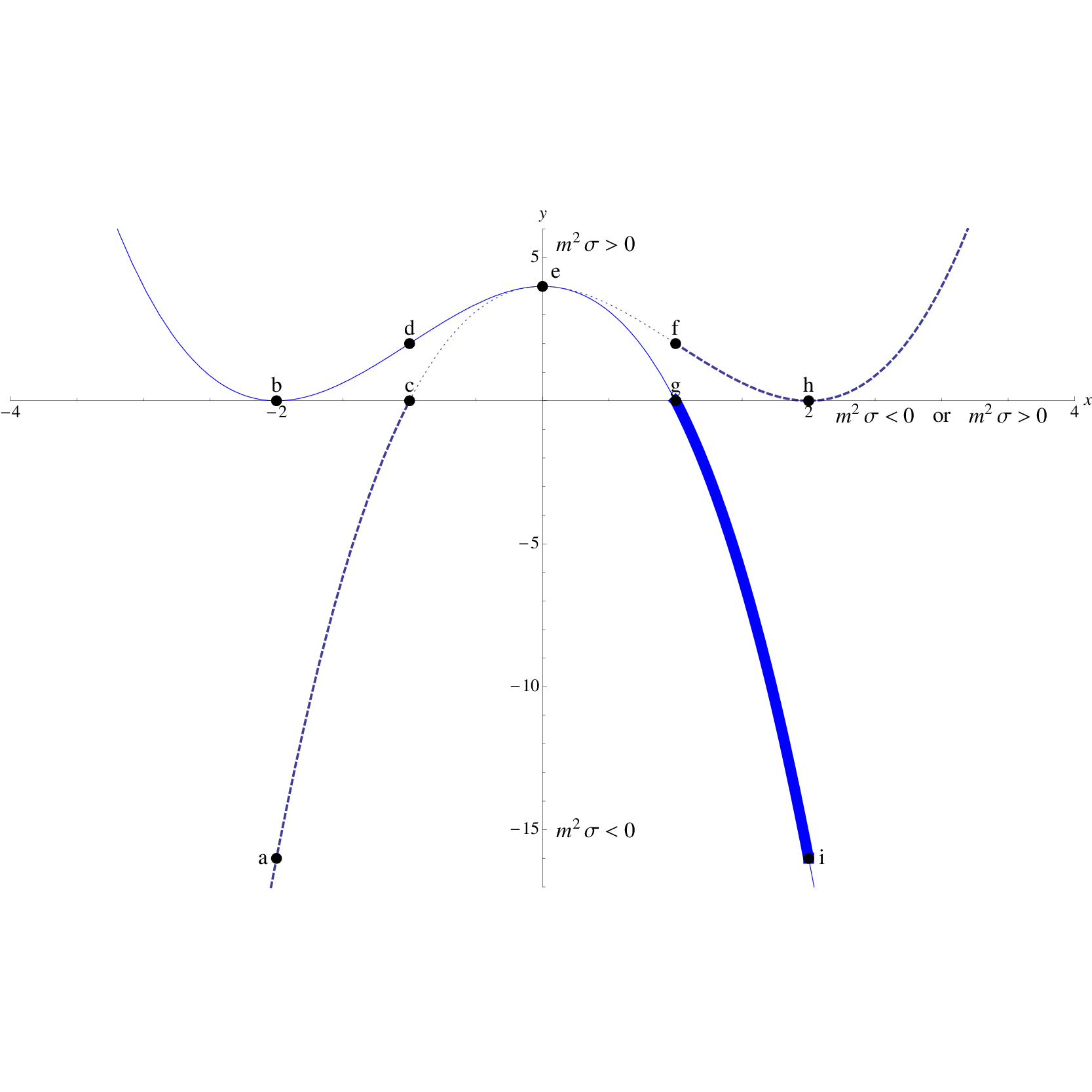
All maximally-symmetric vacua correspond to points in the $(x,y)$ -plane that lie on one of the two cubic curves

y=4-3x^{2}\mp x^{3}\,,

(4.20)

where the upper sign yields the supersymmetric vacua. Taken together, these two cubic curves yield a figure in the $(x,y)$ plane, as shown in Fig 1. This figure is symmetric under $(x,y)\to(-x,y)$ , although this transformation exchanges a supersymmetric with a non-supersymmetric vacuum, except at the fixed point $(x,y)=(0,4)$ where the two cubic curves cross. This crossing point corresponds to a supersymmetric adS vacuum with $\lambda=-\sigma^{2}$ , as follows from

\lambda+\sigma^{2}=\sigma^{2}x^{2}\,.

(4.21)

This is the unique vacuum on the $y$ -axis, from which we deduce that the dS vacuum of cosmological GMG with $\lambda=-\sigma^{2}$ and $m^{2}\sigma<0$ is not a solution of super-GMG. As pointed out in [12], the adS vacuum at $\lambda=-\sigma^{2}$ and $m^{2}\sigma>0$ has very special properties; in particular it admits a class of asymptotically adS black hole solutions, with the extremal black hole solution interpolating between the adS vacuum and a Kaluza-Klein solution with ${\rm adS}_{2}\times S^{1}$ spacetime (see also [32, 31]).

Let us now consider the possible vacua on each of the two cubic curves separately. All points on the ‘supersymmetric’ cubic curve correspond to adS vacua except, of course, the point at which this curve crosses the $x$ -axis; at this point $x=1$ , so $\Lambda=0$ . This is the supersymmetric Minkowski vacuum with $M=0$ , and $\lambda=0$ , although we could consider this point as representing two vacua since it is valid for either choice of sign of $m^{2}\sigma$ . There is also a supersymmetric adS vacuum for $m^{2}\sigma>0$ when $M=0$ ; this corresponds to the point $(x,y)=(-2,0)$ at which the curve just touches the $x$ -axis. This has $\Lambda=-6m^{2}\sigma$ , and $\lambda=3\sigma^{2}$ .

The analogous analysis for points on the ‘non-supersymmetric’ cubic curve is a little more complex. Points on this curve with $|x|>1$ correspond to dS vacua, either with $m^{2}\sigma>0$ (for $y>0$ ) or $m^{2}\sigma<0$ (for $y<0$ ). The limiting point $(x,y)=(1,2)$ corresponds to a non-supersymmetric Minkowski vacuum with $m^{2}\sigma>0$ and $\lambda=0$ . The other limiting point $(x,y)=(-1,0)$ corresponds to a dS vacuum with $m^{2}\sigma<0$ and $\lambda=0$ if it is approached from the $y<0$ side. However, it can also be approached from the $y>0$ side, in which case it corresponds to an adS vacuum with $m^{2}\sigma>0$ and $\lambda=0$ . Elsewhere on this cubic curve, i.e. for $y>0$ and $x<1$ , points on the curve correspond to adS vacua that are not supersymmetric except at the crossing point $(x,y)=(0,4)$ .

To make contact with the analysis in [12] of the maximally-symmetric vacua of GMG, we first recall that (1.4) has the solution

\Lambda=-2m^{2}\left[\sigma\pm\sqrt{\sigma^{2}+\lambda}\right]\,,

(4.22)

which shows that there are two possible vacua for each $\lambda>-\sigma^{2}$ . However, this becomes 4 vacua for each $\lambda$ if one allows either sign of $m^{2}\sigma$ . This result is manifest from Fig. 1 since each value of $\lambda>-\sigma^{2}$ corresponds to two (vertical) lines in the $(x,y)$ plane that are parallel to, but not coincident with, the $y$ -axis, and each of these vertical lines cuts each of the two cubics curves once. Actually, this is not quite right for $\lambda=0$ , but let us postpone consideration of this special case, and illustrate the generic case with $\lambda=3\sigma^{2}$ , which corresponds to $x=\pm 2$ . The choice $x=2$ yields a non-supersymmetric dS vacuum at $(x,y)=(2,0)$ (and hence $\Lambda=2m^{2}\sigma>0$ and $M=0$ ) and a supersymmetric adS vacuum at $(x,y)=(2,-16)$ (and hence $\Lambda=2m^{2}\sigma<0$ and $M\neq 0$ ). As shown in [12], the latter vacuum has very special properties; in particular, linearization about it yields a quadratic model describing massive particles of spin 1 rather than spin 2. The other choice $x=-2$ yields a supersymmetric adS vacuum at $(x,y)=(-2,0)$ (and hence $\Lambda=-6m^{2}\sigma<0$ and $M=0$ ) and a dS vacuum at $(x,y)=(-2,-16)$ (and hence $\Lambda=-6m^{2}\sigma>0$ and $M\neq 0$ ). There is complete agreement with [12] and we now learn that the two adS vacua are supersymmetric in the context of GMG.

The $\lambda=0$ case, which corresponds to $|x|=1$ , is special because the point $(x,y)=(-1,0)$ represents two possible non-supersymmetric vacua, either dS or adS, depending on the sign of $m^{2}\sigma$ , as we already observed above, and the same can be said of the point $(x,y)=(1,0)$ although both vacua are Minkowski. Taking this into account, we have six vacua for $\lambda=0$ . One may ask how this is compatible with our earlier conclusion that each value of $\lambda>-\sigma^{2}$ corresponds to four distinct vacua, allowing for either sign of $m^{2}\sigma$ . The answer to this question is that two vacua may be equivalent in the context of GMG but distinct in the context of super-GMG. For example, in the GMG context the adS vacuum at $(x,y)=(-1,2)$ would have to be considered equivalent to the adS vacuum at $(x,y)=(-1,0)$ because both have the same value of $\Lambda$ and $\lambda$ . But these two vacua have different values of $M^{2}$ in the super-GMG context; moreover, one is supersymmetric and the other is not. Similarly, the Minkowski vacuum at $(x,y)=(1,2)$ is equivalent to the $m^{2}\sigma>0$ Minkowski vacuum at $(x,y)=(1,0)$ in the GMG context, but they differ as vacua of super-GMG because they again have different values of $M^{2}$ and one is supersymmetric and the other not.

4.1.2 Other solutions

Let us now turn to solutions of super-GMG that are not maximally symmetric. Of particular interest are solutions that preserve some fraction of the supersymmetry of a supersymmetric vacuum solution; this fraction is necessarily either $1/2$ or $1$ . Let us begin with the observation that since $S=\bar{S}$ , a constant, in any solution of super-GMG (in contrast to the general model) all supersymmetric solutions have

R=-6\bar{S}^{2}\,.

(4.23)

Using this to eliminate $R$ from (4.12), we deduce that

K=-\frac{1}{24}R^{2}=-\frac{3}{2}\bar{S}^{4}\,.

(4.24)

In other words, both $R$ and $K$ must be constants, such that the vacuum relation (4.24) holds. This is a very strong condition that eliminates some otherwise plausible candidate solutions.

For example, for the special case of $\lambda=-1$ and $m^{2}\sigma>0$ , for which there is a unique adS vacuum, there is also an ${\rm adS}_{2}\times S^{1}$ ‘Kaluza-Klein’ vacuum [31]. In this vacuum

R=-4m^{2}\sigma\,,\qquad K=2m^{4}\sigma^{2}\,.

(4.25)

Since the relation (4.24) does not hold, this vacuum is not supersymmetric. It follows immediately that the static extreme black hole that interpolates between the adS vacuum (at infinity) and the ‘Kaluza-Klein’ vacuum (near the horizon) [12] is also not supersymmetric.

GMG has extremal BTZ black holes that are supersymmetric solutions of super-GMG. This is because, firstly, the BTZ black holes are isometric to an adS vacuum and hence solutions of super-GMG (because all adS vacua of GMG are solutions) and, secondly, because the analysis of whether global identifications of adS preserve some fraction of supersymmetry is independent of the choice of action. This argument actually applies to the general curvature-squared model, but we concentrate on super-GMG. Are there any other supersymmetric black holes?

To be supersymmetric a black hole must have zero Hawking temperature. This immediately excludes the class of stationary black hole solutions of NMG found in [31]. It does not exclude the class found in [33], which all have zero Hawking temperature, but we have not attempted to determine whether any of these are supersymmetric; it would be a surprise if they were given the absence of non-BTZ supersymmetric static black holes.

4.2 Generalized super-GMG

We turn now to the more general models for which $S$ is auxiliary. Given only the condition (4.1), the bosonic truncation of the general action (3.3) is

	$\displaystyle I[g,S]$	$\displaystyle=$	$\displaystyle\frac{1}{\kappa^{2}}\,\int d^{3}x\,\left\{e\left[\left(MS-2\sigma S^{2}+\frac{S^{3}}{\check{\mu}}-\frac{3S^{4}}{2(m^{\prime})^{2}}\right)+\sigma R+\frac{1}{m^{2}}K\right.\right.$		(4.26)
			$\displaystyle\left.\left.\qquad\qquad+\ \frac{1}{2\check{\mu}}RS-\frac{1}{2(m^{\prime}{}^{\prime})^{2}}RS^{2}\right]+\frac{1}{\mu}{\cal L}_{LCS}\right\}\,,$		(4.26)

where $m^{\prime}$ and $m^{\prime}{}^{\prime}$ are as defined in (3.8). The $S$ -equation of motion is algebraic:

M-4\sigma S+\frac{3S^{2}}{\check{\mu}}-\frac{6S^{3}}{(m^{\prime})^{2}}=\left(\frac{S}{(m^{\prime}{}^{\prime})^{2}}-\frac{1}{2\check{\mu}}\right)R\,,

(4.27)

and it can be solved as a power series in $R$ as long as

0\neq A\equiv 2\sigma-\frac{3\bar{S}}{\check{\mu}}+\frac{9\bar{S}^{2}}{(m^{\prime})^{2}}\,.

(4.28)

To see this, we set

S=\bar{S}+\alpha R+\frac{1}{2}\beta R^{2}+{\cal O}\left(R^{3}\right)\,,

(4.29)

where $\bar{S}$ is a constant solution of the cubic equation

M-4\sigma\bar{S}+\frac{3\bar{S}^{2}}{\check{\mu}}-\frac{6\bar{S}^{3}}{(m^{\prime})^{2}}=0\,.

(4.30)

Substitution into (4.27) yields

\alpha=\frac{1}{2A}\left(\frac{1}{2\check{\mu}}-\frac{S}{(m^{\prime}{}^{\prime})^{2}}\right)\,,\qquad\beta=\frac{\alpha}{A}\left[3\alpha\left(\frac{1}{\check{\mu}}-\frac{6\bar{S}}{(m^{\prime})^{2}}\right)-\frac{1}{(m^{\prime}{}^{\prime})^{2}}\right]\,.

(4.31)

There is no solution of the assumed form if $A=0$ ; in this case the series must involve fractional powers of $R$ . Assuming $A\neq 0$ , elimination of $S$ yields a Lagrangian density of the form

{\cal L}=e\left[-2\bar{\lambda}m^{2}+\bar{\sigma}R+\frac{1}{m^{2}}K\right]+\left(\frac{1}{2\check{\mu}}-\frac{\bar{S}}{(m^{\prime}{}^{\prime})^{2}}\right)^{2}\frac{R^{2}}{4A}+{\cal O}\left(R^{3}\right)+\frac{1}{\mu}{\cal L}_{LCS}\,,

(4.32)

where

-2\bar{\lambda}m^{2}=M\bar{S}-2\sigma\bar{S}^{2}+\frac{\bar{S}^{3}}{\check{\mu}}-\frac{3\bar{S}^{4}}{2(m^{\prime})^{2}}\,,\qquad\bar{\sigma}=\sigma+\frac{\bar{S}}{2}\left(\frac{1}{\check{\mu}}-\frac{\bar{S}}{(m^{\prime}{}^{\prime})^{2}}\right)\,.

(4.33)

We now have a model that involves, generically, an additional $R^{2}$ term as compared with GMG, as well as higher powers of $R$ . This leads to a loss of perturbative unitarity in a Minkowski vacuum and we shall see in the following section that the same is true for an adS vacuum. However, the additional $R^{2}$ term in the action is absent in the special case that

\frac{1}{2\check{\mu}}=\frac{\bar{S}}{(m^{\prime}{}^{\prime})^{2}}\,,

(4.34)

and it is then obvious from (4.27) that all higher powers of $R$ are also absent. The Lagrangian density (4.32) is therefore precisely of GMG form in this case, with coefficients

-2\bar{\lambda}m^{2}=M\bar{S}-2\sigma\bar{S}^{2}-\frac{3\bar{S}^{4}}{2(m^{\prime})^{2}}+\frac{2\bar{S}^{4}}{(m^{\prime}{}^{\prime})^{2}}\,,\qquad\bar{\sigma}=\sigma+\frac{\bar{S}^{2}}{2(m^{\prime}{}^{\prime})^{2}}\,.

(4.35)

For the analysis of the following section, it is convenient to introduce the new dimensionless parameter

a=2m^{2}\ell\left(\frac{\bar{S}}{\left(m^{\prime}{}^{\prime}\right)^{2}}-\frac{1}{\check{\mu}}\right)

(4.36)

The condition (4.34) can then be written more simply as $a=0$ . This condition defines what we shall call the “generalized super-GMG” case. We say “case” rather than “model” because the condition (4.34) is not just a relation between the parameters of the general ‘auxiliary- $S$ ’ model but also involves $\bar{S}$ .

Observe that one way to achieve $a=0$ is to set $(m^{\prime}{}^{\prime})^{2}=\infty$ and $|\check{\mu}|=\infty$ . We can view this as the special case in which both $a=0$ and $|\check{\mu}|=\infty$ since these two conditions imply $(m^{\prime}{}^{\prime})^{2}=\infty$ . What is special about it is that no condition is imposed on $\bar{S}$ , so we have a relation between the parameters of the general ‘auxiliary- $S$ ’ model that define a subclass of models. This is precisely the “super-GMG” subclass, which therefore arises as the $|\check{\mu}|=\infty$ subcase of the $a=0$ “generalized super-GMG” case. Except for this special subcase, $\bar{S}$ is constrained by the relation

\bar{S}=(m^{\prime}{}^{\prime})^{2}/2\check{\mu}\,.

(4.37)

Consistency with (4.30) then requires that

\check{\mu}M=(m^{\prime}{}^{\prime})^{2}\left(2\sigma-\frac{(m^{\prime}{}^{\prime})^{4}}{20\check{\mu}^{2}\check{m}^{2}}\right)\,.

(4.38)

If the various mass parameters of the model defined by (4.26) satisfy this equation then there exists a (constant) solution $\bar{S}$ of the equation for $S$ for which $I[g,\bar{S}]$ is a GMG action. One simple way in which this condition on the parameters can be satisfied is to take $\check{m}^{2}=\infty$ and $\check{\mu}M=2\sigma m^{2}$ .

5 Perturbative unitarity of generalized super-NMG

We now turn to the issue of linearized perturbations about supersymmetric adS vacua. One of our purposes is to make contact with the results of [12] on linearized perturbations of NMG about adS vacua. The auxiliary tensor field method used there was covariant, off-shell, and led to complete results that were easy to interpret. Here we show how this method applies to super-NMG, and extend it to deal with the generalized super-NMG case. However, we take as our starting point the generic parity-preserving ‘auxiliary- $S$ ’ model for which the Lagrangian density is obtained by taking the $|\mu|\to\infty$ in (4.26):

{\cal L}=e\left[\left(MS-2\sigma S^{2}+\frac{S^{3}}{\check{\mu}}-\frac{3S^{4}}{2(m^{\prime})^{2}}\right)+\sigma R+\frac{RS}{2\check{\mu}}-\frac{RS^{2}}{2(m^{\prime}{}^{\prime})^{2}}+\frac{1}{m^{2}}K\right]\,.

(5.1)

As explained in the previous section, elimination of $S$ leads generically to an infinite series in powers of $R$ . As each term could contribute to the quadratic approximation in an expansion about an adS vacuum, it is simpler to retain $S$ as an independent field for the purposes of computing the quadratic action. It is also simpler to replace the curvature-squared term $K$ by an equivalent Lagrangian involving an auxiliary symmetric tensor field $f_{\mu\nu}$ [5]; the resulting action is

	$\displaystyle I[g,f,S]$	$\displaystyle=$	$\displaystyle\frac{1}{\kappa^{2}}\int d^{3}x\,e\left[\left(MS-2\sigma S^{2}+\frac{S^{3}}{\check{\mu}}-\frac{3S^{4}}{2(m^{\prime})^{2}}\right)+\sigma R+\frac{RS}{2\check{\mu}}-\frac{RS^{2}}{2(m^{\prime}{}^{\prime})^{2}}\right.$		(5.2)
			$\displaystyle\left.\qquad\qquad+\ f_{\mu\nu}G^{\mu\nu}-\frac{1}{2}m^{2}g^{\mu\nu}g^{\rho\sigma}f_{\mu[\rho}f_{\nu]\sigma}\right]\,.$		(5.2)

We wish to find the quadratic approximation to this action in a supersymmetric adS vacuum with cosmological constant $\Lambda=-1/\ell^{2}$ .

5.1 Quadratic approximation

We now set

	$\displaystyle g_{\mu\nu}$	$\displaystyle=$	$\displaystyle\bar{g}_{\mu\nu}+\kappa h_{\mu\nu}\,,\qquad S\ =\ \pm\ell^{-1}+\kappa s\,,$
	$\displaystyle f_{\mu\nu}$	$\displaystyle=$	$\displaystyle-\frac{1}{\ell^{2}m^{2}}\left[\bar{g}_{\mu\nu}+\kappa h_{\mu\nu}+\ell^{2}\kappa k_{\mu\nu}\right]\,,$		(5.3)

where $h_{\mu\nu}$ , $k_{\mu\nu}$ and $s$ are independent fluctuation fields⁷⁷ 7 The mass dimensions of these fluctuation fields are: $[h]=\frac{1}{2}$ , $[s]=\frac{3}{2}$ and $[k]=\frac{5}{2}$ ., and $\bar{g}_{\mu\nu}$ is the background adS metric. We shall use the notation $\bar{D}$ to indicate a covariant derivative with respect to the standard Levi-Civita connection for the background metric. Expanding the full Ricci tensor about the adS background we find that

R_{\mu\nu}\ =\ -2\ell^{-2}\bar{g}_{\mu\nu}+\kappa R_{\mu\nu}^{(1)}+\kappa^{2}R_{\mu\nu}^{(2)}+{\cal O}(\kappa^{3})\;,

(5.4)

where

R_{\mu\nu}^{(1)}\ =\ -\frac{1}{2}\left(\bar{D}^{2}h_{\mu\nu}-\bar{D}^{\rho}\bar{D}_{\mu}h_{\rho\nu}-\bar{D}^{\rho}\bar{D}_{\nu}h_{\rho\mu}+\bar{D}_{\mu}\bar{D}_{\nu}h\right)\;.

(5.5)

We will need only the trace of the $\kappa^{2}$ term, which is

\displaystyle\bar{g}^{\mu\nu}R_{\mu\nu}^{(2)}\ =\ \frac{1}{2}h^{\mu\nu}\left(R_{\mu\nu}^{(1)}-\tfrac{1}{2}R^{(1)}\bar{g}_{\mu\nu}\right)+\text{total derivative}\,,

(5.6)

where $R^{(1)}$ is the trace of $R_{\mu\nu}^{(1)}$ in the background metric.

At this point it is useful to recall the gauge symmetries at the linearized level and what the gauge-invariant objects are. The metric fluctuation transforms in the standard way under linearized diffeomorphisms,

\displaystyle\delta_{\xi}h_{\mu\nu}\ =\ \bar{D}_{\mu}\xi_{\nu}+\bar{D}_{\nu}\xi_{\mu}\;,

(5.7)

while $k_{\mu\nu}$ and $s$ have been defined such that they are gauge-invariant. The invariant curvature of $h_{\mu\nu}$ is given by the linearized Einstein tensor modified by the cosmological constant,

\displaystyle\begin{split}{\cal G}_{\mu\nu}(h)\ &\equiv\ G_{\mu\nu}^{(1)}(h)+\Lambda h_{\mu\nu}\\ \ &=\ R_{\mu\nu}^{(1)}-{\textstyle{\frac{1}{2}}}R^{(1)}\bar{g}_{\mu\nu}-2\Lambda h_{\mu\nu}+\Lambda h\bar{g}_{\mu\nu}\;,\end{split}

(5.8)

which is the tensor that defines the linearized field equations of pure Einstein gravity with cosmological constant.

Expanding the action about the vacuum, we find that all terms linear in the fluctuations cancel provided

\displaystyle M=\pm\frac{4\sigma}{\ell}\mp\frac{2}{5\check{m}^{2}\ell^{3}}\,,

(5.9)

which is the $S$ field equation in a supersymmetric vacuum with $\bar{S}=\pm\ell^{-1}$ ; this confirms the existence of these vacua. For the quadratic terms in the Lagrangian we find the manifestly gauge-invariant expression

	$\displaystyle L^{(2)}$	$\displaystyle=$	$\displaystyle-\frac{1}{2}\hat{\sigma}h^{\mu\nu}{\cal G}_{\mu\nu}(h)+\frac{a}{\ell m^{2}}s\bar{g}^{\mu\nu}{\cal G}_{\mu\nu}(h)-\frac{1}{m^{2}}k^{\mu\nu}{\cal G}_{\mu\nu}(h)$		(5.10)
			$\displaystyle-\frac{1}{4m^{2}}\left(k^{\mu\nu}k_{\mu\nu}-k^{2}\right)-\left(2\sigma\mp\frac{3}{\ell\check{\mu}}+\frac{6}{\ell^{2}m^{2}}-\frac{21}{5\ell^{2}\check{m}^{2}}\right)s^{2}\ ,$		(5.10)

where $a$ , the parameter defined in (4.36), is now given by

a=-m^{2}\left(\frac{\ell}{\check{\mu}}\mp\frac{2}{(m^{\prime}{}^{\prime})^{2}}\right)=m^{2}\left(-\frac{\ell}{\check{\mu}}\pm\frac{2}{m^{2}}\mp\frac{6}{5{\check{m}}^{2}}\right)\ .

(5.11)

In the present context, the condition $a=0$ yields the quadratic approximation for the “generalized super-NMG” case, and the two conditions $a=0$ and $|\check{\mu}|=\infty$ yield the quadratic approximation to super-NMG. As the analysis of propagating modes will depend crucially on whether $a$ is zero or non-zero, and as the $a=0$ case is of more relevance to “massive gravity”. The parameter $\hat{\sigma}$ introduced in (3.37) will also play a significant role in what follows; it is useful to note that this parameter may be rewritten as

\hat{\sigma}=\sigma+\frac{1}{2\ell^{2}m^{2}}\pm\frac{1}{4\ell\check{\mu}}\mp\frac{a}{4\ell^{2}m^{2}}\;.

(5.12)

Our next goal is to analyze the modes propagated by the Lagrangian (5.10). After some field redefinitions, we will be able to do this by comparison with Proca and Fierz-Pauli theory in anti de Sitter space. For the convenience of the reader, we first review this topic; one of our aims will be to determine the bounds on the masses of spin- $1$ and spin- $2$ particles in adS that are implied by the absence of tachyons.

5.2 Review of Proca and Fierz-Pauli in adS

For a vector field $A_{\mu}$ the massive Proca Lagrangian in an adS background is given by

\displaystyle{\cal L}_{\rm Proca}\ =\ -\frac{1}{4}F^{\mu\nu}F_{\mu\nu}-\frac{1}{2}{\cal M}^{2}A^{\mu}A_{\mu}\;.

(5.13)

It propagates massive spin-1 modes; in 3D this means that there are two modes, one of helicity $+1$ and one of helicity $-1$ . The existence of two modes can be seen by inspecting the field equations. Variation with respect to $A_{\mu}$ yields

\displaystyle\bar{D}^{\mu}F_{\mu\nu}-{\cal M}^{2}A_{\nu}\ =\ 0\qquad\Rightarrow\qquad\bar{D}^{\mu}A_{\mu}\ =\ 0\;,

(5.14)

where the second equation (the subsidiary condition) follows by taking the divergence of the first equation. The dynamical equation can then be written as

\displaystyle\left(\bar{D}^{2}-2\Lambda-{\cal M}^{2}\right)A_{\mu}\ =\ 0\;.

(5.15)

The subsidiary condition yields one constraint, which implies that there are in total two propagating degrees of freedom.

For a symmetric tensor field $\varphi$ and mass parameter ${\cal M}$ , the FP Lagrangian in an adS background is

L_{\rm FP}(\varphi;{\cal M}^{2})=-\frac{1}{2}\varphi^{\mu\nu}{\cal G}_{\mu\nu}(\varphi)-\frac{1}{2}{\cal M}^{2}\bar{g}^{\mu\nu}\bar{g}^{\rho\sigma}\varphi_{\mu[\rho}\varphi_{\nu]\sigma}\,.

(5.16)

For ${\cal M}^{2}\neq\Lambda$ this Lagrangian propagates, massive spin-2 modes; in 3D this means that there are two modes, one of helicity $+2$ and one of helicity $-2$ . The presence of two propagating degrees of freedom can be seen by inspecting the field equation

{\cal G}_{\mu\nu}(\varphi)+\frac{1}{2}{\cal M}^{2}\left(\varphi_{\mu\nu}-\bar{g}_{\mu\nu}\bar{\varphi}\right)\ =\ 0\,,\qquad\left(\bar{\varphi}\equiv\bar{g}^{\mu\nu}\varphi_{\mu\nu}\right).

(5.17)

Taking the divergence of this equation and using the Bianchi identity $\bar{D}^{\mu}{\cal G}_{\mu\nu}=0$ , we obtain

\bar{D}^{\mu}\varphi_{\mu\nu}-\bar{D}_{\nu}\bar{\varphi}\ =\ 0\qquad\Rightarrow\qquad\bar{D}^{\mu}\bar{D}^{\nu}\varphi_{\mu\nu}-\bar{D}^{2}\bar{\varphi}\ =\ 0\;.

(5.18)

On the other hand, taking the trace of (5.17) and using the explicit form of $R^{(1)}$ in (5.5), we get

\bar{D}^{\mu}\bar{D}^{\nu}\varphi_{\mu\nu}-\bar{D}^{2}\bar{\varphi}=2\left(\Lambda-{\cal M}^{2}\right)\bar{\varphi}\,,

(5.19)

where $\Lambda<0$ is the cosmological constant. Combining this with (5.18) we conclude that $\bar{\varphi}=0$ provided that ${\cal M}^{2}\neq\Lambda$ and hence that the symmetric tensor field $\varphi$ is subject to the subsidiary conditions

\bar{D}^{\mu}\varphi_{\mu\nu}\ =\ 0\;,\qquad\bar{\varphi}\ =\ 0\;.

(5.20)

The remaining, dynamical, equation is

\left(\bar{D}^{2}-2\Lambda-{\cal M}^{2}\right)\varphi_{\mu\nu}=0\,.

(5.21)

The subsidiary conditions impose $3+1$ constraints, so just two degrees of freedom are propagated, and these can be shown to have helicities $\pm 2$ . Observe that the specific Fierz-Pauli mass term is crucial to this result because with a different relative coefficient it would not be possible to derive (5.18), and the subsidiary condition $\bar{\varphi}=0$ , needed to eliminate scalar modes, would not be a consequence of the field equations.

In the special case of ${\cal M}^{2}=\Lambda$ , the FP field equation does not imply that $\bar{\varphi}=0$ . In this case there is a ‘hidden’ gauge invariance,

\displaystyle\delta_{\zeta}\bar{k}_{\mu\nu}\ =\ \bar{D}_{\mu}\bar{D}_{\nu}\zeta+\Lambda\bar{g}_{\mu\nu}\zeta\;,

(5.22)

with scalar gauge parameter $\zeta$ . This allows the trace $\bar{\varphi}$ to be set to zero by a gauge-fixing condition. Theories of this type are known as partially massless [34, 35], and in 3D they propagate a single mode without a well-defined helicity.

There is obviously a need for some lower bound on ${\cal M}^{2}$ , in order to avoid tachyons. Let us consider the generalization of (5.21) to arbitrary integer spin $|s|$ [36]

\left[\bar{D}^{2}+|s|\left(3-|s|\right)-\mathscr{M}^{2}\right]\varphi^{(s)}=0\ ,

(5.23)

where $\varphi^{(s)}$ denotes a traceless totally symmetric rank- $|s|$ tensor satisfying the ‘divergence-free’ condition $\bar{D}^{\mu}\varphi^{(s)}_{\mu\nu_{1}\dots\nu_{s-1}}=0$ . For $|s|>0$ , the action from which this field equation is derived is gauge invariant when $\mathscr{M}^{2}=0$ . Expanding the field $\varphi^{(s)}$ in terms of the unitary irreducible representations (UIRs) of the adS₃ isometry group $Sl(2;\hbox{\mybb R})\times Sl(2;\hbox{\mybb R})$ , we find [37]

{\bar{D}}^{2}\varphi^{(s)}=E_{0}(E_{0}-2)-|s|\ ,

(5.24)

where $(E_{0},s)$ denotes the lowest weight UIR with lowest energy $E_{0}$ and helicity $s$ . These UIRs are nonsingular at the origin and normalizable with respect to the $SO(2,2)$ invariant measure [38, 39]. Using the above formula in (5.23), we find

\mathscr{M}^{2}=\left(E_{0}-|s|\right)(E_{0}+|s|-2)\ .

(5.25)

Now, it is well known that the unitarity of the representation with lowest weight $(E_{0},s)$ is given by [40]

E_{0}\geq|s|\ .

(5.26)

For $s=0$ we deduce that $\mathscr{M}^{2}\geq-1$ , which is the 3D version of the 4D Breitenlohner-Freedman bound [39, 41, 42]. For $s\geq 1$ we deduce that $\mathscr{M}^{2}\geq 0$ , as claimed for $s=1,2$ .

5.3 Diagonalization

We are now ready to continue with our analysis of the quadratic Lagrangian (5.10). The results depend crucially on whether the parameter $a$ , defined in (5.11), is zero or non-zero, so we consider these cases separately.

5.3.1 $a=0$

When $a=0$ the field $s$ may be trivially eliminated and the quadratic Lagrangian (5.10) reduces to

L^{(2)}=-\frac{1}{2}\hat{\sigma}h^{\mu\nu}{\cal G}_{\mu\nu}(h)-\frac{1}{m^{2}}k^{\mu\nu}{\cal G}_{\mu\nu}(h)-\frac{1}{4m^{2}}\left(k^{\mu\nu}k_{\mu\nu}-k^{2}\right)\,,

(5.27)

where $\hat{\sigma}$ is the parameter of (5.12). This is precisely eq. (4.17) of [12] when $|\check{\mu}|=\infty$ , which corresponds to the super-NMG model; this was to be expected because super-NMG has NMG as its bosonic truncation. The only difference between super-NMG and generalized super-NMG in the context of a quadratic approximation is in the definition of the parameter $\hat{\sigma}$ . How we now proceed depends on whether or not $\hat{\sigma}$ vanishes. We shall consider these two subcases separately.

•

$\hat{\sigma}\neq 0:$ In this case we define a new symmetric tensor fluctuation field ${\bar{h}}$ by

h_{\mu\nu}\ =\ \bar{h}_{\mu\nu}-\frac{1}{m^{2}\hat{\sigma}}\,k_{\mu\nu}\ .

(5.28)

The quadratic Lagrangian then takes the diagonal form

L^{(2)}=-\frac{1}{2}\hat{\sigma}\,\bar{h}^{\mu\nu}{\cal G}_{\mu\nu}(\bar{h})-\frac{1}{m^{4}\hat{\sigma}}\,L_{\rm FP}(k;-m^{2}\hat{\sigma})\,,

(5.29)

where $L_{\mathrm{FP}}$ was defined in (5.16). We see from this result that $\hat{\sigma}$ has the interpretation as the effective EH coefficient in a non-Minkowski vacuum. Because this term propagates no modes, we effectively have an FP Lagrangian with ${\cal M}^{2}=-m^{2}\hat{\sigma}$ . As we explained earlier, the absence of tachyons requires $\mathscr{M}^{2}\geq 0$ (which is a stronger condition that used in [12]) and hence $m^{2}\hat{\sigma}<0$ . We also require $\hat{\sigma}<0$ for positive kinetic energy (no ghosts) so we deduce that the combined conditions for no ghosts and no tachyons are

m^{2}>0\,,\qquad\sigma+\frac{1}{2\ell^{2}m^{2}}\pm\frac{1}{4\ell\check{\mu}}<0\;.

(5.30)

Note that these conditions imply that $\sigma<0$ in the NMG limit $|\check{\mu}|\to\infty$ , but $\sigma>0$ is possible in the “generalized” case.

We should recall here that the case ${\cal M}^{2}=\Lambda$ is special because it corresponds to a partially massless mode [35]. It is not clear to us whether our earlier conclusion that $\mathscr{M}^{2}\geq 0$ is required for the absence of tachyons also applies in this special case.

•

$\hat{\sigma}=0:$

In this special case, we see from (5.27) that the fluctuation field $h_{\mu\nu}$ is a Lagrange multiplier; the constraint it imposes has the general solution

$k_{\mu\nu}=2\bar{D}_{(\mu}A_{\nu)}\,,$ (5.31)

for arbitrary vector field $A_{\mu}$ . Using this solution we arrive at the equivalent Lagrangian

$L^{(2)}=-\frac{1}{4m^{2}}F^{\mu\nu}F_{\mu\nu}-\frac{2}{\ell^{2}m^{2}}A^{\mu}A_{\mu}\,,$ (5.32)

where we have discarded a total derivative. This is a Proca Lagrangian for $A_{\mu}$ , with positive kinetic energy provided $m^{2}>0$ and a specific value for the mass.

Alternatively, the Proca equations may be deduced from the equations of motion of (5.27). The $k$ field equation is

$\mathscr{G}_{\mu\nu}(h)+\frac{1}{2}\left(k_{\mu\nu}-k\bar{g}_{\mu\nu}\right)=0\,.$ (5.33)

When combined with the Bianchi identity $\bar{D}^{\mu}{\cal G}_{\mu\nu}=0$ and the $h$ field equation (5.31), this implies the Proca equations that follow from (5.32). Provided $m^{2}>0$ these equations propagate non-tachyonic modes of helicity $\pm 1$ . This is consistent with the corresponding result for NMG [12]; however, whereas $\hat{\sigma}=0$ was there found to imply $\sigma<0$ , this is not true in the “generalized” case since it follows from (5.12) that $\hat{\sigma}=0$ and $a=0$ imply

$\sigma=-\frac{1}{2\ell^{2}m^{2}}\mp\frac{1}{4\ell\check{\mu}}\ ,$ (5.34)

and this allows $\sigma<0$ when $\check{\mu}$ is finite.

Finally, we remark that the equation (5.33) does not propagate any modes if one adopts the standard Brown-Henneaux boundary conditions for the metric [10] but weaker boundary conditions allow well known logarithmic bulk modes [43]. It may be verified that the Proca modes mentioned above are mapped by (5.31) into the first descendants of the logarithmic modes; see [44] for a detailed description of precisely such a descendant mode.

The occurrence of different formulations at the linearized level is similar to what happens in TMG, in which case there exists a map of the linearized field equation at the chiral point to that of a topologically massive photon [45]. Alternatively, the linearized theory can be mapped, non-covariantly, to a scalar field satisfying the Breitenlohner-Freedman bound [46]. The linearized solution of these equations are related to the logarithmic solutions of the metric formulation, as has been shown in [46] for the scalar parametrization.

5.3.2 $a\neq 0$

When $a\neq 0$ we must return to the quadratic Lagrangian (5.10). Again we must distinguish between the $\hat{\sigma}\neq 0$ and the $\hat{\sigma}=0$ cases, so we consider them in turn.

•

$\hat{\sigma}\neq 0:$ When $\hat{\sigma}\neq 0$ the Lagrangian becomes diagonal in terms of the new symmetric tensor fluctuation fields $(\bar{h},\bar{k})$ , defined by

h_{\mu\nu}\ =\ \bar{h}_{\mu\nu}-\frac{1}{m^{2}\hat{\sigma}}\,\bar{k}_{\mu\nu}\;,\qquad k_{\mu\nu}\ =\ \bar{k}_{\mu\nu}+a\ell^{-1}s\,\bar{g}_{\mu\nu}\;,

(5.35)

where $a$ is the mass parameter defined in (5.11). The quadratic Lagrangian then takes the form

L^{(2)}=-\frac{1}{2}\hat{\sigma}\,\bar{h}^{\mu\nu}{\cal G}_{\mu\nu}(\bar{h})-\frac{1}{m^{4}\hat{\sigma}}\,L_{\rm FP}(\bar{k};-m^{2}\hat{\sigma})+\frac{a}{\ell m^{2}}\bar{k}s-bs^{2}\;,

(5.36)

where

b=\frac{1}{2}\hat{\sigma}-\frac{\left(3a\mp 2\right)\left(a\mp 2\right)}{2\ell^{2}m^{2}}\,.

(5.37)

If $b\neq 0$ then $s$ may be trivially eliminated; this will give rise to an additional $\bar{k}^{2}$ mass term which will lead to a non-unitary theory (since the specific FP mass term is crucial for unitarity).

If $b=0$ then the field $s$ becomes a Lagrange multiplier for the constraint $\bar{k}=0$ , which is one of the subsidiary conditions of the FP equations. However, the $\bar{k}_{\mu\nu}$ field equation now reads

{\cal G}_{\mu\nu}(\bar{k})=m^{2}\hat{\sigma}\left({\textstyle{\frac{1}{2}}}\bar{k}_{\mu\nu}-a\ell^{-1}s\,\bar{g}_{\mu\nu}\right)\;.

(5.38)

Taking the divergence we deduce that

\bar{D}^{\mu}\bar{k}_{\mu\nu}=2a\ell^{-1}\partial_{\nu}s\quad\Rightarrow\quad\bar{D}^{\mu}\bar{D}^{\nu}\bar{k}_{\mu\nu}=2a\ell^{-1}\bar{D}^{2}s\,.

(5.39)

Taking the trace, one finds

\bar{D}^{\mu}\bar{D}^{\nu}\bar{k}_{\mu\nu}=6\ell^{-1}m^{2}\hat{\sigma}as\;,

(5.40)

and in combination with (5.39) this gives

\left(\bar{D}^{2}-3m^{2}\hat{\sigma}\right)s=0\,.

(5.41)

In other words, the fluctuation $s$ about the vacuum value of $S$ is now a propagating mode! Whether the theory is ghost-free in presence of this mode, however, remains to be investigated.

The fact that the ‘auxiliary’ field propagates is surprising in view of the fact that the field equation for $S$ is algebraic, a cubic equation in fact, but the coefficients of this cubic equation are not constants when $a\neq 0$ . We earlier argued that one may solve for $S$ as a power series in $R$ in this case, but all orders of this series are relevant to an expansion about adS, so it is not guaranteed that the solutions for fluctuations of $S$ will be local functions of the coefficients. We now see that an ‘auxiliary $S$ ’, in the generalized sense that we have permitted in this section, is not equivalent to ‘non-propagating $S$ ’.

•

$\hat{\sigma}=0:$ Setting $\hat{\sigma}=0$ in the Lagrangian (5.10), but now allowing for $a\neq 0$ , we find that the fluctuation field $h_{\mu\nu}$ becomes a Lagrange multiplier, as before. The constraint it imposes has the general solution

k_{\mu\nu}=a\ell^{-1}s{\bar{g}}_{\mu\nu}+2\bar{D}_{(\mu}A_{\nu)}\,,

(5.42)

for arbitrary vector field $A_{\mu}$ . Using this solution we arrive at the equivalent Lagrangian

L^{(2)}=-\frac{1}{4m^{2}}F^{\mu\nu}F_{\mu\nu}-\frac{2}{\ell^{2}m^{2}}A^{\mu}A_{\mu}+\frac{2a}{\ell m^{2}}s{\bar{D}}^{\mu}A_{\mu}-bs^{2}\ ,

(5.43)

where we now have

b=-\frac{\left(3a\mp 2\right)\left(a\mp 2\right)}{2\ell^{2}m^{2}}\

(5.44)

If $b\neq 0$ , then the field $s$ can be trivially eliminated, as before, and this will give rise to additional $({\bar{D}}\cdot A)^{2}$ terms which will lead to a non-unitary theory (since the standard Proca form of the action is needed for unitarity).

If $b=0$ , then the field $s$ becomes a Lagrange multiplier for the constraint $\bar{D}\cdot A=0$ , which is the Proca subsidiary condition. Furthermore, the Proca equation is now modified to

\bar{D}^{\mu}F_{\mu\nu}-4\ell^{-2}A_{\nu}=2a\ell^{-1}\partial_{\nu}s\;.

(5.45)

Taking the divergence of this equation we deduce that

\bar{D}^{2}s=0\ .

(5.46)

So the fluctuation field $s$ propagates a scalar mode. The unitarity of the model in presence of this mode remains to be investigated.

5.4 Summary

A curiosity that our analysis has uncovered is that a scalar field may be “auxiliary” in the sense of having no kinetic term but still propagate modes in a non-Minkowski vacuum if it is coupled to scalar products of propagating fields. The distinction between “auxiliary” and “non-propagating” boils down, in the cases analysed, to whether a dimensionless parameter $a$ is non-zero (the generic case) or zero (the “non-propagating” case). The latter option yields the cases that we have referred to as those of “generalized super-NMG”. The more general “auxiliary S” models, with $a\neq 0$ , propagate scalar modes and are generically non-unitary although there may be special subcases that are perturbatively unitary.

Within “generalized super-GMG” we find the “super-NMG” models. Since these have NMG as a bosonic truncation (albeit with a restricted range of the NMG parameters) we should expect agreement with the results found for NMG in [12] . We do, except for the stricter condition on perturbative unitarity that follows from the stronger bound on the spin- $2$ Fierz-Pauli mass in adS vacua that we have justified here.

We have also shown that the super-NMG results extend to “generalized super-NMG”, the only difference being that the “effective” EH coefficient $\hat{\sigma}$ now depends on an additional parameter. This allows perturbative unitarity to be made consistent with $\sigma>0$ , i.e. with “right-sign” EH term in the action. However, it should be recalled that “generalized super-NMG” is not actually a class of “models” because its definition depends on a choice of adS vacuum; in particular, the conclusion that $\sigma<0$ is needed for perturbative unitarity in Minkowski vacua is unchanged.

6 Discussion

In this paper we have completed a study of three-dimensional (3D) ${\cal N}=1$ supergravity theories with generic curvature-squared terms that was begun in [23]. That paper was titled “Massive 3D supergravity” but contact was made with the massive gravity models introduced in [5] only in the context of an expansion about Minkowski spacetime, where non-linear features are not crucial. The space of non-Minkowski vacua found in [23] had no obvious relation to the space of non-Minkowski vacua found in [5], and neither did there appear to be any supergravity model with a bosonic truncation that could be identified with a massive gravity model. As we said in the introduction, these unsatisfactory features suggest that there is some ingredient missing from the analysis of [23], and we have shown here that this is indeed the case. The supergravity results of [23] are correct but incomplete because there is an additional super-invariant involving the auxiliary scalar field $S$ of ${\cal N}=1$ supergravity that contributes to the terms with the dimension of curvature-squared terms but not to the curvature-squared terms themselves. Incorporating this invariant into a more general action allows the choice of a special case in which $S$ can be eliminated, at least classically, to yield a model that is identical to the ‘cosmological’ extension of the “general massive gravity” (GMG) model introduced in [5], and this includes as a special case the ‘cosmological’ extension of the parity-preserving “new massive gravity” (NMG) model studied in detail in [12].

Actually, it is overstating the case to say that the new results of this paper are suggested by complications for non-Minkowski found in [23] because it is far from obvious, a priori, that a higher-derivative gravity model should arise as the truncation of a supergravity model. In fact, the results of this paper confirm the contrary conclusion for generic curvature-squared models, since the supergravity extension of the generic model necessarily involves a kinetic term for the ‘auxiliary’ scalar, thus propagating a field that was not present initially. The special feature of the NMG and GMG models, already noted in [5], is that this term is absent, so that the ‘auxiliary’ field $S$ really does remain auxiliary in the sense that its field equation is algebraic, in fact cubic. However, the incomplete results of [23] led to the conclusion that this cubic equation necessarily has coefficients that are not all constant but depend upon the scalar curvature $R$ . Elimination of $S$ then leads to an additional power series in $R$ contribution to the action; in particular, it leads to an additional unwanted $R^{2}$ term. Had this been the last word on the matter, it would have encouraged the view that that massive 3D gravities are mere curiosities. Conversely, the fact that one can recover NMG or GMG as bosonic truncations of a 3D supergravity model, as shown in this paper, paves the way to a further study of extended super-GMG models and encourages the belief that these models should have a role to play in some ‘bigger picture’.

The main point of interest in the new massive gravity models such as NMG and GMG is the fact that the higher-derivative terms are consistent with unitarity, at least in the Minkowski vacuum. This result was shown in [23] to extend to the spin- $\tfrac{3}{2}$ sector of the supergravity models, as is of course implied by supersymmetry. The issue of unitarity in adS vacua was studied in detail in [12] for NMG and we have here extended this analysis to super-NMG and some variants of it that also preserve parity. As the bosonic truncation of super-NMG is equivalent to NMG after elimination of the supergravity auxiliary field $S$ , and as all adS vacua of NMG correspond to a supersymmetric adS vacuum of super-NMG, the results of [12] for linearization about an adS vacuum extend immediately to linearization of super-NMG about a supersymmetric adS vacuum; in particular, there is no need to consider the spin- $\tfrac{3}{2}$ sector because this is determined by supersymmetry in a supersymmetric vacuum.

There is one caveat: we have shown here that the Fierz-Pauli mass $\mathscr{M}$ for a spin- $2$ field in adS₃ must satisfy $\mathscr{M}^{2}\geq 0$ in order that the associated spin- $2$ particle not be a tachyon⁸⁸ 8 We presume that this result is known but there are suggestions in the literature of a “Breitenlohner-Freedman bound for spin $2$ ” that allows $\mathscr{M}^{2}\geq-1$ , as for spin zero. whereas we allowed (provisionally) for a weaker bound in [12]. This means that the range of parameters for which the linearized theory is perturbatively unitary is more restricted than stated in [12]. Another subtlety is that although super-NMG has been defined as the model as for which the bosonic truncation yields NMG after elimination of the auxiliary field $S$ , there is a larger class of models for which the field linearized equations coincide with those of NMG if the parameters are tuned to the choice of vacuum; specifically, we can tune the parameters so that the field equation for the fluctuation of $S$ is algebraic. In this way, we slightly enlarge the class of models that are perturbatively unitary in an adS vacuum. Within this larger class perturbative unitarity is consistent with either sign of the Einstein-Hilbert term provided the new parameter $\check{\mu}$ introduced in (3.3) is chosen appropriately.

Finally, we briefly consider the two-dimensional CFTs that might be holographically related to the massive gravity models above when expanded about a supersymmetric adS vacuum. Actually, we should expect a holographically dual superconformal field theory, i.e. an SCFT, but it is unclear to us how the fermions may be taken into account in a semi-classical approximation to the bulk supergravity theory, so we instead consider only the bosonic truncations. According to the Brown-Henneaux analysis, for generic adS₃ gravity theories the asymptotic symmetry group consists of two copies of the Virasoro algebra corresponding to the two-dimensional conformal symmetry [10]. Their central charges encode important information about unitarity and the entropy of BTZ black holes. In the case of parity-preserving gravity theories that contain higher powers of the curvature tensor the (left and right) central charges are given by [47, 48]

\displaystyle c_{L}=c_{R}=\frac{\ell}{2G_{3}}g_{\mu\nu}\frac{\partial{\cal L}_{3}}{\partial R_{\mu\nu}}\;.

(6.1)

In the presence of the Lorentz Chern-Simons term, we need to add the contributions $\pm 3/(2G_{3}\mu)$ to $c_{L,R}$ [49]. Taking all these considerations into account, and starting from the general model (3.1), we obtain the following values for the central charges

\displaystyle c_{L,R}\ =\ \frac{3\ell}{2G_{3}}\left(\sigma+\frac{3}{10(\check{m})^{2}\ell^{2}}\pm\frac{1}{2\check{\mu}\ell}\pm\frac{1}{\mu\ell}\right)\ \equiv\ \frac{3\ell}{2G_{3}}\left({\hat{\sigma}}\pm\frac{1}{\mu\ell}\right)\;,

(6.2)

where we used $\Lambda=-1/\ell^{2}$ . In the special case of super-GMG we have

\hat{\sigma}=\sigma+\frac{1}{2\ell^{2}m^{2}}\,,

(6.3)

and hence agreement with the results of [23]. Perhaps the most significant feature of the formula (6.2) is that $\hat{\sigma}$ is the parameter determining the sign of the effective linearized EH term in the chosen adS background, which must be negative for perturbative unitarity. This means that the difficulty encountered in all previous massive 3D gravity models, that one must choose between non-unitary gravitons or negative mass BTZ black holes, is a rather general one that is not resolved in supergravity, no matter how one adjusts the parameters.

Acknowledgments

We acknowledge helpful discussions and correspondence with Steve Carlip, Geoffrey Compère, Daniel Grumiller and Paul Howe. We also thank each others home institutions for the hospitality extended during visits. PKT is supported by an EPSRC Senior Fellowship. The research of ES is supported in part by NSF grants PHY-0555575 and PHY-0906222. The work of O.H. is supported by the DFG–The German Science Foundation and in part by funds provided by the U.S. Department of Energy (DOE) under the cooperative research agreement DE-FG02-05ER41360.

References

[1] A. Staruszkiewicz, “Gravitation Theory In Three-Dimensional Space,” Acta Phys. Polon. 24 (1963) 735.
[2] H. Leutwyler, “A (2+1)-dimensional model for the quantum theory of gravity”, Nuovo. Cim. 42A (1966) 159.
[3] S. Deser, R. Jackiw and G. ’t Hooft, “Three-Dimensional Einstein Gravity: Dynamics Of Flat Space,” Annals Phys. 152 (1984) 220.
[4] K. S. Stelle, “Renormalization Of Higher Derivative Quantum Gravity,” Phys. Rev. D 16 (1977) 953; “Classical Gravity With Higher Derivatives,” Gen. Rel. Grav. 9 (1978) 353.
[5] E. A. Bergshoeff, O. Hohm and P. K. Townsend, “Massive Gravity in Three Dimensions,” Phys. Rev. Lett. 102 (2009) 201301 [arXiv:0901.1766 [hep-th]].
[6] E. A. Bergshoeff, O. Hohm and P. K. Townsend, “On Higher Derivatives in 3D Gravity and Higher Spin Gauge Theories,” Annals Phys. 325 (2010) 1118 [arXiv:0911.3061 [hep-th]].
[7] E. Bergshoeff, O. Hohm and P. Townsend, “On massive gravitons in 2+1 dimensions,” J. Phys. Conf. Ser. 229 (2010) 012005 [arXiv:0912.2944 [hep-th]].
[8] S. Deser, R. Jackiw and S. Templeton, “Topologically massive gauge theories”, Annals Phys. 140 (1982) 372.
[9] D. G. Boulware and S. Deser, “String Generated Gravity Models,” Phys. Rev. Lett. 55 (1985) 2656.
[10] J. D. Brown and M. Henneaux, “Central Charges in the Canonical Realization of Asymptotic Symmetries: An Example from Three-Dimensional Gravity,” Commun. Math. Phys. 104 (1986) 207.
[11] J. M. Maldacena, “The large N limit of superconformal field theories and supergravity,” Adv. Theor. Math. Phys. 2 (1998) 231 [Int. J. Theor. Phys. 38 (1999) 1113] [arXiv:hep-th/9711200].
[12] E. A. Bergshoeff, O. Hohm and P. K. Townsend, “More on Massive 3D Gravity,” Phys. Rev. D 79 (2009) 124042 [arXiv:0905.1259 [hep-th]].
[13] Y. Liu and Y. W. Sun, “Consistent Boundary Conditions for New Massive Gravity in $AdS_{3}$ ,” JHEP 0905 (2009) 039 [arXiv:0903.2933 [hep-th]]; “On the Generalized Massive Gravity in $AdS_{3}$ ,” Phys. Rev. D 79, 126001 (2009) [arXiv:0904.0403 [hep-th]].
[14] D. Grumiller and O. Hohm, “AdS₃/LCFT₂ - Correlators in New Massive Gravity,” Phys. Lett. B 686 (2010) 264 [arXiv:0911.4274 [hep-th]].
[15] O. Hohm and E. Tonni, “A boundary stress tensor for higher-derivative gravity in AdS and Lifshitz backgrounds,” JHEP 1004 (2010) 093 [arXiv:1001.3598 [hep-th]].
[16] M. Alishahiha and A. Naseh, “Holographic Renormalization of New Massive Gravity,” arXiv:1005.1544 [hep-th].
[17] D. Grumiller and I. Sachs, “AdS₃/LCFT₂ – Correlators in Cosmological Topologically Massive Gravity,” JHEP 1003 (2010) 012 [arXiv:0910.5241 [hep-th]].
[18] K. Skenderis, M. Taylor and B. C. van Rees, “Topologically Massive Gravity and the AdS/CFT Correspondence,” JHEP 0909 (2009) 045 [arXiv:0906.4926 [hep-th]]; “AdS boundary conditions and the Topologically Massive Gravity/CFT correspondence,” arXiv:0909.5617 [hep-th].
[19] A. Maloney, W. Song and A. Strominger, “Chiral Gravity, Log Gravity and Extremal CFT,” Phys. Rev. D 81 (2010) 064007 [arXiv:0903.4573 [hep-th]].
[20] E. A. Bergshoeff, O. Hohm, J. Rosseel et al., “On Critical Massive (Super)Gravity in adS3,” [arXiv:1011.1153 [hep-th]].
[21] P. S. Howe and R. W. Tucker, “Local Supersymmetry In (2+1)-Dimensions. 1. Supergravity And Differential Forms,” J. Math. Phys. 19 (1978) 869; “Local Supersymmetry In (2+1)-Dimensions. 2. An Action For A Spinning Membrane,” J. Math. Phys. 19 (1978) 981.
[22] T. Uematsu, “Structure Of N=1 Conformal And Poincare Supergravity In (1+1)-Dimensions And (2+1)-Dimensions,” Z. Phys. C 29 (1985) 143; “Constraints And Actions In Two-Dimensional And Three-Dimensional N=1 Conformal Supergravity,” Z. Phys. C 32 (1986) 33.
[23] R. Andringa, E. A. Bergshoeff, M. de Roo, O. Hohm, E. Sezgin and P. K. Townsend, “Massive 3D Supergravity,” Class. Quant. Grav. 27 (2010) 025010 [arXiv:0907.4658 [hep-th]].
[24] S. Deser, “Ghost-free, finite, fourth order D=3 (alas) gravity,” Phys. Rev. Lett. 103 (2009) 101302 [arXiv:0904.4473 [hep-th]].
[25] H. Nishino and S. Rajpoot, “(Curvature)**2-terms for supergravity in three dimension,” Phys. Lett. B 639 (2006) 110 [arXiv:hep-th/0607241].
[26] S. Deser and J. H. Kay, “Topologically Massive Supergravity,” Phys. Lett. B 120 (1983) 97.
[27] S. Deser, “Cosmological Topological Supergravity,” in Quantum Theory of Gravity, ed. S.M. Christensen, (Adam Hilger 1984), pp 374-381.
[28] P. van Nieuwenhuizen, “D = 3 Conformal Supergravity And Chern-Simons Terms,” Phys. Rev. D 32 (1985) 872.
[29] S. Deser and J. Franklin, “Is BTZ a separate superselection sector of CTMG?,” Phys. Lett. B693, 609-611 (2010). arXiv:1007.2637 [hep-th].
[30] S. Deser, R. Jackiw and S. Y. Pi, “Cotton blend gravity pp waves,” Acta Phys. Polon. B 36 (2005) 27 [arXiv:gr-qc/0409011].
[31] G. Clement, “Warped AdS₃ black holes in new massive gravity,” Class. Quant. Grav. 26 (2009) 105015 [arXiv:0902.4634 [hep-th]].
[32] J. Oliva, D. Tempo and R. Troncoso, “Three-dimensional black holes, gravitational solitons, kinks and wormholes for BHT masive gravity,” JHEP 0907 (2009) 011 [arXiv:0905.1545 [hep-th]].
[33] G. Clement, “Black holes with a null Killing vector in new massive gravity in three dimensions,” Class. Quant. Grav. 26, 165002 (2009). arXiv:0905.0553 [hep-th].
[34] S. Deser and R. I. Nepomechie, “Gauge Invariance Versus Masslessness In De Sitter Space,” Annals Phys. 154 (1984) 396.
[35] S. Deser and A. Waldron, “Partial masslessness of higher spins in (A)dS,” Nucl. Phys. B 607 (2001) 577 [arXiv:hep-th/0103198].
[36] M. Bianchi, P. J. Heslop and F. Riccioni, “More on la grande bouffe,” JHEP 0508 (2005) 088 [arXiv:hep-th/0504156].
[37] S. Deger, A. Kaya, E. Sezgin and P. Sundell, “Spectrum of D = 6, N = 4b supergravity on AdS(3) x S(3),” Nucl. Phys. B 536 (1998) 110 [arXiv:hep-th/9804166].
[38] R. Raczka, N. Limic and J. Niederle, “Discrete degenerate representations of the noncompact rotation groups,”, J. Math. Phys. 7 (1966) 1861.
[39] P. Breitenlohner and D. Z. Freedman, “Stability In Gauged Extended Supergravity,” Annals Phys. 144 (1982) 249.
[40] A. O. Barut and R. Raczka, “Theory Of Group Representations And Applications,” (World Scientific, 1986).
[41] L. Mezincescu and P. K. Townsend, “Stability At A Local Maximum In Higher Dimensional Anti-De Sitter Space And Applications To Supergravity,” Annals Phys. 160 (1985) 406.
[42] A. M. Harun ar Rashid, C. Fronsdal and M. Flato, “Three D singletons and 2-D C.F.T,” Int. J. Mod. Phys. A 7 (1992) 2193.
[43] D. Grumiller and N. Johansson, “Instability in cosmological topologically massive gravity at the chiral point,” JHEP 0807 (2008) 134 [arXiv:0805.2610 [hep-th]]; S. Ertl, D. Grumiller and N. Johansson, “Erratum to ‘Instability in cosmological topologically massive gravity at the chiral point’, arXiv:0805.2610,” arXiv:0910.1706 [hep-th].
[44] G. Giribet, M. Kleban and M. Porrati, “Topologically Massive Gravity at the Chiral Point is Not Chiral,” JHEP 0810 (2008) 045[arXiv:0807.4703 [hep-th]].
[45] S. Carlip, S. Deser, A. Waldron and D. K. Wise, “Cosmological Topologically Massive Gravitons and Photons,” Class. Quant. Grav. 26 (2009) 075008 [arXiv:0803.3998 [hep-th]].
[46] S. Carlip, “Chiral Topologically Massive Gravity and Extremal B-F Scalars,” JHEP 0909 (2009) 083 [arXiv:0906.2384 [hep-th]].
[47] H. Saida and J. Soda, “Statistical entropy of BTZ black hole in higher curvature gravity,” Phys. Lett. B 471 (2000) 358 [arXiv:gr-qc/9909061].
[48] P. Kraus and F. Larsen, “Microscopic Black Hole Entropy in Theories with Higher Derivatives,” JHEP 0509 (2005) 034 [arXiv:hep-th/0506176].
[49] P. Kraus and F. Larsen, “Holographic gravitational anomalies,” JHEP 0601 (2006) 022 [arXiv:hep-th/0508218].

1 Introduction

2 3D supergravity invariants

2.1 𝒩=1{\cal N}=1 superconformal tensor calculus

2.2 A supersymmetric curvature squared action

2.3 A new supersymmetric SnS^{n} action

3 The general ‘curvature-squared’ model

3.1 Some notation

3.2 Field equations

3.3 Maximally symmetric vacua

3.4 Review of supersymmetry-preservation conditions

3.5 The pp-wave solution revisited

4 Models with auxiliary SS

4.1 Super-GMG

4.1.1 Field equations and vacua

4.1.2 Other solutions

4.2 Generalized super-GMG

5 Perturbative unitarity of generalized super-NMG

5.1 Quadratic approximation

5.2 Review of Proca and Fierz-Pauli in adS

5.3 Diagonalization

5.3.1 a=0a=0

5.3.2 a≠0a\neq 0

5.4 Summary

6 Discussion

Acknowledgments

References

2.1 ${\cal N}=1$ superconformal tensor calculus

2.3 A new supersymmetric $S^{n}$ action

4 Models with auxiliary $S$

5.3.1 $a=0$

5.3.2 $a\neq 0$