Demixing of compact polymers chains in three dimensions

When a single polymer chain with excluded volume interactions is brought into a bad solvent, the solvent molecules strongly repel those of the chain. To minimize the interface between solvent and chain molecules, the chain will collapse and expel the solvent molecules from its interior. Similarly, a few polymer chains in a very large volume of solvent will form a dilute solution of collapsed chains. In particular, the individual chains will not mix [1].

Consider now squeezing the chains together so as to form a solution in which the monomer density is finite (and the solvent density can be taken to zero). We may then ask whether different chains will mix or segregate. One would expect that the answer to this question might depend on how the number of chains scales with the size of the system.

A well-studied case is that of a polymer melt where many chains are present. If there are of the order $N^{1/2}$ chains, occupying a total volume $N$ (i.e., with an average monomer density of $N^{-1/2}$ for each chain) the so-called Flory theorem [2] is supposed to apply. According to this, the repulsive hard-core interaction between different chains is completely screened out at large distances. This implies that a single chain within the melt exhibits ideal, Gaussian behavior: its radius of gyration scales as the square root of the chain length. In particular, different chains should mix (interpenetrate) completely, as opposed to a demixing (segregation) scenario where each chain would occupy a small lump of the available space [1].

It has recently been shown by the Strasbourg group in a number of studies [3] that the Flory theorem is not quite correct. In particular, these authors have shown that the interplay between chain connectivity and the incompressibility of the melt leads to an effective repulsion between chain segments. The bond-bond correlation function, supposed to be short-range by the Flory argument, turns out to exhibit a long-range algebraic decay. A number of deviations from the ideal Flory behavior have been pointed out, and shown to be accounted for in an improved scaling theory [3] that views the chain as a hierarchical arrangement of correlation holes [1] of sub-chains on all length scales.

On the other hand, one might be interested in the situation where there is only a finite number of chains in a solution of finite monomer density. In this context, the issue of polymer mixing has recently gained renewed interest in the area of physical biology. One outstanding question is to understand the organization and segregation of chromosomes within simple bacteria, including during duplication. In particular, the bacterium Escherichia coli with a single circular chromosome in a rod-shaped cell has served as a model system. In this situation the radius of gyration of a single chain will necessarily scale as the cube root of the chain length, and there is no good reason why the Flory theory [2] and the more recent improvements of it [3] should apply. The question whether the chains will mix in that case therefore needs to be settled separately, as do the possible consequences for chromosome organization.

The behavior of a dense solution of just two polymer chains confined to a bar-shaped geometry, akin to that of a rod-shaped cell, was discussed in [4]. A simple piston model, combined with a blob-type analysis [1] (see also [5]), was used to point out the mechanisms by which demixing might occur. In the limit of large piston pressure (corresponding to maximal density) the two chains were nevertheless found to mix. In contrast with this, studies of unentangled ring polymers in concentrated solutions [7, 8] concluded that the existence of topological barriers would lead to segregation. A molecular dynamics study, using a parameter-free bead-spring polymer model of a ring polymer melt, corroborated the segregation scenario and found several structural and dynamical results in agreement with experiments on Drosophila and budding yeast chromosomes [9]. The results of [9] imply that a certain number of experimental observations could be due to generic polymer effects, and as such could be accounted for in very simple models.

In this paper, we revisit the problem of two open chains (not rings). In line with the above reductionist point of view, we do so by studying numerically a simple and very precisely defined parameter-free lattice model of a two-chain melt of unit monomer density. This model accounts fully for the constraints of maximal monomer density, and the self and mutual avoidance of the chains.

The conformations of a single maximally compact (space filling) chain can be modelled on a lattice as a Hamiltonian walk (HW). By definition, a HW is a self-avoiding walk that visits each lattice site exactly once. Upon adding further local interactions, the HW model has been proposed as a description of protein melting [6] (with bending rigidity), or of protein folding [10] (with suitable interactions among amino acids). The simplest example of the latter is the so-called HP model in which only two types of amino acids (Hydrophobic or Polar) are taken into account.

To similarly model a melt of a finite number of chains, we can use the model of Hamiltonian chains (HC) [11] in which $M$ self- and mutually avoiding walks jointly visit all lattice sites. By definition, each chain has length at least one (its two end points cannot coincide). In what follows we shall always take the underlying lattice to be simple cubic (or square, when we occasionally compare with the two-dimensional case). It seems natural to assume that the HC model correctly describes an $M$-chain polymer melt in the large-scale limit, where lattice details should be irrelevant.

The question is then whether the HC model validates, for the case of a melt consisting of only a few chains, the mixing scenario envisaged for the two-chain case in [4]. In this paper we study in detail the simplest possible case of $M=2$ identical chains of equal length, by large-scale numerical simulations. We show that, contrary to the above expectations, the chains actually phase separate. For an $L\times L\times(rL)$ lattice, with large $L$ and fixed aspect ratio $r$, the effect turns out to be quite subtle (but measurable) for $r=1$, becoming more pronounced for larger values of $r$.

Properties of self-avoiding walks are routinely studied by importance sampling schemes of the Monte Carlo (MC) type, one well-known example being the pivot algorithm [12]. Unfortunately, almost all known algorithms become useless in the fully-packed limit, as the acceptance ratio for any proposed move tends to zero. For the HW case (i.e., the HC model with $M=1$ chain) we have recently shown that an MC move proposed by Mansfield [13] can be turned into an algorithm that is both efficient (with dynamical exponent $z\simeq 0$) and provides unbiased sampling (each conformation is generated with uniform probability) [14].

The working principle of this $M=1$ algorithm is shown in Fig. 1. Choose an end point ${\bf x}$ of the HW at random, and select one of its adjacent empty links $({\bf x}{\bf y})$. Then, among the occupied links adjacent to ${\bf y}$, there is exactly one which would form part of a loop if $({\bf x}{\bf y})$ were added to the HW; call it $({\bf y}{\bf z})$. The basic move is then to change the HW by adding $({\bf x}{\bf y})$ and removing $({\bf y}{\bf z})$.

We now state the modifications necessary to deal with the case of $M=2$. For the moment we assume that the point ${\bf x}$ is in the bulk of the system; the case when it is on the boundary will be discussed later.

Let the configuration ${\cal C}$ consist of two chains, and let ${\bf x}$ be one of the four end points chosen at random. Once again, choose with uniform probability one of its adjacent empty links $({\bf x}{\bf y})$. As before, the idea will be to modify ${\cal C}$ by adding $({\bf x}{\bf y})$ and removing one other link. But before adding the link $({\bf x}{\bf y})$, the point ${\bf y}$ may be adjacent on one or two occupied links. The former happens if ${\bf y}$ is another end point, either of the same chain as ${\bf x}$ or of the other chain; in that case the choice of the link $({\bf y}{\bf z})$ to be removed is unambiguous. In the latter case (i.e., when ${\bf y}$ is adjacent on two occupied links) one must distinguish two different situations. If ${\bf y}$ is on the same chain as ${\bf x}$, one proceeds as in the $M=1$ case, making the unique choice of ${\bf z}$ that avoids the formation of a loop. And if ${\bf x}$ and ${\bf y}$ are on different chains, one choses randomly between the two possibilities for ${\bf z}$.

It remains to discuss two subtleties. First, when ${\bf x}$ and ${\bf y}$ are end points of two different chains, the move will consist in letting the first (resp. second) chain grow (resp. retract) by one monomer. In particular, it might happen that ${\bf z}$ is the other end point of the second chain. The move would then consist in letting the second chain shrink to zero, but since this is not an allowed HC configuration, we remedy the situation by leaving ${\cal C}$ unchanged. Second, when ${\bf x}$ is at the boundary of the system, it might happen that ${\bf y}$ is chosen outside the lattice. In that case as well the move is rejected, i.e., ${\cal C}$ is left unchanged.

With all these rules, and considering that an MC move takes unit time regardless of whether it leads to a change in ${\cal C}$ or not, it follows from a careful analysis that the rule of detailed balance is satisfied. As an independent numerical check, we ran the simulation on a $2\times 2\times 3$ cubic lattice until each of the $4\,204$ possible configurations [11] had been generated $\simeq 5\cdot 10^{4}$ times. We then verified that the fluctuations in the number of occurencies of each configuration was compatible with counting statistics.

Proving that the MC move is also ergodic, i.e., that any desired configuration may be reached from an initial one in a finite number of steps, unfortunately turns out to be much harder (a proof does not even exist for the $M=1$ chain case [14]).

As in [14], we therefore resort to explicit checks of ergodicity for small 2D and 3D systems. The case of a $2\times 2$ square lattice is special, since no MC move connects the two possible configurations. But for all other $L_{x}\times L_{y}$ lattices with $2\leq L_{x},L_{y}\leq 6$, we have checked that the number of different configurations generated by the MC move, starting from an initial reference configuration, coincides precisely with the exact enumeration results of [11]. In particular, precisely $17\,570\,172$ configurations are found on the $6\times 6$ lattice. We have similarly checked ergodicity on $2\times 2\times 2$, and $2\times 2\times 3$, and $2\times 3\times 3$ cubic lattices.

Assuming that ergodicity holds in general (except for the trivial $2\times 2$ square lattice), we conclude that the MC process converges towards the equilibrium distribution, i.e., that all HC configurations are sampled with uniform probability.

In the case where the point ${\bf y}$ is an internal point on the same chain as the end point ${\bf x}$, the identification of the correct edge $({\bf y}{\bf z})$ to be removed necessitates tracing out the loop formed when adding ${\bf x}{\bf y}$. So at worst, one MC move may require a time $\sim N$. Since each move changes at most two links, it is appropriate to evaluate the autocorrelation time $\tau$ (defined in terms of the link overlap with the initial configuration) in units of the number of MC moves per site. Just as in the $M=1$ case [14] we find that in those units $\tau\sim L^{z}$ is of order unity, independently of the system size. We conclude that the dynamical exponent $z\approx 0$, proving our claim that the algorithm is efficient.

Note that our algorithm provides unbiased sampling of configurations of two chains of lengths $N_{1}$ and $N_{2}$, where only $N=N_{1}+N_{2}$ is fixed. To pursue our goal—the study whether two chains of equal length mix or not—we must impose the constraint $N_{1}=N_{2}$ in an efficient way. Trial runs for $L=16$ and aspect ratios $r=1,2$ show that the probability distribution $p(\rho)$ of the length ratio $\rho=N_{1}/N$ is very close to being uniform: we have in fact $|p(\rho)-1|<0.01$ for all $\rho\in[0.02,0.98]$. It follows that a configuration with $\rho=\frac{1}{2}$ will occur on average once for each unit of $\tau$.

It is thus tempting to collect a data point whenever $\rho=\frac{1}{2}$. There is however an important caveat. Suppose that the end points of chain 1 are deeply immersed in chain 1, and same for chain 2, and that the two chains happen to be of the same length. Then all MC moves will be such that an end point ${\bf x}$ of some chain attacks a point ${\bf y}$ on the same chain, and never on the other, thus conserving the length of either chain. If data were collected whenever $\rho=\frac{1}{2}$, a lot of measurements would be made which were spaced by just one MC move, and not one unit of $\tau$. This would strongly bias the results. A better measuring protocol is to collect a data point when $\rho=\frac{1}{2}$ and require two data points to be spaced by a least one autocorrelation time. With this protocol, each data point gives an independent configuration with $\rho=\frac{1}{2}$, taken uniformly within the ensemble of chains of equal length.

To avoid transient effects due to the choice of the initial state, we discard in each run the first 100 MC moves per site, before starting the data collection. Fig. 2 shows a measurement on a rather small system obtained using this protocol. To the eye it certainly looks like the two chains interpenetrate, but obtaining a valid conclusion will require analysing the system more carefully.

According to the standard scaling theory of polymers [1], the number of HW of length $N$ is $\sim\mu^{N}N^{\gamma-1}$ for $N\gg 1$. Here $\mu$ is a lattice-dependent connective constant, and $\gamma$ a universal conformational critical exponent. Alternatively, $\gamma$ is determined by $P(x)\sim x^{2\gamma}$, where $P(x)$ is the probability distribution of the end-to-end distance in the asymptotic regime $x\ll 1$. Using this, the conformational exponent for HW has been determined numerically as $\gamma=0.94\pm 0.02$ [14]. More recently, the consistent value $\gamma=0.95\pm 0.02$ has been reported [15].

The value of $\gamma$ can be used in various ways to argue whether $M=2$ chains will phase separate or not. One simple argument goes as follows. Suppose the two chains live in a volume $V$. In the demixing scenario, each chain would occupy a volume $V/2$, and the number of configurations would scale like that of two independent HW, viz. $\left[\mu^{V/2}(V/2)^{\gamma-1}\right]^{2}\sim\mu^{V}V^{2(\gamma-1)}$. If, on the other hand, the two chains mixed, one could make the assumption (A) that one end point of either chain would be ‘close’ and hence could be connected so as to form a single HW in volume $V$. The number of configurations would then be $\mu^{V}V^{\gamma-1}$. Comparing these, we conclude that entropy should drive the chains to mix if and only if $\gamma<1$. The above numerical determinations of $\gamma$ are then in favour of the mixing scenario.

The applicability of the above argument clearly hinges on whether the assumption (A) can be considered correct. Some partial justification can be found in [11] in which the interactions of a single HW with the surface of the system was carefully analyzed. In particular, it was found that the end points possess a clear tendency to avoid lattice sites of high coordination number, i.e., they are attracted towards the surface. Since there are fewer surface sites than bulk sites, this implies an enhanced probability for end points to be close than would have been the case if they were uniformly distributed throughout the volume. Moreover, the fact that $\gamma<1$ means that end points attract one another entropically also in the bulk.

But despite of such arguments, the assumption (A) is certainly a rather weak spot in the above argument: the existence of an attraction between end points does of course not mean that they are separated by a single lattice spacing. So the above reasoning cannot be considered as conclusive. The same is true for other variant scaling arguments that we have tried out. We therefore turn to our numerical results to determine whether the two chains will mix.

We have used our MC algorithm to generate an extensive number of independent configurations for the two-chain problem on $L\times L\times(rL)$ cubic lattices with $L=16$ or $L=20$ and various aspect ratios $1\leq r\leq 10$. In the largest simulation ($L=20$ and $r=10$) each of the chains had length $\frac{r}{2}L^{3}=40\,000$ monomers and up to $1.1\cdot 10^{5}$ statistically independent configurations were generated. The boundary conditions are non-periodic (hard wall confinement) in all three lattice directions, as shown in Fig. 2.

In a first series of runs, we produced ${\cal N}_{1}\simeq 3\cdot 10^{4}$ configurations for each $r$. For each of these, the standard deviation $\sigma_{z}=\sqrt{\langle z^{2}\rangle-\langle z\rangle^{2}}$ of the $z$-coordinates of the monomers—rescaled so that $z\in[0,1]$—was computed separately for each chain, and an average value $\langle\sigma_{z}\rangle$ was extracted from the $2{\cal N}_{1}$ measures. The results for $L=16$ systems are given in the left part of Table 1. They can be compared to the result $\sigma_{z}^{0}=\frac{1}{2\sqrt{3}}\simeq 0.28868$ which would be obtained in the case of full mixing, where the mass of each chain is uniformly distributed in the $z$-direction.

The results for $\langle\sigma_{z}\rangle$ indicate that the two chains tend to demix, and that this tendency grows with increasing $r$. Of course, one is far away from the value $\frac{1}{2}\sigma_{z}^{0}$ which would result in the hypothetical situation of complete demixing, where one chain goes completely to the left of the box, and the other to the right. Note also that the difference from $\sigma_{z}^{0}$ is clearly measurable—albeit tiny—for $r=1$ where the three coordinates are equivalent.

To give more evidence for the demixing, and characterise it more precisely, we turn to a second series of runs. In this series we construct the probability density $p(\Delta z)$ of the quantity $\Delta z=|z_{1}-z_{2}|$, where $z_{i}=\langle z\rangle$ is the $z$-coordinate of the center of mass of the monomers in chain $i$ (for $i=1,2$). Obviously, constructing a whole probability distribution calls for better statistics, so in this series we produced ${\cal N}_{2}\simeq 1.1\cdot 10^{5}$ configurations for each $r$. The results for $p(\Delta z)$ are shown in Fig. 3. To eliminate fluctuations arising from the lattice discretization, the values of $\Delta z$ have been arranged into 50 ‘running’ bins; the statistical error bars can be judged from the remaining small ripples on the curves.

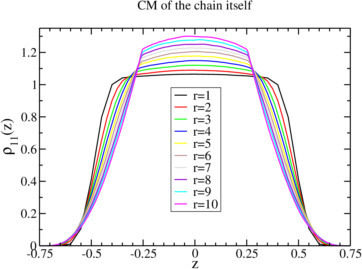
In a third series of runs we have focused on the mass density $\rho_{ij}(z)$ of chain $i$, measured relative to the center of mass $z_{j}$ of chain $j$ (for $i=1,2$). The normalization is chosen so that $\int\rho_{ij}(z)\,{\rm d}z=1$. Demixing can be detected via a different behavior for the density of a chain in its own center of mass ($\rho_{11}=\rho_{22}$ by symmetry) and for the density of a chain in the center of mass of the other chain ($\rho_{12}=\rho_{21}$). For these measurements we have taken $L=20$ and produced up to ${\cal N}_{3}\simeq 3\cdot 10^{4}$ configurations for each $r$. Instead of using bins, we have simply rounded the center of mass coordinates as expressed in lattice spacings (i.e., $rLz_{j}$) to the nearest integer. The results for $\rho_{11}(z)$ are given in Fig. 4, and those for $\rho_{12}(z)$ in Fig. 5. Both functions should of course be symmetric upon reversing the coordinate axis, $\rho_{ij}(z)=\rho_{ij}(-z)$, and the error bars can be judged from the slight deviations from this symmetry. It is seen from the figures that when $r$ increases, $\rho_{11}(z)$ tends to become a more narrow distribution around the origin, whereas $\rho_{12}(z)$ spreads out and develops a depletion near the origin. This is again clear evidence of demixing.

The data in Fig. 3 give clear evidence for demixing as $r$ increases. For small $r$ we see a rather broad distribution $p(\Delta z)$, localized around the origin. At $r\simeq 7$, the distribution becomes almost uniform, and for higher $r$ a peak near $\Delta z=\frac{1}{2}$, the maximal possible value, develops on a close-to-uniform background. To make sure that this conclusion is not a finite-size artefact, we recomputed the $r=10$ curve for a larger size $L=20$. Note that this computation required several years of CPU time. The result, shown as a dashed curve in Fig. 3, does not deviate substantially from the $L=16$ result.

It is useful to compare this situation to that of a single non-fully packed chain that is constrained to take up precisely one half of the available volume. To study this, we employ the non-fully packed version of the $M=1$ algorithm, discussed very briefly at the end of [14]. To set the peak of the monomer concentration $\rho=N/V$ precisely at $\rho=\frac{1}{2}$, one needs to tune the Boltzmann weight $w$ of a monomer. Still for $L=16$, we find that this is obtained for $w=w_{\star}$, where values of $w_{\star}$ for different $r$ are given in the right part of Table 1. This allows us to take a series of data for which each configuration has $\rho=\frac{1}{2}$ precisely. Based on a set of ${\cal N}_{3}\simeq 10^{4}$ data points, we then construct the probability distribution $p(z_{1})$ of the center of mass $z_{1}$ of the chain. For convenience, we here subtract $\frac{1}{2}$ from the $z$-coordinates so as to set the origin in the middle of the box; the support of $p(z_{1})$ is then $z_{1}\in[-\frac{1}{4},\frac{1}{4}]$. The results for $p(z_{1})$, using this time 200 bins, are given in Fig. 6.

It is of course completely predictable that these distributions are Gaussian; we find indeed $p(z_{1})\simeq a\exp\big(-b(z_{1})^{2}\big)$ with $b=(0.91\pm 0.01)\times r$. But more importantly, comparing Figs. 3–6, one can appreciate that even for $r=1$ the distribution $p(\Delta z)$ is indeed very broad. This corroborates our previous claims that even for $r=1$ the two-chain problem indeed exhibits demixing.

It is useful to compare the data in Figs. 4–5 to the hypothetical situations of complete mixing (with both chains uniformly distributed in the $z$-direction) and of complete demixing (with one chain occupying the left half of the box, $0<z<\frac{1}{2}$, and the other chain the right half, $\frac{1}{2}<z<1$). In these two extremal situations, the mass distributions $\rho_{11}(z)$ and $\rho_{12}(z)$ would be those shown in Fig. 7. The data of Figs. 4–5 bear some resemblance to a crossover (with increasing $r$) between these extremes. A closer examination of the data however indicates that for $r\gg 1$ the distributions $\rho_{ij}(z)$ will not coincide with those of the complete demixing scenario. (For instance, the tails in Fig. 4 extending out to $z=\pm\frac{3}{4}$ seem to be robust upon increasing $r$.) Note also that in terms of the distribution $p(\Delta z)$ of Fig. 3 complete demixing would correspond to a Dirac delta function $\delta(z-\frac{1}{2})$, whereas the actual data are indicative of a close-to-uniform distribution on $[0,\frac{1}{2}]$, plus possible a finite peak near $z=\frac{1}{2}$. In other words, the numerics strongly supports the idea that the physics in the limit $\lim_{r\to\infty}\lim_{L\to\infty}$ (with the thermodynamic limit being taken first) is non-trivial and corresponds to some kind of “partial demixing”.

We have studied a problem of two compact polymer chains of equal length in a three-dimensional box of various aspect ratios $r$. We have devised an efficient Monte Carlo method for sampling all configurations of this problem with uniform probability. Naive scaling theory, combined with existing evaluations of the conformational exponent $\gamma$ for a Hamiltonian walk, indicates that the two chains should mix completely. This same conclusion would be suggested by the Flory theorem [6] for a polymer melt of many chains, or from a blob-type analysis for a simple piston model of just two chains [4]. However, our numerical simulations clearly show that the two chains do in fact phase separate, even for $r=1$, and that this demixing becomes more pronounced, albeit not perfect, in the limit of large $r$.

Clearly, further work is needed to see whether this conclusion can be reconciled with some improved scaling theory, specifically adapted to a melt consisting of just a few chains. The demixing scenario obtained in this paper is somewhat subtle, since it is not due to the additive terms of the free energy. Further study is therefore required to assess whether the effect is stable towards introducing more parameters into the model (non-identical chain lengths, specific chemical interactions at the chain ends, off-lattice modelling, etc.). It would also be interesting to see whether demixing can be realized experimentally.

References

- [1] P.-G. de Gennes, Scaling concepts in polymer physics (Cornell University Press, New York, 1979).
- [2] P.J. Flory, J. Chem. Phys. 17, 303 (1949).
- [3] J.P. Wittmer et al., Phys. Rev. E 76, 011803 (2007); Phys. Rev. Lett 93, 147801 (2004); Europhys. Lett. 77, 56003 (2007).
- [4] S. Jun, Can entropy save bacteria?, arXiv:0808.2646; S. Jun and A. Wright, Nature Rev. Microbiol. 8, 600 (2010).
- [5] F. Brochard and P.-G. de Gennes, J. de Phys. Lett. (France) 40, 399 (1979).
- [6] P.J. Flory, Proc. Roy. Soc. London A 234, 60 (1956).
- [7] M. Müller, J.P. Wittmer and M.E. Cates, Phys. Rev. E 61, 4078 (2000).
- [8] S. Jun and B. Mulder, Proc. Natl. Acad. Sci. USA 103, 12388 (2006).
- [9] A. Rosa and R. Everaers, PLoS Comput. Biol. 4, e1000153 (2008).
- [10] K.A. Dill, Protein Science 8, 1166 (1999).
- [11] J.L. Jacobsen, J. Phys. A 40, 14667 (2007).
- [12] M. Lal, Molec. Phys. 17, 57 (1969); N. Madras and A.D. Sokal, J. Stat. Phys. 50, 109 (1988); B. Li, N. Madras and A.D. Sokal, J. Stat. Phys. 80, 661 (1995).
- [13] M.L. Mansfield, J. Chem. Phys. 77, 1554 (1982).
- [14] J.L. Jacobsen, Phys. Rev. Lett. 100, 118102 (2008).
- [15] M. Bohn and D.W. Heermann, J. Chem. Phys. 130, 174901 (2009).