Observable dynamics and coordinate systems for automotive target tracking
Abstract
We investigate several coordinate systems and dynamical vector fields for target tracking to be used in driver assistance systems. We show how to express the discrete dynamics of maneuvering target vehicles in arbitrary coordinates starting from the target’s and the own (ego) vehicle’s assumed dynamical model in global coordinates. We clarify the notion of “ego compensation” and show how non-inertial effects are to be included when using a body-fixed coordinate system for target tracking. We finally compare the tracking error of different combinations of target tracking coordinates and dynamical vector fields for simulated data.
I INTRODUCTION
Driver assistance systems (DAS) such as adaptive cruise control (ACC) or lane departure warning (LDW) need to perceive the environment using exteroceptive sensors (e. g. radar or laser for ACC and camera for LDW). As DAS become more sophisticated and move from comfort applications to safety-critical applications such as automatic emergency braking, the requirements regarding perception are becoming more stringent. An essential part of exteroception is the target dynamics used in the temporal prediction of observers with a predictor-corrector structure. In this paper different target dynamics in different coordinate systems will be derived and assessed with respect to satisfactory modeling of target dynamics and observability.
The modeling of target dynamics without an explicit estimation of the target driver’s intent for DAS is generally approximated by assuming non-maneuver or maneuver models [1, 2] of varying degrees of complexity [3] where the target driver’s actions like accelerating or steering are subsumed into (Gaussian) noise processes:
with the target state vector in global coordinates, the input (control) vector, and a multi-dimensional stochastic process. Those models are usually formulated with respect to a global, inertial reference frame11 1 The effect of the earth’s rotation around its polar axis as well as its rotation around the sun, etc on the vehicle motion can safely be neglected, hence an earth fixed reference frame will be called “inertial” in this paper. tangential to the earth’s surface. This also applies to the modeling of the ownship (“ego”) dynamics, however the corresponding observer can be fed with proprioceptive measurements such as yaw rate, lateral acceleration, or longitudinal velocity coming from vehicle stability control (VSC) systems. Since in both target and ego modeling the input is usually zero, we will suppress the input vectors in these vector fields from now on.
Estimation of the target dynamics is based on exteroception by radar, laser, or video sensors that provide measurements relative to the ego vehicle. Hence somewhere in the estimation process a transformation from relative to global coordinates must be performed.22 2 Modeling the target dynamics a priori in coordinates relative to the ego vehicle is rather unattractive and not considered here since e. g. a constant acceleration model for would imply that the target permanently moves with a constant acceleration plus noise relative to the ego vehicle irrespective of the actual state and motion of the ego vehicle. A dynamical system for the combined target and ego observer would then have the following form
| (1) |
where the ’s are stochastic measurement processes. Since the measurements are relative to the ego vehicle, the output function must contain a control vector in order to map the relative measurements onto the global target state . As all relative measurements contain some sort of position information, the ego state must hence also estimate the position of the ego vehicle.
This would be an appropriate approach if the ego state were fully observable which implies absolute position measurements by e. g. GPS receivers. If were not fully observable its covariance would grow without bounds which would cause the covariance matrix of to grow infinitely by propagation through the output function . This means that the dynamical system not stochastically observable – a necessary condition for the convergence of an extended Kalman filter (EKF), see e. g. [4]. Since most vehicles are not equipped with a GPS receiver, their position can only be estimated by dead-reckoning and is therefore unobservable. Even if vehicles are equipped with a GPS receiver e. g. from their navigation system, the GPS position (without differential corrections) is only accurate to about [5]. This error would then be propagated to unacceptably large position covariances in . While the covariance of the relative position in this case might remain bounded as suggested in [6] it is not advisable to work with unobservable, non-convergent systems whose ever-growing covariances will also invalidate the propagation of covariance by linearization as in an EKF.
Hence we propose formulating the target dynamics in relative, i. e. in ego vehicle fixed coordinates. The goal is to replace the combined dynamical system (1) with a system that contains and where the unobservable states of are not used for the estimation of . In the next section it will be shown how to derive the relative target dynamics starting from the global target and ego dynamics in eq. 1. While the use of relative target dynamics for automotive target tracking is not new (see e. g. [7, 8, 9]), in this paper a general, system-theoretic framework for the rigorous derivation of relative target dynamics starting from arbitrary dynamical vector fields for global target and ego dynamics is presented. This includes the derivation of the discrete dynamics with process and input noise covariance matrices as needed for an EKF as observer. The derivation is illustrated by three different choices of coordinate systems and vector fields and their accuracy in tracking targets is assessed by numerical simulation. The observability of the combined target and ego dynamics is also discussed.

II RELATIVE TARGET VEHICLE DYNAMICS
II-A Derivation
In order to derive the discrete target dynamics in relative coordinates we first need to obtain its continuous vector field. This requires a definition of the state vectors for the global target and ego dynamics and their continuous vector fields as well as a definition of the relative coordinates. The vector fields are given by
| (2) |
where we assume that no control inputs are necessary for and . We now define a new state by
| (3) |
where is in general a nonlinear function that depends upon the choice of the coordinates of , (Cartesian, polar, etc). If both and are in Cartesian coordinates and the new coordinates are also Cartesian coordinates for a ego body fixed system we get the more intuitive expression
| (4) |
where contains a rotation to the ego-fixed coordinate system as well as corrections due to the fact that the ego-fixed system is a non-inertial system and thus experiences pseudo-forces, see app. -A.33 3 From now on, we suppress the dependence of on in our notation. By taking the time derivative of eq. (4) we get a vector field for
However, the goal of this computation is to replace with ; therefore we need to use eq. (4) again in order to eliminate :
| (5) | |||||
The combined system of differential equations for and reads
| (6) |
This system of differential equations governs the dynamics of the target vehicle relative to the ego vehicle and are based upon: the dynamics of the target vehicle with respect to the ground , the dynamics of the ego vehicle with respect to the ground , and the definition of the relative coordinates . This procedure separates dynamical models for individual vehicle dynamics (ego or target) from the relative dynamics used for tracking in an arbitrary coordinate system. The “ego compensation” at the level of continuous dynamics is not a separate step but is intertwined with the relative dynamics.
II-B Solution
In this paper, all stochastic differential equations are chosen to be solved by the discrete-time counterpart method [1] where the continuous stochastic process is replaced by a discrete stochastic process which is constant from one time step to the next.44 4 Alternatively, the discrete-time equivalent method [1] can be employed using the power spectral density of the continuous stochastic process. By abuse of notation, here also denotes this constant value.
Since the ego dynamics is decoupled from the relative target dynamics, it can be solved first, see app. -B, and its solution can be inserted into the differential equation for to arrive at a time-dependent differential equation:
| (7) | |||||
The solution of this differential equation - if it exists - can be cast into the notation of discrete time systems to be used later for application of the EKF:
| (8) |
where is the time difference from one iteration to the next and is the effective discrete stochastic process for the relative target dynamics. Note that does not have inputs but has the ego state as its input or control vector.
In the following we will assume that the ego estimation using proprioceptive measurements from VSC sensors is separate from the exteroception and only outputs the ego state and its covariance matrix .
For the use of eq. (8) in an EKF, we define the matrices
which are used for the propagation of the state (), input (), and process noise () covariances by linearization. The input noise and process noise covariance matrices are then
where . Since nonlinear effects in estimation are not the focus of this paper we content ourselves in the numerical analysis with the standard EKF55 5 The local convergence of the EKF for nonlinear discrete-time systems has been proven in [4] under certain conditions. unlike in [3] where the unscented Kalman filter was used. Note however, that even the unscented transformation does not fully propagate the second moments of a multi-dimensional probability distribution [10].
II-C Vehicle dynamics
In eq. (6) arbitrary vector fields and can be used, in this paper, however, we focus on two common object dynamics, namely the white noise jerk model (see e. g. [1]) and the constant turn rate and acceleration model (CTRA, see app. -B). While the former might be advantageous in the object initialization stage if velocity and/or acceleration are not directly measured and are initialized by default values or if not just vehicles but also other objects such as pedestrians are perceived, the latter better represents the non-holonomic behavior of wheeled vehicles and also performed best in a comparative study of vehicle motion models [3]. For the ego dynamics only the CTRA model is considered in this paper.
II-D Relative coordinate systems
After choosing the target and ego dynamics the relative coordinate system for target tracking must be specified. We will investigate two different coordinate systems, one in which the entire target motion is relative to the ego vehicle (pure relative coordinates) and one in which the target position is estimated relative to the ego vehicle whereas the velocity and acceleration are estimated over ground, but rotated into the ego coordinate system (“mixed” coordinates). We will not dwell on other aspects of coordinate system choices such as the performance of polar versus Cartesian coordinates for target tracking as in [11].
III Examples
III-A Tracking in relative coordinates, white noise jerk model
For this example the global target dynamics is the non-maneuver white noise jerk model. It is naturally expressed in Cartesian coordinates, see e. g. [1]. The ego dynamics is given by the CTRA model. The relative dynamics is expressed in Cartesian coordinates. In order to apply eq. (3), the ego state vector must be transformed to Cartesian coordinates as well. With this choice the function reads
as in (4) and we obtain as in (5)
Using the ego trajectory eq. (16) and defining we obtain
with
| (9) | |||||
Note that the non-trivial components of this differential equation are - as expected - the highest derivatives; everything else is purely kinematic. This would not have been the case had we omitted the non-inertial contributions in .
In eq. (7) the target state vector is rotated into the ego coordinate system. This rotation, however, is not applied to the target process noise . On the other hand, the relative target dynamics should not depend on the orientation of an arbitrary global coordinate system. In (9) the terms proportional to and depend on the global orientation of the ego vehicle. It can be checked, however, that by choosing the process noise to be isotropic, i. e. with identical covariance values for and , the process covariance matrix becomes independent of .
This differential equation is of the form and can therefore be solved by the standard formula for linear time-invariant systems which is also valid for time-variant , see e. g. [12]. Since the solution and the corresponding Jacobians , , and are rather unwieldy expressions which can easily be computed by standard symbolic computation engines such as Matlab’s symbolic toolbox, we will not provide them here.
III-B Tracking in mixed coordinates, white noise jerk model
For this example the global target dynamics is again the non-maneuver white noise jerk model. However, in “mixed” coordinates, velocities and accelerations are the inertial quantities measured over ground, rotated into the ego coordinate system. This has the advantage that the dynamics of velocity and acceleration is reduced in the sense that the range of values of the velocity and acceleration is cut in half. This is particularly important for the object initialization of not measured states like acceleration.
Again we transform the ego state vector to Cartesian coordinates: . Then we use matrix without non-inertial terms since the velocities and accelerations are now inertial quantities and introduce a projector to project out the ego velocities and accelerations
The resulting differential equation reads
| (10) | |||||
Using the ego trajectory eq. (16) and redefining we obtain
| (11) |
As in (9), the terms proportional to and depend on the global orientation of the ego vehicle. By choosing the process noise to be isotropic the process covariance matrix again becomes independent of .
This differential equation is also of the form and can be solved by linear system techniques. Again we will not provide the unwieldy but easily computable solution.
III-C Tracking in mixed coordinates, CTRA model
Using the CTRA model for the representation of the target dynamics, it is more convenient not to transform to Cartesian coordinates. Hence both and are interpreted as . The relative coordinates are the relative and position with respect to the ego vehicle coordinate system, the angle between the ego and target velocities over ground which coincides for the CTRA models with the relative angle of the vehicle orientations, the target yaw rate over ground and the target speed and longitudinal acceleration over ground.
The coordinate transformation for this setting is
The resulting differential equation reads
Using the ego trajectory eq. (16) and defining we obtain
| (12) |
This non-linear differential equation can be solved as follows: the lower four entries of (12) can easily be solved by direct integration. Those expressions can now be inserted into the first two components. They are then of the form and can be solved by linear system techniques. Since terms proportional to appear inside the sine and cosine, integration results in Fresnel integrals. We therefore expand the integrand to first order in for analytically tractable expressions. Again, the explicit solutions are not provided for lack of space, however by setting the accelerations and as well as the process noises , , , and to zero, the state update expressions as in [9] are recovered.
IV NUMERICAL RESULTS
IV-A Simulation setup
In order to assess the estimation accuracy of the above dynamical models in different coordinate systems, a numerical study was performed. First, 50 trajectories with a duration of for the ego as well as the target vehicle were generated using the CTRA model described in app. -B. The process noise for both CTRA models was chosen to be . In order to perturb the reference trajectories away from the CTRA model, noise was added to the component. From these reference trajectories, proprioceptive and exteroceptive measurements corrupted with additive white noise are extracted every - a typical value for radar or laser measurements. Then the exteroceptive measurements are fed into three extended Kalman filters using the three discrete dynamics introduced in section III, see fig. 2. The contribution of the process noise from the ego dynamics as well as of the relative target dynamics using the CTRA in model C were set to the above values for the reference trajectory generation. The contribution of the relative target dynamics using the white noise jerk dynamics in models A and B were determined by numerically computing the values of over all 50 reference trajectories.
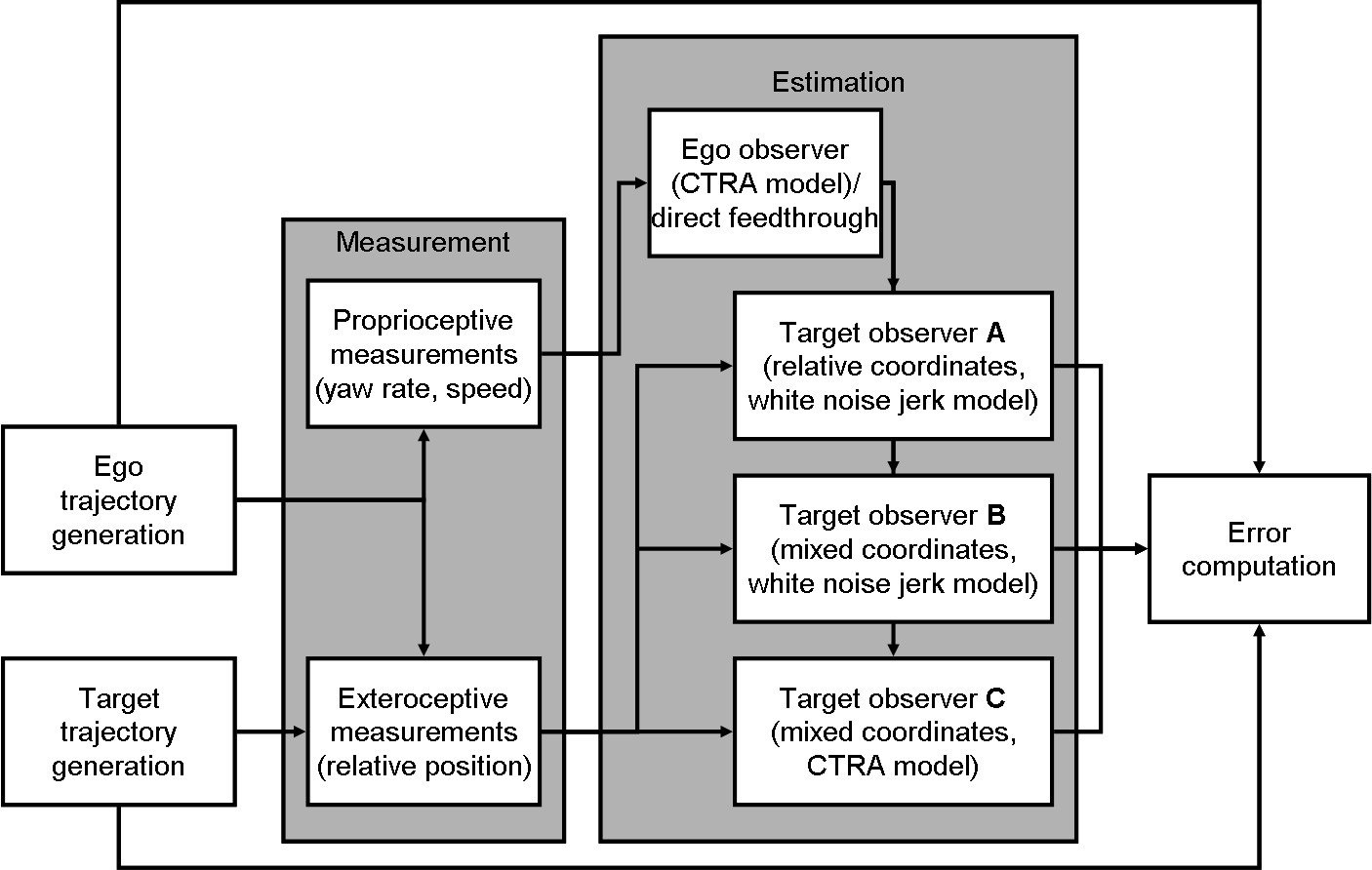
For track initialization, the not-measured entries of the state vector were set to zero. The proprioceptive measurements are fed into an EKF using the CTRA model for the estimation of the ego trajectory. The output of the proprioception serves as an input or control vector for the exteroceptive observers. Finally the Euclidean error of the position estimation with respect to the reference trajectories is determined.
IV-B Comparison of estimation errors
At every time step of every trajectory , the Euclidean error of the estimated relative position
is computed where is the rotation matrix as in eq. (13). The estimation performance is then subsumed into the average over all trajectories of the maximal error of an individual trajectory - - as well as the average over all trajectories of the mean error of an individual trajectory: .
| Model | |||
|---|---|---|---|
| A | 7.60 | 1.52 | |
| B | 4.35 | 1.02 | |
| C | 4.17 | 0.95 |
As can be seen in the first three columns of table I, the errors become smaller from model A to model C. Going from purely relative to partially relative (“mixed”) coordinates (A B) has a larger effect than going from the white noise jerk model for the target dynamics to the CTRA model in mixed coordinates (B C).
IV-C Observability analysis
In the introduction it was stated that the target state in global coordinates is unobservable if the ego vehicle has no absolute position measurements by e. g. GPS and that the target state is poorly observable if GPS-only (without differential corrections) measurements are available.
On the other hand, by formulating the target dynamics in a relative coordinate system as in section II, the target dynamics might become observable if at least relative 2d position measurements are provided by the exteroceptive sensors. As can be seen in section III, only the observable quantities , , and enter the vector fields in eqs. 9, 11, and 12.66 6 As already stated, the dependence of the process noise covariance matrix on disappears if the Cartesian process noise is chosen to be isotropic. Hence also the induced norm of the combined input and process noise is bounded – another necessary condition for the convergence of the EKF [4].
For the observability analysis we have evaluated the determinant of the observability Gramian (see e. g. [12]) over all trajectories. The determinants for models A and B are exactly ; this is also the expression for the simple 2d white noise jerk model as in [13]. The determinant for model C turned out to be too complex to be derived analytically and is given by a numerical range in table I.
As can be seen in the last column of table I models A and B are always observable irrespective of the state, whereas model C can become unobservable. This happens for example when speed and acceleration over ground become zero. However despite the intermittent ill-observability, model C performs best in terms of the estimation error (table I).
V CONCLUSIONS AND OUTLOOK
In this paper a general framework for the derivation of the dynamical vector field of the relative target dynamics for target tracking based on the vector fields for the global target and ego dynamics was presented. It was also shown how non-inertial contributions are taken into account when relative (body-fixed) velocities and accelerations are part of the state vector. The framework was applied to three different combinations of target and ego dynamics and coordinate choices and their ability in tracking targets was assessed by a numerical study. Model C, the CTRA model formulated in mixed coordinates, i. e. with relative position and angle coordinates but global (over ground) angle rate, speed, and acceleration coordinates, turned out to be more accurate than the other two models.
Since model C can become unobservable, its observability should be studied more carefully. Although a point in state space where the system becomes unobservable has already been identified, an exhaustive characterization of the unobservable state and input subspace is required along with an analysis how those unobservable subspaces affect the overall tracking performance in realistic driving scenarios.
-A 2D rotations and non-inertial contributions
The 2D rotation matrix is given by
| (13) |
The transformation of a six-dimensional vector containing the differences between target and ego vehicle in horizontal position, velocity, and acceleration over ground into body fixed coordinates is accomplished by the matrix
| (14) |
On the diagonal are the rotation matrices (13) while the off-diagonal terms are due to non-inertial corrections: e. g. the entries and give rise to centrifugal and Coriolis pseudo-forces, respectively, see e. g. [14]. The -term provides a necessary velocity correction as can be seen in fig. 3.

Without the correction term which can also be written in 3d vector notation as the relative velocity would not be zero.
-B Constant turn rate and acceleration model
A special case of a 2d curvilinear motion model [1] is here referred to as the constant turn rate and acceleration model (CTRA); its simpler version, the constant turn rate and velocity model (CTRV) represents the non-holonomic system of a vertical disk rolling on a horizontal plane [14]. Both models are commonly used to approximate a wheeled vehicle’s dynamics under normal driving conditions where the slip angle can be neglected [3]. The longitudinal acceleration is included in the state vector since e. g. ACC systems use the acceleration of the target vehicle as a control input. Its continuous dynamics is given by
| (15) |
The discrete-time counterpart solution
| (16) |
with can be obtained by linear system techniques and is not provided here for lack of space. It contains Fresnel integrals which can be expanded to first order in to obtain analytically tractable expressions. The solution also has inessential singularities at which can be removed by Taylor expansion.
References
- [1] X. Rong Li and V. Jilkov, “Survey of maneuvering target tracking. Part I. Dynamic models,” IEEE Transactions on Aerospace and Electronic Systems, vol. 39, no. 4, pp. 1333–1364, 2003.
- [2] Y. Bar-Shalom, X. Rong Li, and T. Kirubarajan, Estimation with Applications to Tracking and Navigation. Wiley, 2001.
- [3] R. Schubert, E. Richter, and G. Wanielik, “Comparison and evaluation of advanced motion models for vehicle tracking,” in Proceedings of the 11th International Conference on Information Fusion, 2008, pp. 730–735.
- [4] Y. Song and J. Grizzle, “The extended Kalman filter as a local asymptotic observer for nonlinear discrete-time systems,” Journal of Mathematical Systems, Estimation and Control, vol. 5, no. 1, pp. 59–78, 1995.
- [5] Wikipedia, “Global positioning system,” http://en.wikipedia.org/wiki/Global_Positioning_System, 2009.
- [6] M. Bühren and B. Yang, “A global motion model for target tracking in automotive applications,” in Proceedings of IEEE International Conference on Acoustics, Speech, and Signal Processing, 2007, pp. 313–316.
- [7] R. Möbus, A. Joos, and U. Kolbe, “Multi-target multi-object radar tracking,” in Proceedings of IEEE Intelligent Vehicles Symposium, 2003, pp. 489–494.
- [8] D. Stüker, “Heterogene Sensordatenfusion zur robusten Objektverfolgung im automobilen Straßenverkehr,” Ph.D. dissertation, University of Oldenburg, 2004.
- [9] M. Mählisch, W. Ritter, and K. Dietmayer, “Feature level video and lidar sensorfusion for full speed ACC,” in Proceedings of the 4th International Workshop on Intelligent Transportation, Hamburg, Germany, 2007.
- [10] F. Gustafsson and G. Hendeby, “On nonlinear transformations of stochastic variables and its application to nonlinear filtering,” in Proceedings of IEEE International Conference on Acoustics, Speech, and Signal Processing, ICASSP, 2008, pp. 3617–3620.
- [11] F. Gustafsson and A. Isaksson, “Best choice of coordinate system for tracking coordinated turns,” in Proceedings of the 35th IEEE Conference on Decision and Control, vol. 3, 1996, pp. 3145–3150.
- [12] J. S. Bay, Fundamentals of linear state space systems. McGraw-Hill, 1999.
- [13] S. Matzka and R. Altendorfer, “A comparison of track-to-track fusion algorithms for automotive sensor fusion,” in Proceedings of IEEE International Conference on Multisensor Fusion and Integration for Intelligent Systems, Seoul, Korea, 2008, pp. 189–194.
- [14] H. Goldstein, Classical Mechanics. Addison Wesley, 1980.