Nonabelian gauge theory in 4 spacetime dimensions can be regarded as the zero slope limit ($\alpha^{\prime}\to 0$) of open string theory [1] in a higher dimension (e.g. $D=10$), provided that the open strings are required to end on D3-branes [2]. For the conformally invariant ${\cal N}=4$ supersymmetric gauge theory, the AdS/CFT correspondence asserts that, after reinterpreting the planar open string multiloop diagrams as closed string trees, the $\alpha^{\prime}\to 0$ limit remains a string theory on the curved background AdS${}_{5}\times$S⁵ [3]. In this sense ${\cal N}=4$ isn’t just the limit of string theory: it is a (closed) string theory. Moreover, the conformal invariance of ${\cal N}=4$ means that the gauge coupling is a true parameter, and this closed string theory can be analyzed semiclassically in the limit of large ’t Hooft coupling $Ng^{2}$.

For QCD, however, asymptotic freedom precludes such a parametric semi-classical closed string limit. Even though ’t Hooft’s large $N$ limit [4] of QCD should still have an interpretation in terms of some kind of closed string background, the absence of a semiclassical approximation to find and analyze that background casts doubt on the practical value of a closed string interpretation in actual calculations. We entertain here the possibility that, in this circumstance, it may be more profitable to forego the equivalence of QCD to some, as yet to be discovered, closed string theory and instead to exploit the known connection of large $N$ QCD to open string theory, keeping $\alpha^{\prime}>0$ as a regulator until the end of the analysis. The hope is that some nonperturbative aspects of QCD, such as quark confinement and the meson spectrum in ‘t Hooft’s large $N$ limit, will be more tractable treated as an open string theory with $\alpha^{\prime}>0$ than as a quantum field theory, its $\alpha^{\prime}\to 0$ limit.

Several years ago my collaborators and I showed how to represent each gauge theory planar diagram as a lightcone open-string worldsheet path integral [5]. This work established a direct formal connection of large $N$ QCD to an open string theory with $\alpha^{\prime}=0$. The problem with keeping $\alpha^{\prime}=0$, however, is that the UV divergences of quantum field theory are not properly regulated, so that various counterterms must be bought in, order by order in the loop expansion, to cancel UV induced artifacts that violate Lorentz invariance [6]. Keeping $\alpha^{\prime}>0$ certainly mitigates these problems, although it remains to be seen whether it completely removes them. In any case the formalism for planar graph summation [7] is on firmer foundation, and is actually somewhat easier to implement, with $\alpha^{\prime}>0$.

The large $N$ limit of gauge theory amounts to summing all the planar Feynman diagrams of perturbation theory. These diagrams are the $\alpha^{\prime}\to 0$ limit of the planar open string multiloop diagrams. Mandelstam [8] has given a remarkably simple and intuitive representation of the latter diagrams as path integrals over the worldsheets of the light-cone quantized string [9]. Each loop in a given multiloop diagram is represented as an internal worldsheet boundary whose beginning describes a breaking string and whose end describes two strings joining. For each fixed configuration of these internal boundaries, the path integral is a Gaussian integral over the transverse string coordinates and the measure is precisely the natural lattice measure for the quadratic action. Summing over the number, location, and lengths of these internal boundaries with the same measure accomplishes the sum over planar open string diagrams [7].

While there is still some optimism that the large $N$ limit of the maximal supersymmetric (${\cal N}=4$) gauge theory might be exactly solvable [3], it is doubtful that this will be possible for the pure gauge theory underlying QCD. However, it might well turn out that the representation of the sum of planar diagrams by a lightcone worldsheet lattice system, as described in the previous paragraph, can be studied on a computer, perhaps using Monte Carlo algorithms. Such a numerical attack on QCD via its connection to open string theory could have strengths and weaknesses complementary to those of standard lattice gauge theory simulations.

The basic framework for this approach to summing open string planar loop diagrams was set up by Giles and me (GT) over three decades ago [7] in the context of bosonic open string theory in 26 dimensional spacetime. The zero slope limit of these diagrams (modulo complications from the presence of the open string tachyon) would be 26 (not 4) dimensional gauge theory. Recently, I explained how to incorporate D3-branes into the GT formalism [10] in order to arrange zero slope limits that were four dimensional gauge theories, albeit coupled to 22 massless scalars corresponding to vibrations in the extra dimensions. There are mechanisms to decouple such massless scalars (e.g. see [11]), but the difficulties of the open bosonic string tachyon would remain.

The open string Neveu-Schwarz model [12, 13], restricted to even G-parity open string states (NS+), has no open string tachyon [14, 15], so the multiloop planar diagrams of the $D=4$ version of NS+ would have a large $N$ 4 dimensional gauge theory as a clean zero slope limit [16]. But since the standard lightcone quantization works only in the critical dimension [17, 18, 19], it is simpler to use the 10 dimensional version of the model, employing D3-branes to yield a four dimensional gauge theory. The 6 massless scalars can then be suppressed either by orbifold projections or by using nonabelian D3 branes [11].

The purpose of this article is to adapt the GT worldsheet lattice formalism to the Neveu-Schwarz model. This requires providing a viable lattice definition of the fermionic worldsheet field $H^{\mu}(\sigma,\tau)$ of that model. Each (transverse) component of $H$ is a two dimensional Majorana spinor field. As always, putting fermion fields on a lattice involves difficulties. Besides the inevitable fermion doubling, for which there are a variety of remedies (Wilson fermions, staggered fermions, domain wall fermions), there is the difficulty that Grassmann path integrands do not have a probabilistic interpretation, a prerequisite for Monte Carlo methods. This last difficulty could be dealt with by integrating out the fermions, but that would sacrifice locality, rendering numerical simulations very costly. Fortunately, for the two dimensional worldsheet, there is another option which we pursue here. This is based on the well-known fact that the physics of the critical two dimensional Ising model is that of a free Majorana Fermi field. The partition function of the Ising model is a sum over Ising spins $s_{ij}=\pm 1$ with a positive definite Boltzmann factor, the exponent of which is local in the spins. By replacing each component of $H$ with an Ising spin system, the lightcone lattice formalism for summing the planar diagrams of the Neveu-Schwarz model can be analyzed with Monte-Carlo methods.

In this article we present and study a version of the Ising model which achieves this purpose. In Section 2 we recall the basic features of Onsager’s solution of the model which employs a transfer matrix representation. We review the diagonalization of the bulk transfer matrix in terms of anticommuting spin matrices. In section 3 we turn to the issue of boundary conditions on an open strip, and show that a simple condition on the original Ising spins at the boundary produces the 1/2 integer modes required of the Neveu-Schwarz field $H$. Section 4 deals with the explicit construction of the eigenoperators of the transfer matrix. An important symmetry of the Neveu-Schwarz string is the so-called G-parity. In Section 5 we identify the symmetry of the Ising model that becomes G-parity in the continuum limit. This is important for imposing the even G-parity restriction in lattice simulations. Unfortunately, imposing this restriction, in the most straightforward way, allows minus signs and/or nonlocality to creep back into the path summand, again posing potential difficulties for Monte-Carlo methods. In Section 6, we discuss the 3 open string vertex, which requires an operator insertion at the interaction point. It is argued that, provided the even G-parity restriction is maintained, these insertion factors can be taken into the exponent and interpreted as a modification of the worldsheet action. In Section 7 we give a brief discussion of the resulting representation of the sum over planar diagrams. Concluding discussion is in a final Section 8.

We consider the two dimensional Ising model on an $M\times N$ lattice specified by the partition function

$\displaystyle Z=\sum_{\sigma_{i}^{j}=\pm 1}e^{\sum_{ij}(J\sigma_{i}^{j}\sigma_{i+1}^{j}+J^{\prime}\sigma_{i}^{j}\sigma_{i}^{j+1})/2}\;,$

(1)

where $1\leq i\leq M$ and $1\leq j\leq N$. Onsager’s transfer matrix representation of $Z$ is

	$\displaystyle Z$	$\displaystyle=$	$\displaystyle\left({e^{J^{\prime}}-e^{-J^{\prime}}}\right)^{MN/2}\langle f|{\cal T}(M)^{N}|i\rangle$		(2)
	$\displaystyle\left({e^{J^{\prime}}-e^{-J^{\prime}}}\right)^{M/2}{\cal T}(M)$	$\displaystyle=$	$\displaystyle\prod_{k}(e^{J^{\prime}/2}+\sigma_{k}^{x}e^{-J^{\prime}/2})\exp\left\{{J\over 2}\sum_{i=1}^{M-1}\sigma_{i}^{z}\sigma_{i+1}^{z}\right\}$
	$\displaystyle{\cal T}(M)$	$\displaystyle=$	$\displaystyle\exp\left\{{\xi\over 2}\sum_{i=1}^{M}\sigma_{i}^{x}\right\}\exp\left\{{J\over 2}\sum_{i=1}^{M-1}\sigma_{i}^{z}\sigma_{i+1}^{z}\right\}$		(3)
	$\displaystyle\tanh{\xi\over 2}$	$\displaystyle=$	$\displaystyle e^{-J^{\prime}}\;,$		(4)

where the states $|i\rangle,|f\rangle$ belong to an $M$-fold tensor product of 2-spinors, and they are determined by the boundary conditions at $j=1,N$ respectively. Here the $\sigma_{i}^{x,y,z}$ are $M$ independent sets of $2\times 2$ Pauli spin matrices:

$\displaystyle\{\sigma_{i}^{a},\sigma_{i}^{b}\}=2\delta_{ab},\qquad[\sigma_{i}^{a},\sigma_{j}^{b}]=0,\quad{\rm for}~i\neq j\;.$

(5)

An important property of the eigenvalue spectrum of the transfer matrix ${\cal T}(M)$ is an easy consequence of the representation (3): it is geometrically symmetric about 1. To see this note that if ${\cal T}$ has the eigenvalue $T$ on the state $|T\rangle$, then it has the eigenvalue $T^{-1}$ on the state $e^{\xi\sum_{k}\sigma^{x}_{k}/2}\prod_{k=\rm odd}\sigma^{x}_{k}\prod_{l}\sigma^{z}_{l}|T\rangle$. As shown by Onsager, the Ising model has a critical point when $\xi=J$. For the isotropic case $J^{\prime}=J$, this occurs when $\sinh J=1$, or $J=\ln(1+\sqrt{2})$.

As usual, it is most convenient to replace the Pauli matrix dynamical variables with variables that anticommute for different $i$ using the Jordan-Wigner trick

	$\displaystyle S_{i}^{y,z}$	$\displaystyle\equiv$	$\displaystyle{\sigma_{i}^{y,z}\over\sqrt{2}}\prod_{k=1}^{i-1}\sigma_{k}^{x}$		(6)
	$\displaystyle\{S_{i}^{a},S_{k}^{b}\}$	$\displaystyle=$	$\displaystyle\delta_{ab}\delta_{ik}\;,$		(7)

whereupon the Onsager transfer matrix becomes:

$\displaystyle{\cal T}(M)$

$\displaystyle=$

$\displaystyle e^{-i\xi\sum_{k=1}^{M}S_{k}^{y}S_{k}^{z}}e^{-iJ\sum_{k=1}^{M-1}S_{k+1}^{z}S_{k}^{y}}\;.$

(8)

This choice for ${\cal T}$ imposes a particular set of boundary conditions at $k=1,M$ appropriate for the Ising spins living on an open strip. If they lived on a cylinder, periodic or anti-periodic boundary conditions would be appropriate. We shall show that the boundary conditions chosen here lead to a half-integer moded fermion field in the continuum limit, which is what is needed to describe the Neveu-Schwarz model [12, 13].

It is straightforward to calculate the action of ${\cal T}$ by conjugation on the $S$ variables:

	$\displaystyle{\cal T}S_{k}^{z}{\cal T}^{-1}$	$\displaystyle=$	$\displaystyle c_{J}c_{\xi}S_{k}^{z}-ic_{J}s_{\xi}S_{k}^{y}+is_{J}c_{\xi}S_{k-1}^{y}-s_{J}s_{\xi}S_{k-1}^{z},\qquad 1<k\leq M$		(9)
	$\displaystyle{\cal T}S_{k}^{y}{\cal T}^{-1}$	$\displaystyle=$	$\displaystyle c_{J}c_{\xi}S_{k}^{y}+ic_{J}s_{\xi}S_{k}^{z}-is_{J}c_{\xi}S_{k+1}^{z}-s_{J}s_{\xi}S_{k+1}^{y},\qquad 1\leq k<M$		(10)
	$\displaystyle{\cal T}S_{1}^{z}{\cal T}^{-1}$	$\displaystyle=$	$\displaystyle c_{\xi}S_{1}^{z}-is_{\xi}S_{1}^{y}$		(11)
	$\displaystyle{\cal T}S_{M}^{y}{\cal T}^{-1}$	$\displaystyle=$	$\displaystyle c_{\xi}S_{M}^{y}+is_{\xi}S_{M}^{z}\;,$		(12)

where we have introduced the shorthand notation $c_{J}\equiv\cosh J$, $s_{J}\equiv\sinh J$, $t_{J}\equiv\tanh J$, and similarly for $J\to\xi$.

We see that ${\cal T}$ acts linearly on the $S$’s, which means that the problem of finding eigenoperators for ${\cal T}$ is one of linear algebra. The form of the right sides of (9), (10) suggest that an expansion of the $S$’s in eigenoperators will involve plane wave $k$ dependence:

$\displaystyle S_{k}^{z}$

$\displaystyle=$

$\displaystyle\sum_{\lambda}A_{\lambda}e^{i\lambda k},\qquad S_{k}^{y}=\sum_{\lambda}B_{\lambda}e^{i\lambda k},\qquad{\cal T}(A_{\lambda},B_{\lambda}){\cal T}^{-1}=t_{\lambda}(A_{\lambda},B_{\lambda})\;.$

(13)

We first consider the implications of the bulk recursion relations, focusing on a particular mode $\lambda$. Suppressing the $\lambda$ subscripts on $A,B,t$, we find

	$\displaystyle tA$	$\displaystyle=$	$\displaystyle c_{J}c_{\xi}A-ic_{J}s_{\xi}B+is_{J}c_{\xi}Be^{-i\lambda}-s_{J}s_{\xi}Ae^{-i\lambda}$
	$\displaystyle tB$	$\displaystyle=$	$\displaystyle c_{J}c_{\xi}B+ic_{J}s_{\xi}A-is_{J}c_{\xi}Ae^{+i\lambda}-s_{J}s_{\xi}Be^{+i\lambda}\;.$

The consistency of these two equations requires:

$\displaystyle|t-c_{J}c_{\xi}+e^{-i\lambda}s_{J}s_{\xi}|^{2}=|c_{J}s_{\xi}-e^{-i\lambda}s_{J}c_{\xi}|^{2}\;,$

(14)

which simplifies to

$\displaystyle t^{2}-2t(c_{J}c_{\xi}-s_{J}s_{\xi}\cos\lambda)+1=0\;.$

(15)

Since this equation is even under $\lambda\to-\lambda$ each of the two solutions,

$\displaystyle t_{\pm}=c_{J}c_{\xi}-s_{J}s_{\xi}\cos\lambda\mp\sqrt{(c_{J}c_{\xi}-s_{J}s_{\xi}\cos\lambda)^{2}-1}\;,$

(16)

belong to both left ($\lambda<0$) and right ($\lambda>0$) moving plane waves. This degeneracy is important in realizing definite boundary conditions. Also from the equation, it immediately follows that $t_{+}t_{-}=1$.

The eigenoperators $A_{a}$, with eigenvalue $t_{a}$, connect eigenstates of ${\cal T}$ with different eigenvalues. Because the state space is of finite dimension there is a maximum eigenvalue of ${\cal T}$, $T_{\rm max}$, and a minimum eigenvalue: $T_{\rm min}=T_{\rm max}^{-1}$ by the symmetry of the eigenvalue spectrum. Let $|G\rangle$ be the state with the maximum eigenvalue. Then we must have

$\displaystyle A_{a}|G\rangle=0,\qquad{\rm whenever}~t_{a}>1\;,$

(17)

because if $t_{a}>1$, then the eigenvalue of the state on the left would be $t_{a}T_{\rm max}>T_{\rm max}$. Assuming completeness of the eigenoperators, i.e. that monomials of eigenoperators acting on $|G\rangle$ span the whole state space, then the the state $\prod_{t_{a}<1}A_{a}|G\rangle$ is the eigenstate with the minimum eigenvalue $T_{\rm min}=T_{\rm max}\prod_{t_{a}<1}t_{a}$. It follows that $T_{\rm max}^{2}=\prod_{t_{a}>1}t_{a}$:

$\displaystyle T_{\rm max}=\sqrt{\prod_{t_{a}>1}t_{a}}\;.$

(18)

Identifying $\ln T_{\rm max}=-E_{G}$ the ground state energy, we can write this relation as

$\displaystyle E_{G}=-{1\over 2}\sum_{t_{a}>1}\ln t_{a}=-{1\over 2}\sum_{t_{a}>1}\omega_{a}\;,$

(19)

where we have defined the energy created by an eigenoperator as $\omega=-\ln t$. Then, since the eigenvalues $t$ come in reciprocal pairs, the $\omega$’s come in opposite sign pairs $\omega_{-}=-\omega_{+}$, and we can write $\omega_{\pm}=\pm\omega$, with the convention that $\omega>0$.

In order that infinitely long waves ($\lambda\to 0$) cost zero energy, we see from (16) that the Ising system must be critical, that is $\xi=J$. In this critical case we can simplify

	$\displaystyle t_{\pm}$	$\displaystyle=$	$\displaystyle 1+(1-\cos\lambda)s_{J}^{2}\mp\sqrt{2(1-\cos\lambda)s_{J}^{2}+(1-\cos\lambda)^{2}s_{J}^{4}}$		(20)
		$\displaystyle=$	$\displaystyle 1+2s_{J}^{2}\sin^{2}{\lambda\over 2}\mp 2\left|s_{J}\sin{\lambda\over 2}\right|\sqrt{1+s_{J}^{2}\sin^{2}{\lambda\over 2}}$		(21)
		$\displaystyle{\sim\atop{\lambda\to 0}}$	$\displaystyle 1\mp|{\lambda}s_{J}|\;.$		(22)

Once $t$ is determined by consistency, we can then solve for $B$ in terms of $A$:

$\displaystyle B={t-c_{J}c_{\xi}+e^{-i\lambda}s_{J}s_{\xi}\over i(e^{-i\lambda}s_{J}c_{\xi}-c_{J}s_{\xi})}A\equiv RA\;.$

(23)

Notice that, according to the consistency condition, the modulus of the numerator of $R$ is equal to the modulus of the denominator, so $R$ is a pure phase. Putting in the explicit forms for $t_{\pm}$, we get

$\displaystyle R_{\pm}={-is_{J}s_{\xi}\sin\lambda\mp\sqrt{(c_{J}c_{\xi}-s_{J}s_{\xi}\cos\lambda)^{2}-1}\over i(e^{-i\lambda}s_{J}c_{\xi}-c_{J}s_{\xi})}\;.$

(24)

Specializing to the critical case, the form simplifies

$\displaystyle R_{\pm}=e^{i\lambda/2}{-is_{J}\cos{(\lambda/2)}\mp{\rm sgn}(\lambda)\sqrt{1+s_{J}^{2}\sin^{2}(\lambda/2)}\over c_{J}},\qquad\xi=J\;.$

(25)

When we apply boundary conditions to an open chain in the next section, it will be necessary to consider linear combinations of left and right moving plane waves. Then we will take $A,B$ as the coefficients of $e^{i\lambda k}$ and $A^{\prime},B^{\prime}$ as the coefficients of $e^{-i\lambda k}$ with $\lambda>0$ in both cases. Then Eq.(24) stands and

	$\displaystyle B^{\prime}$	$\displaystyle=$	$\displaystyle R^{\prime}A^{\prime}$		(26)
	$\displaystyle R^{\prime}_{\pm}$	$\displaystyle=$	$\displaystyle{+is_{J}s_{\xi}\sin\lambda\mp\sqrt{(c_{J}c_{\xi}-s_{J}s_{\xi}\cos\lambda)^{2}-1}\over i(e^{+i\lambda}s_{J}c_{\xi}-c_{J}s_{\xi})}=-R^{*}_{\pm}\;.$		(27)

For the critical case these equations become

	$\displaystyle R_{\pm}$	$\displaystyle=$	$\displaystyle e^{i\lambda/2}{-is_{J}\cos{(\lambda/2)}\mp\sqrt{1+s_{J}^{2}\sin^{2}(\lambda/2)}\over c_{J}},\qquad\xi=J$		(28)
	$\displaystyle R^{\prime}_{\pm}$	$\displaystyle=$	$\displaystyle e^{-i\lambda/2}{-is_{J}\cos{(\lambda/2)}\pm\sqrt{1+s_{J}^{2}\sin^{2}(\lambda/2)}\over c_{J}}=-R^{*}_{\pm},\qquad\xi=J\;.$		(29)

Now we turn to the issue of boundary conditions. The simplest open chain model, given by the transfer matrix of (8), will suffice for our purposes. The action of ${\cal T}$ on the first ($S_{1}^{a}$) and last ($S_{M}^{a}$) spins (11), (12) must be made to agree with the bulk recursive formulas (9), (10) which were satisfied with our plane wave ansatz. This can be arranged by suitable definitions of $S_{0}^{a}$ and $S_{M+1}^{a}$, which do not appear in ${\cal T}$. The bulk recursions read for $k=1,M$:

	$\displaystyle{\cal T}S_{1}^{z}{\cal T}^{-1}$	$\displaystyle=$	$\displaystyle c_{J}c_{\xi}S_{1}^{z}-ic_{J}s_{\xi}S_{1}^{y}+is_{J}c_{\xi}S_{0}^{y}-s_{J}s_{\xi}S_{0}^{z}$
	$\displaystyle{\cal T}S_{M}^{y}{\cal T}^{-1}$	$\displaystyle=$	$\displaystyle c_{J}c_{\xi}S_{M}^{y}+ic_{J}s_{\xi}S_{M}^{z}-is_{J}c_{\xi}S_{M+1}^{z}-s_{J}s_{\xi}S_{M+1}^{y}\;.$

Agreement will occur if we impose

	$\displaystyle(c_{J}-1)(c_{\xi}S_{1}^{z}-is_{\xi}S_{1}^{y})+s_{J}(ic_{\xi}S_{0}^{y}-s_{\xi}S_{0}^{z})$	$\displaystyle=$	$\displaystyle 0$		(30)
	$\displaystyle(c_{J}-1)(c_{\xi}S_{M}^{y}+is_{\xi}S_{M}^{z})+s_{J}(-ic_{\xi}S_{M+1}^{z}-s_{\xi}S_{M+1}^{y})$	$\displaystyle=$	$\displaystyle 0\;.$		(31)

Then plugging the plane wave ansatz

$\displaystyle S_{k}^{z}=Ae^{i\lambda k}+A^{\prime}e^{-i\lambda k},\qquad S_{k}^{y}=Be^{i\lambda k}+B^{\prime}e^{-i\lambda k}$

(32)

into these equations and rearranging leads to two different expressions for $\alpha$ defined by $A^{\prime}=\alpha A$:

	$\displaystyle\hskip-36.135pt\alpha\ =\ -{e^{i\lambda}(c_{J}-1)(c_{\xi}-iRs_{\xi})+s_{J}(iRc_{\xi}-s_{\xi})\over e^{-i\lambda}(c_{J}-1)(c_{\xi}-iR^{\prime}s_{\xi})+s_{J}(iR^{\prime}c_{\xi}-s_{\xi})}$		(33)
	$\displaystyle\hskip-36.135pt\alpha\ =-e^{2iM\lambda}{(c_{J}-1)(Rc_{\xi}+is_{\xi})+e^{i\lambda}s_{J}(-ic_{\xi}-Rs_{\xi})\over(c_{J}-1)(R^{\prime}c_{\xi}+is_{\xi})-e^{-i\lambda}s_{J}(ic_{\xi}+R^{\prime}s_{\xi})}\;.$		(34)

Remembering that $R$ and $R^{\prime}=-R^{*}$ have already been determined in (24), (27), we see that these two equations determine $\alpha$ and a quantization condition on $\lambda$ from the consistency of the two equations. We are particularly interested in the critical case $\xi=J$, for which the eigenvalue condition simplifies to

$\displaystyle e^{2iM\lambda}={(e^{i\lambda}-1)c_{J}-e^{i\lambda}-1\over(e^{i\lambda}-1)c_{J}+e^{i\lambda}+1}=-\ {1-ic_{J}\tan{(\lambda/2)}\over 1+ic_{J}\tan{(\lambda/2)}}\equiv e^{i\theta(\lambda)}\;.$

(35)

We plot $\theta(\lambda)$ in the critical case for three different values of $J=\xi$ in Fig. 1.

The graphical solution of (35) is shown in Fig. 2, for $J=1.5$ and $M=5$. This graph

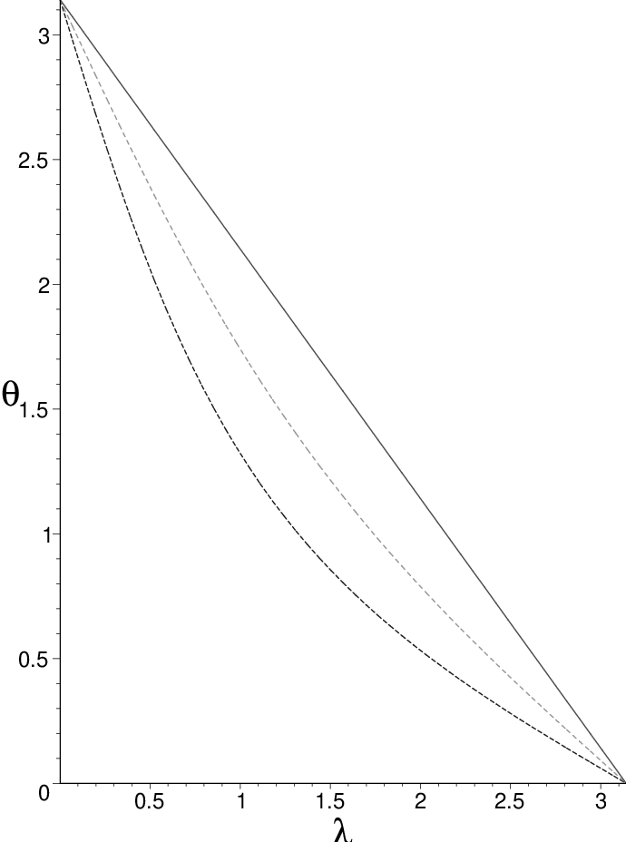
makes it clear that there are precisely $M$ nontrivial eigenoperator solutions for any value of $c_{J}$. The apparently ($M+1$)th solution $\lambda=\pi$ is spurious. This is because, in this case, the left and right moving $k$ dependence is identical ($e^{ik\pi}=e^{-ik\pi}$) and the limit $\lambda\to\pi$ implies $C^{\prime}\to-C$ and $D^{\prime}\to-D$. Thus the corresponding eigenoperators, proportional to $C+C^{\prime}$ and $D+D^{\prime}$, vanish. For comparison, we show $\theta(\lambda)$ and the solution of the eigenvalue equation for several noncritical values $J<\xi$ in Fig. 3.

Applying an eigenoperator to an eigenstate of ${\cal T}$ with eigenvalue $T_{0}$ produces another eigenstate of ${\cal T}$ with eigenvalue $tT_{0}$. We can say that the eigenoperator has increased the energy of the state by an amount $\omega_{\pm}=-\ln t_{\pm}=\pm\omega$. We show $\omega(\lambda)$ for a critical case $\xi=J$ in Fig. 4 and for a noncritical case in Fig. 5.

The fact that the eigenvalue spectrum is non-degenerate guarantees that the set of eigenoperators is complete.

The critical case allows a nontrivial continuum limit $M\to\infty$: In that limit there are finite energy excitations which have $\lambda=O(1/M)$. In this limit the eigenvalue condition simplifies even further to

$\displaystyle e^{i(2M+c_{J})\lambda}=-1+O(\lambda^{2}),\qquad{\rm for}~M\to\infty,~\lambda M~{\rm fixed}\;.$

(36)

or $\lambda=(n+1/2)\pi/M$, which is the mode quantization of the Neveu-Schwarz worldsheet field.

In this section we express the eigenoperators in terms of the $S$’s. We write the eigenoperator as

$\displaystyle A=\sum_{k=1}^{M}(S_{k}^{z}U_{k}+S_{k}^{y}V_{k}),\qquad{\cal T}A{\cal T}^{-1}=tA\;.$

(37)

Then we easily derive the recursion relations satisfied by the $U,V$:

	$\displaystyle tU_{k}$	$\displaystyle=$	$\displaystyle c_{J}c_{\xi}U_{k}-s_{J}s_{\xi}U_{k+1}+ic_{J}s_{\xi}V_{k}-is_{J}c_{\xi}V_{k-1},\qquad k=2,\ldots,M-1$		(38)
	$\displaystyle tV_{k}$	$\displaystyle=$	$\displaystyle c_{J}c_{\xi}V_{k}-s_{J}s_{\xi}V_{k-1}-ic_{J}s_{\xi}U_{k}+is_{J}c_{\xi}U_{k+1},\qquad k=2,\ldots,M-1$		(39)
	$\displaystyle tU_{1}$	$\displaystyle=$	$\displaystyle c_{\xi}U_{1}-s_{j}s_{\xi}U_{2}+ic_{J}s_{\xi}V_{1}$		(40)
	$\displaystyle tV_{1}$	$\displaystyle=$	$\displaystyle-is_{\xi}U_{1}+c_{J}c_{\xi}V_{1}+is_{J}c_{\xi}U_{2}$		(41)
	$\displaystyle tU_{M}$	$\displaystyle=$	$\displaystyle c_{J}c_{\xi}U_{M}-is_{J}c_{\xi}V_{M-1}+is_{\xi}V_{M}$		(42)
	$\displaystyle tV_{M}$	$\displaystyle=$	$\displaystyle c_{\xi}V_{M}-ic_{J}s_{\xi}U_{M}-s_{J}s_{\xi}V_{M-1}\;.$		(43)

The last four special cases will be included in the first two generic equations if we put

$\displaystyle is_{J}V_{0}=(c_{J}-1)U_{1},\qquad-is_{J}U_{M+1}=(c_{J}-1)V_{M}\;,$

(44)

which specify the boundary conditions. As before, these relations can be solved with the plane wave ansatz:

$\displaystyle U_{k}=Ce^{ik\lambda}+C^{\prime}e^{-ik\lambda},\qquad V_{k}=De^{ik\lambda}+D^{\prime}e^{-ik\lambda}\;,$

(45)

leading to

	$\displaystyle{D\over C}$	$\displaystyle=$	$\displaystyle-i{t-c_{J}c_{\xi}+e^{i\lambda}s_{J}s_{\xi}\over c_{J}s_{\xi}-e^{-i\lambda}s_{J}c_{\xi}}$		(46)
	$\displaystyle{D^{\prime}\over C^{\prime}}$	$\displaystyle=$	$\displaystyle-{D^{*}\over C^{*}}\;,$		(47)

together with the consistency condition

$\displaystyle t^{2}-2t(c_{J}c_{\xi}-s_{J}s_{\xi}\cos\lambda)+1=0\;,$

(48)

which is identical to (15). Note that $D/C$ is similar to $B/A$, but not identical to it. This is because the matrix we are diagonalizing is not hermitian. Of course, since the characteristic equation is the same for both eigenvalue problems, the eigenvalue spectrum will be identical. The boundary conditions read

	$\displaystyle is_{J}(D+D^{\prime})$	$\displaystyle=$	$\displaystyle(c_{J}-1)(Ce^{i\lambda}+C^{\prime}e^{-i\lambda})$		(49)
	$\displaystyle-is_{J}(Ce^{i(M+1)\lambda}+C^{\prime}e^{-i(M+1)\lambda})$	$\displaystyle=$	$\displaystyle(c_{J}-1)(De^{iM\lambda}+D^{\prime}e^{-iM\lambda})\;,$		(50)

which lead to

$\displaystyle{C^{\prime}\over C}={is_{J}(D/C)-(c_{J}-1)e^{i\lambda}\over is_{J}(D^{*}/C^{*})+(c_{J}-1)e^{-i\lambda}}\;,$

(51)

and to the consistency condition

	$\displaystyle e^{2iM\lambda}$	$\displaystyle=$	$\displaystyle{(is_{J}(D/C)-(c_{J}-1)e^{i\lambda})(-is_{J}e^{-i\lambda}+(c_{J}-1)(D^{*}/C^{*}))\over(is_{J}(D^{*}/C^{*})+(c_{J}-1)e^{-i\lambda})((c_{J}-1)(D/C)+is_{J}e^{i\lambda})}$		(52)
		$\displaystyle=$	$\displaystyle{is_{J}(1+|D/C|^{2})+2{\rm Re}(e^{-i\lambda}D/C)+2ic_{J}{\rm Im}(e^{-i\lambda}D/C)\over is_{J}(1+|D/C|^{2})-2{\rm Re}(e^{-i\lambda}D/C)+2ic_{J}{\rm Im}(e^{-i\lambda}D/C)}$		(53)
		$\displaystyle=$	$\displaystyle{is_{J}+{\rm Re}(e^{-i\lambda}D/C)+ic_{J}{\rm Im}(e^{-i\lambda}D/C)\over is_{J}-{\rm Re}(e^{-i\lambda}D/C)+ic_{J}{\rm Im}(e^{-i\lambda}D/C)}\;.$		(54)

The last line follows because one can show that $C/D$ is a pure phase. Plugging the solution for $t$ in the equation for $D/C$ and a little manipulation shows that

	$\displaystyle e^{-i\lambda}{D\over C}$	$\displaystyle=$	$\displaystyle-i{\pm\sqrt{(c_{J}c_{\xi}-s_{J}s_{\xi}\cos\lambda)^{2}-1}+is_{J}s_{\xi}\sin\lambda\over c_{J}s_{\xi}\cos\lambda-s_{J}c_{\xi}+ic_{J}s_{\xi}\sin\lambda}$		(55)
		$\displaystyle\to$	$\displaystyle-{\pm\sqrt{1+s^{2}_{j}\sin^{2}(\lambda/2)}+is_{J}\cos(\lambda/2)\over c_{J}(i\sin(\lambda/2)+\cos(\lambda/2))}\;,$		(56)

where the last line shows the simplifying critical limit $\xi\to J$. In this limit we also evaluate

	$\displaystyle{\rm Re}\left[e^{-i\lambda}{D\over C}\right]$	$\displaystyle=$	$\displaystyle-{1\over c_{J}}\cos{\lambda\over 2}\left(\pm\sqrt{1+s^{2}_{J}\sin^{2}{\lambda\over 2}}+s_{J}\sin{\lambda\over 2}\right)$		(57)
	$\displaystyle s_{J}+c_{J}{\rm Im}\left[e^{-i\lambda}{D\over C}\right]$	$\displaystyle=$	$\displaystyle\sin{\lambda\over 2}\left(\pm\sqrt{1+s^{2}_{J}\sin^{2}{\lambda\over 2}}+s_{J}\sin{\lambda\over 2}\right)\;.$		(58)

Then the quantization condition on $\lambda$ simplifies dramatically to

$\displaystyle e^{2iM\lambda}$

$\displaystyle=$

$\displaystyle-{\cos{(\lambda/2)}-ic_{J}\sin{(\lambda/2)}\over\cos{(\lambda/2)}+ic_{J}\sin{(\lambda/2)}}\ =\ -{1-ic_{J}\tan{(\lambda/2)}\over 1+ic_{J}\tan{(\lambda/2)}}\;,$

(59)

which is, of course, identical to (35).

In the Neveu-Schwarz model the G-parity is a crucial symmetry concept. The fermionic raising and lowering operators $b_{r}=b^{\dagger}_{-r}$ are moded with respect to $R=\sum_{r>0}rb_{-r}br$ by half odd integers. G-parity is defined by $Gb_{r}G=-b_{r}$, and $G^{2}=1$. Defining fermion number as $N_{F}=\sum_{r>0}b_{-r}b_{r}$, $G$ is essentially $(-)^{N_{F}}$. Because of the circumstance that the $b$’s carry half odd mode number, we could also write $(-)^{N_{F}}=(-)^{2R}$ which leads to technical simplifications in analyzing the model. The importance of the symmetry is that, since the interactions conserve G-parity, it is consistent to restrict the open string spectrum to be even under G-parity. Since the lowest odd G-parity state is a tachyon, and the lowest even G-parity state is a massless vector, the restriction to even G-parity removes the tachyon, leaving a massless sector that can describe a gauge boson. With this convention for even and odd, $G=-(-)^{N_{F}}=-(-)^{2R}$.

There is no lattice analog of ${N_{F}}$ that commutes with the transfer matrix of the Ising model. However, there is a candidate for $(-)^{N_{F}}$, namely $G=\eta\prod_{k}\sigma_{k}^{x}$, with $\eta^{2}=1$. This operator, which anticommutes with $S_{k}^{y,z}$, commutes with the transfer matrix. The Neveu-Schwarz model in $D$ space-times dimensions requires $D-2$ transverse components ${\boldsymbol{H}}$ and therefore $D-2$ Ising systems, describable by $D-2$ sets of Pauli matrices $\sigma^{x,y,z}_{iA}$, $A=1,\ldots,D-2$. Then the total G-parity operator will be $\eta\prod_{kA}\sigma^{x}_{kA}$. It remains to fix the value of $\eta=\pm 1$. According to the conventions of the Neveu-Schwarz model, we would like it to have the value $-1$ on the ground state of the system when it is critical. Since the ground state at general $J$ has only been determined implicitly by rather complicated equations, it would seem a daunting task to evaluate the action of $G$ on it. However, because $G$ takes on only the values $\pm 1$, its value cannot change under the variation of a continuous parameter. Thus we can exploit simplifications in the state that occur when $J\to 0$ at fixed $\xi$ and $M$.

As we can see from Fig. 3, the eigenvalue problem varies continuously as $J$ decreases continuously from the $J=\xi$ to $J=0$. In the limit $J\to 0$ the eigenvalue equation smoothly approaches

$\displaystyle e^{2iM\lambda}$

$\displaystyle=$

$\displaystyle e^{-2i\lambda},\quad\Rightarrow\lambda={n\pi\over M+1},\qquad n=1,\cdots,M\;.$

(60)

Furthermore the eigenvalues $t_{\pm}(\lambda)\to e^{\mp\xi}$, independent of lambda, and the eigenoperators approach

$\displaystyle A_{n}^{\pm}\to 2iC\sum_{k=1}^{M}(S_{k}^{z}\pm iS_{k}^{y})\sin{n\pi k\over M+1}\;.$

(61)

The $A_{n}^{-}$ increase the eigenvalue of a state by the factor $e^{\xi}$. Therefore in the limit the ground state of the system must be annihilated by all the $A_{n}^{-}$. Since the mode functions $\sin(n\pi k/(M+1))$ are complete, this limiting state must satisfy

$\displaystyle(S_{k}^{z}-iS_{k}^{y})|G_{0}\rangle=0,\qquad{\rm for~all}~k=1,\cdots,M\;.$

(62)

But $\sigma_{k}^{x}=i\sigma_{k}^{z}\sigma_{k}^{y}=2iS_{k}^{z}S_{k}^{y}$ so it follows that

	$\displaystyle\sigma_{k}^{x}|G_{0}\rangle$	$\displaystyle=$	$\displaystyle 2iS_{k}^{z}(-iS_{k}^{z})|G_{0}\rangle=|G_{0}\rangle,\qquad{\rm for~all}~k$		(63)
	$\displaystyle\prod_{k}\sigma^{x}_{k}|G_{0}\rangle$	$\displaystyle=$	$\displaystyle+|G_{0}\rangle\;.$		(64)

By continuity we conclude that the ground state at all $J<\xi$ will have this same eigenvalue. This conclusion depends on the equations determining the ground state not changing discontinuously at some point. For example if the eigenvalue of an eigenoperator changed from $t>1$ to $t<1$ (from $\omega<0$ to $\omega>0$) as $J$ was varied, it would no longer annihilate the ground state and vice versa. But the character of the eigenvalue solutions doesn’t allow this to happen, as is evident from Fig. 3. In particular note that the curve in Fig. 5 stays well away from $\omega=0$ throughout. We conclude that $\eta=-1$, so the correct G-parity operator to use in describing the Neveu-Schwarz model is $G=-\prod_{kA}\sigma^{x}_{kA}$.

Finally, we work out the meaning of G-parity in the language of the original Ising partition function (1). To do this, focussing on a single Ising system, we consider the product of the appropriate factors of $G$ with the transfer matrix (3):

$\displaystyle\prod_{k}\sigma_{k}^{x}{\cal T}$

$\displaystyle=$

$\displaystyle(e^{J^{\prime}}-e^{-J^{\prime}})^{-M/2}\prod_{k}\left(e^{-J^{\prime}/2}+\sigma_{k}^{x}e^{J^{\prime}/2}\right)\exp\left\{{J\over 2}\sum_{k}\sigma_{k}^{z}\sigma_{k+1}^{z}\right\}\;,$

(65)

compared to

$\displaystyle{\cal T}$

$\displaystyle=$

$\displaystyle(e^{J^{\prime}}-e^{-J^{\prime}})^{-M/2}\prod_{k}\left(e^{J^{\prime}/2}+\sigma_{k}^{x}e^{-J^{\prime}/2}\right)\exp\left\{{J\over 2}\sum_{k}\sigma_{k}^{z}\sigma_{k+1}^{z}\right\}\;.$

(66)

Thus, inserting a $G$ somewhere in the matrix element (2) has the effect on (1) of multiplying $Z$ by an overall factor $(-1)$ and reversing the sign of one of the terms in the sum over $j$, $J^{\prime}\sum_{j}(\sum_{kA}\sigma_{kA}^{j}\sigma_{kA}^{j+1})/2$. Technically this is accomplished by inserting a factor $-e^{-J^{\prime}\sum_{kA}\sigma_{kA}^{l}\sigma_{kA}^{l+1}}$, for a particular time slice $l$, in the summand of (1). To project onto even G-parity states, simply insert the factor $(1-e^{-J^{\prime}\sum_{kA}\sigma_{kA}^{l}\sigma_{kA}^{l+1}})/2$. Or perhaps a better way to say it is to make the replacement

$\displaystyle e^{J^{\prime}\sum_{kA}\sigma_{kA}^{l}\sigma_{kA}^{l+1}/2}\to\sinh\left\{{J^{\prime}\over 2}\sum_{kA}\sigma_{kA}^{l}\sigma_{kA}^{l+1}\right\}$

(67)

on at least one time slice of each open string propagator. This sinh factor is non local and also can be negative. The nonlocality would add to the computational cost of a Monte Carlo simulation. This is because the probabilistic criterion for retaining an update of the spin on a site $k,l$ requires knowledge of all the other sites on the time slice $l$, as well as those on neighboring time slices. However, the one-dimensionality of this nonlocality may help keep the cost manageable. The strict probabilistic interpretation of the summand of $Z$, which is the theoretical basis for Monte Carlo simulations, is marred by the fact that the sinh is negative for some spin configurations. However the spin configurations where the argument of the sinh is negative are strongly suppressed by the exponential factors on the many other time slices. One can then hope that those configurations will cause a minimal degradation of the convergence of the simulation.

References

- [1] A. Neveu and J. Scherk, Nucl. Phys. B 36 (1972) 155.
- [2] J. Dai, R. G. Leigh and J. Polchinski, Mod. Phys. Lett. A 4 (1989) 2073.
- [3] J. Maldacena, Adv. Theor. Math. Phys. 2, 231 (1998), hep-th/9711200.
- [4] G. ’t Hooft, Nucl. Phys. B72 (1974) 461.
- [5] K. Bardakci and C. B. Thorn, Nucl. Phys. B 626 (2002) 287 [arXiv:hep-th/0110301]; C. B. Thorn, Nucl. Phys. B 637 (2002) 272 [Erratum-ibid. B 648 (2003) 457] [arXiv:hep-th/0203167]; S. Gudmundsson, C. B. Thorn and T. A. Tran, Nucl. Phys. B 649 (2003) 3 [arXiv:hep-th/0209102].
- [6] D. Chakrabarti, J. Qiu and C. B. Thorn, Phys. Rev. D 72 (2005) 065022 [arXiv:hep-th/0507280]; D. Chakrabarti, J. Qiu and C. B. Thorn, Phys. Rev. D 74 (2006) 045018 [Erratum-ibid. D 76 (2007) 089901] [arXiv:hep-th/0602026].
- [7] R. Giles and C. B. Thorn, Phys. Rev. D 16 (1977) 366.
- [8] S. Mandelstam, Nucl. Phys. B 64 (1973) 205;
- [9] P. Goddard, J. Goldstone, C. Rebbi and C. B. Thorn, Nucl. Phys. B 56 (1973) 109.
- [10] C. B. Thorn, Phys. Rev. D 80 (2009) 086010 [arXiv:0906.3742 [hep-th]].
- [11] C. B. Thorn, Phys. Rev. D 78 (2008) 106008 [arXiv:0809.1085 [hep-th]].
- [12] A. Neveu and J. H. Schwarz, Nucl. Phys. B 31 (1971) 86.
- [13] A. Neveu, J. H. Schwarz and C. B. Thorn, Phys. Lett. B 35 (1971) 529.
- [14] S. Mandelstam, private communication, 1971.
- [15] F. Gliozzi, J. Scherk and D. I. Olive, Phys. Lett. B 65, 282 (1976); Nucl. Phys. B 122 (1977) 253.
- [16] C. B. Thorn, Phys. Rev. D 78 (2008) 085022 [arXiv:0808.0458 [hep-th]].
- [17] P. Goddard and C. B. Thorn, Phys. Lett. B 40 (1972) 235.
- [18] P. Goddard, C. Rebbi and C. B. Thorn, Nuovo Cim. A 12 (1972) 425.
- [19] S. Mandelstam, Nucl. Phys. B 69 (1974) 77.
- [20] P. Orland, Nucl. Phys. B 278 (1986) 790.
- [21] M. B. Green and N. Seiberg, Nucl. Phys. B 299 (1988) 559.
- [22] P. Goddard, Nuovo Cim. A 4 (1971) 349; A. Neveu and J. Scherk, Nucl. Phys. B 36 (1972) 317.