Scattering amplitudes on the Coulomb branch of super Yang-Mills Thanks: HU-EP-10/22. Talk given at Integrability in Scattering Amplitudes, IAS, April 2010, Loops and Legs in Quantum Field Theory, DESY, April 2010 and Amplitudes 2010, QMUL, May 2010.
Abstract
We discuss planar scattering amplitudes on the Coulomb branch of super Yang-Mills. The vacuum expectation values on the Coulomb branch can be used to regulate infrared divergences. We argue that this has a number of conceptual as well as practical advantages over dimensional regularisation.
1 INTRODUCTION
Scattering amplitudes in super Yang-Mills (SYM) have many surprising properties, especially in the planar limit. Being a massless gauge theory, soft and collinear infrared divergences appear that have to be regulated. After a suitable removal of the universal divergent part one can define a finite part. The latter was found to be surprisingly simple, initially perturbatively [1, 2] and later, via the conjectured AdS/CFT correspondence, at strong coupling [3]. Its form (and that of the five-point amplitude) is believed to be known to all orders in the coupling constant [4] (for reviews see [5, 6]).
Given these impressive developments, one may hope that all-order results can also be derived for amplitudes with six and more external particles, at least in the planar limit. Having this motivation in mind, it makes sense to try to use similar methods at weak and strong coupling. An apparent dissimilarity so far is that at weak coupling, the use of dimensional regularisation is predominant, while at strong coupling a different regulator seems to be more natural, where one considers open strings attached to -branes at a non-zero separation [3, 7, 8, 9].
In the dual field theory, this corresponds to going to the Coulomb branch, and was considered in [10, 11]. We take SYM with gauge group and break it to by means of a Higgs mechanism. This gives rise to massive particles in the broken part of the gauge group, while the particles in the unbroken and parts remain massless. If we scatter particles with labels in the part of the gauge group we can select diagrams where the particles in the loop(s) are in the part by taking . In this way, we arrive at the following situation: The scattered particles are massless, and couple via particles of mass that travel along the perimeter of a given diagram, making the integrals infrared finite.
We will now discuss various properties of the massive amplitudes by means of a one-loop example. We then show how the mass regulator can be used to rederive results obtained previously in dimensional regularisation [2, 12, 13] in a simpler way [14, 15]. We also show that the mass-regulated integrals behave nicely in the Regge limit, and identify a class of integrals giving the correct leading log and next-to leading log contributions to all orders in the coupling constant.
2 ONE-LOOP EXAMPLE
Let us illustrate some features of the massive amplitudes by means of a one-loop example. We denote the (colour-ordered) four-point amplitude, normalised by the tree-level contribution, by . Its expansion in the ‘t Hooft coupling reads . The one-loop contribution is given by a scalar box integral [11], with massless external legs and a uniform mass in the loop.
It is noteworthy that its exact expression in involves logarithms and dilogarithms only. Let us compare this to dimensional regularisation, where the result is a hypergeometric function which depends on , with . When expanding the latter in , one obtains higher transcendental functions, see e.g. equation (B.2) in [2].
Coming back to the Coulomb branch, in practice we will not need in its full generality. There are various interesting limits that one can consider, as we discuss presently.
2.1 Regge limit
We use the usual notation and for the Mandelstam invariants. In the Regge limit , we obtain
| (1) |
where is the Regge trajectory. As we will see, this limit organises integrals contributing to the amplitude in a systematic way. We will also give a simple way of seeing that a single logarithm in appears per loop order.
2.2 Low energy limit
The limit was discussed in [16].
2.3 Small mass limit
Here we take , thereby approaching the massless theory, with the infrared (IR) divergences regulated by . In our one-loop example, we obtain
| (2) | |||||
where we have written the result in a way as to make the origin of the terms manifest. As , we obtain double logarithms per loop order as a result of soft and collinear divergences. These logarithms are the analogs of in dimensional regularisation, where one has
| (3) | |||||
The IR divergences appearing in (2) and (3), which take the form of and , respectively, are well understood. We will be interested in the finite part of (the logarithm of) , which is scheme-independent up to an additive constant.
2.4 Geometrical interpretation
3 HIGHER LOOP ORDERS AND
EXPONENTIATION
Let us now review the structure of higher-loop corrections to scattering amplitudes. In a generic gauge theory one can write the planar amplitude in the following factorised form (see [2] and references therein)
| (4) |
where the r.h.s. is a sum of IR divergent terms and a finite term . If the function is zero, as in our case, the explicit form of is particularly simple. In dimensional regularisation,
| (5) |
Here are the expansion coefficients of the universal cusp anomalous dimension [21], and those of the scheme-dependent collinear anomalous dimension.
The structure of the infrared singular terms when using the mass regulator is [22, 23]
| (6) |
where is the analog of . The infrared terms being universal, we are interested in the finite part (which is equal in both schemes up to a coupling-dependent constant). Surprisingly, the latter also turns out to be very simple [1, 2, 3, 4],
| (7) |
Note that when computing perturbatively in dimensional regularisation, e.g. to two-loop order, equation (4) implies that one needs to know
| (8) |
up to terms of . However, terms in lead to an interference of the type , and therefore the and terms in need to be computed too. Likewise, at each new loop order, all lower-loop results need to be extended by two additional orders in .
Let us now consider equation (8) in mass regularisation [11, 14]. There, we can drop terms that vanish as the regulator goes to zero. This is because we have . This trivial observation has very important practical consequences. In particular, for a calculation at arbitrary loop order, the only information needed about is already given in equation (2).
4 EXTENDED DUAL CONFORMAL SYMMETRY
There is a lot of evidence by now that planar scattering amplitudes in SYM possess a dual (super)conformal symmetry [24, 25]. The symmetry acts in a dual space
| (9) |
where the cyclicity condition , with being the number of scattered particles, is tacitly implied. It can be seen that the loop integrand of e.g. the one-loop box integral has a symmetry under inversions in the dual space, or equivalently, under special conformal transformations,
| (10) |
This symmetry is broken in dimensional regularisation, which is why integrals whose integrand naively has the symmetry were dubbed “pseudo-conformal”. The breaking is believed to be under control on the level of the amplitudes, which are conjectured to satisfy anomalous Ward identities [25] initially derived for certain Wilson loops [4].
We will now argue that the symmetry can be repaired at the level of the loop integrals by refining the Higgs setup discussed above [11]. Let us further break the gauge symmetry from to . In this way, we introduce several particle masses. This changes the on-shell conditions of the scattered particles from to and gives different masses to propagators in the loop,
| (11) |
where . The integral is finite, and moreover it has a symmetry, provided that we act on the masses as well as the dual coordinates,
| (12) |
where
| (13) |
We call extended dual conformal transformations.
This has a natural interpretation in string theory. There, the dual conformal symmetry is viewed as the isometry group of a (T-dual) AdS5 space [3, 9], with being its Poincaré coordinates. Usually, when discussing symmetries in the boundary field theory, one sets the radial coordinate . Here, we simply use a different realisation of the SO(2,4) symmetry with , which leads to the generator (13) (see also [26] for a similar discussion of conformal symmetry).
A comment is that from a conventional viewpoint one might be reluctant to call (12) a symmetry since the transformations relate scattering amplitudes with particles having different masses. However, from the AdS perspective the are regarded as coordinates, just as the dual coordinates . Whichever interpretation one prefers, the upshot is that the amplitudes satisfy the conjectured differential equation . As we will see presently, this has important implications for the loop-level integral basis. Also, those integrals can depend on the kinematical variables only in a specific way. For example, in the four-point case, they can be functions of the following two conformally invariant variables only [11],
| (14) | |||||
| (15) |
where we recall that and .
5 HIGHER LOOP INTEGRAL BASIS
It has been observed and discussed in many papers [24, 27, 28, 29, 30] that the loop integrals contributing to amplitudes in SYM are of a very restricted set. The concept of “pseudo-conformal” integrals has been a useful one, although a precise definition of which integrals are pseudo-conformal and which ones are not is difficult due to the issue of IR divergences. One improvement in the setup we propose is that there is a clear definition of integrals invariant under extended dual conformal transformations, namely equation (12).
It is natural to speculate that at a given loop order , the amplitude can be written as a linear combination of integrals satisfying (12), with certain coefficients ,
| (16) |
It is obviously very useful to know in advance which integrals can appear in a calculation, as is the case at one-loop order.
In practice it is easy to write down all dual conformal integrals at a given loop order and number of external particles (e.g. using dual graphs). We remark that an implication of the symmetry is that all triangle subgraphs be absent. At one loop, this necessary requirement was shown to hold [31] (see also [10]).
If the dual conformal ansatz is to reproduce the scattering amplitude , it must have the correct infrared structure, which in the equal mass case is dictated by equations (4) and (6). In general this implies relations between the coefficients appearing in (16). As we will see, these IR consistency equations are in some cases sufficient to determine the .
The two-loop four-point amplitude serves as an illustration of the last statement, since only a single integral is allowed by dual conformal symmetry, whose normalisation is fixed by the exponentiation of IR divergences [11].
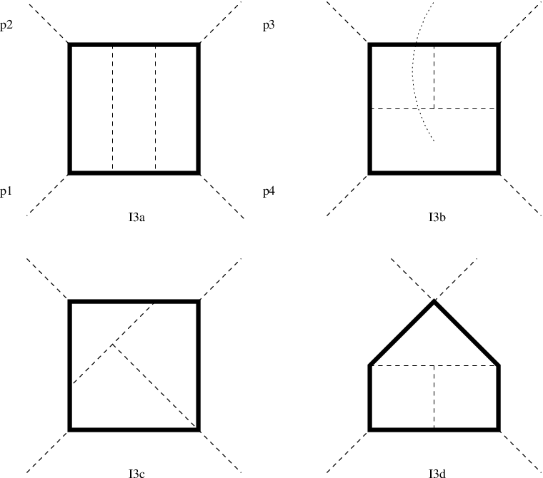
At three loops and four points, there are four dual conformal integrals as shown in Fig. 1. Therefore our ansatz (16) becomes [14]
| (17) | |||||
Let us for the moment set for simplicity. Then the infrared consistency equation, obtained by expanding (4) and (6) to three-loop order and plugging in the known two-loop data, reads
| (18) | |||||
On the other hand, we can explicitly compute the asymptotic expansion of the three-loop integrals. To this end, we write down Mellin-Barnes representations of the integrals, and use the Mathematica packages MB [32] and MBasymptotics [33] to perform the small expansion. We obtain
| (19) | |||||
| (20) | |||||
| (21) |
This obviously determines and , while the coefficients and remain arbitrary. We remark that in dimensional regularisation, one obtains the coefficients , , and [2]. It would be interesting to ascertain the values of the in the mass regulated setup by a direct computation.
We can nevertheless check the consistency of the ansatz (17) with (7). Indeed, if and/or are non-zero, they could be accommodated by a change of the three-loop values of and the three-loop constant in the finite part of . We have checked numerically [14] for various values of that (17) is in agreement with (7).
We remark that while the coefficients of the logarithms in (18) are rather simple, the ones in the results for and are more complicated. Perhaps a better way of performing the calculation exists which avoids the relative complexity of the intermediate results.
In a recent paper, we have extended our computations of the four-point amplitude to the four-loop level [15]. We numerically reproduce the known result for the four-loop value of the cusp anomalous dimension. Perhaps it is a good illustration of the power of the mass regulator that we improve the numerical accuracy of the initial computation [12] by five digits and that of the subsequent computation [13] by two digits.
6 REGGE LIMIT
In the Regge limit one expects the four-point amplitude to have the following form,
| (22) |
Expanding (22) in the coupling constant, at loops the leading and next-to leading logarithm (LL and NLL) will be and , respectively.
We showed in [14, 15] that the LL and NLL terms can be obtained from a simple class of ladder diagrams and ladders with H-shaped insertions, see Fig. 2. Note that this simple pattern is not present in dimensional regularisation.

Dual conformal symmetry allows us to make an interesting observation [14]. Recall that the four-point amplitude is a function of and defined in (14) and (15), and the Regge limit implies . If we set and , we have
| (23) |
and taking , we recover the Regge limit of the original scattering process. However, our new setup corresponds to a “Bhabha-like” scattering process, where heavy particles of approximate mass exchange lighter particles of mass , at fixed and . The absence of collinear divergences in such a process implies that only single logarithms in appear per loop order, in agreement with (22).
ACKNOWLEDGMENTS
We are grateful to the organisers of the conferences where this talk was given for their invitation and to the participants for many interesting discussions. It is a pleasure to thank F. Alday, S. Naculich, J. Plefka, H. Schnitzer, T. Schuster and M. Spradlin for collaboration on the topics presented here.
References
- [1] C. Anastasiou, Z. Bern, L. J. Dixon and D. A. Kosower, Phys. Rev. Lett. 91 (2003) 251602 [arXiv:hep-th/0309040].
- [2] Z. Bern, L. J. Dixon and V. A. Smirnov, Phys. Rev. D 72 (2005) 085001 [arXiv:hep-th/0505205].
- [3] L. F. Alday and J. M. Maldacena, JHEP 0706 (2007) 064 [arXiv:0705.0303 [hep-th]].
- [4] J. M. Drummond, J. Henn, G. P. Korchemsky and E. Sokatchev, Nucl. Phys. B 826 (2010) 337 [arXiv:0712.1223 [hep-th]].
- [5] L. F. Alday and R. Roiban, Phys. Rept. 468 (2008) 153 [arXiv:0807.1889 [hep-th]].
- [6] J. M. Henn, Fortsch. Phys. 57 (2009) 729 [arXiv:0903.0522 [hep-th]].
- [7] H. Kawai and T. Suyama, Nucl. Phys. B 794 (2008) 1 [arXiv:0708.2463 [hep-th]].
- [8] J. McGreevy and A. Sever, JHEP 0808 (2008) 078 [arXiv:0806.0668 [hep-th]].
- [9] N. Berkovits and J. Maldacena, JHEP 0809 (2008) 062 [arXiv:0807.3196 [hep-th]].
- [10] R. M. Schabinger, arXiv:0801.1542 [hep-th].
- [11] L. F. Alday, J. M. Henn, J. Plefka and T. Schuster, JHEP 1001 (2010) 077 [arXiv:0908.0684 [hep-th]].
- [12] Z. Bern, M. Czakon, L. J. Dixon, D. A. Kosower and V. A. Smirnov, Phys. Rev. D 75 (2007) 085010 [arXiv:hep-th/0610248].
- [13] F. Cachazo, M. Spradlin and A. Volovich, Phys. Rev. D 75 (2007) 105011 [arXiv:hep-th/0612309].
- [14] J. M. Henn, S. G. Naculich, H. J. Schnitzer and M. Spradlin, JHEP 1004 (2010) 038 [arXiv:1001.1358 [hep-th]].
- [15] J. M. Henn, S. G. Naculich, H. J. Schnitzer and M. Spradlin, arXiv:1004.5381 [hep-th].
- [16] A. Gorsky and A. Zhiboedov, arXiv:0911.3626 [hep-th].
- [17] L. Mason and D. Skinner, arXiv:1004.3498 [hep-th].
- [18] A. I. Davydychev and R. Delbourgo, J. Math. Phys. 39 (1998) 4299 [arXiv:hep-th/9709216].
- [19] A. Hodges, arXiv:1004.3323 [hep-th].
- [20] N. Arkani-Hamed, F. Cachazo, C. Cheung and J. Kaplan, JHEP 1003 (2010) 020 [arXiv:0907.5418 [hep-th]].
- [21] I. A. Korchemskaya and G. P. Korchemsky, Phys. Lett. B 287 (1992) 169.
- [22] G. P. Korchemsky, Phys. Lett. B 220 (1989) 629.
- [23] A. Mitov and S. Moch, JHEP 0705 (2007) 001 [arXiv:hep-ph/0612149].
- [24] J. M. Drummond, J. Henn, V. A. Smirnov and E. Sokatchev, JHEP 0701 (2007) 064 [arXiv:hep-th/0607160].
- [25] J. M. Drummond, J. Henn, G. P. Korchemsky and E. Sokatchev, Nucl. Phys. B 828 (2010) 317 [arXiv:0807.1095 [hep-th]].
- [26] A. Jevicki, Y. Kazama and T. Yoneya, Phys. Rev. Lett. 81 (1998) 5072 [arXiv:hep-th/9808039].
- [27] J. M. Drummond, G. P. Korchemsky and E. Sokatchev, Nucl. Phys. B 795 (2008) 385 [arXiv:0707.0243 [hep-th]].
- [28] D. Nguyen, M. Spradlin and A. Volovich, Phys. Rev. D 77 (2008) 025018 [arXiv:0709.4665 [hep-th]].
- [29] Z. Bern, J. J. M. Carrasco, H. Johansson and D. A. Kosower, Phys. Rev. D 76 (2007) 125020 [arXiv:0705.1864 [hep-th]].
- [30] Z. Bern, L. J. Dixon, D. A. Kosower, R. Roiban, M. Spradlin, C. Vergu and A. Volovich, Phys. Rev. D 78 (2008) 045007 [arXiv:0803.1465 [hep-th]].
- [31] R. H. Boels, arXiv:1003.2989 [hep-th].
- [32] M. Czakon, Comput. Phys. Commun. 175 (2006) 559 [arXiv:hep-ph/0511200].
- [33]
M. Czakon,
http://projects.hepforge.org/mbtools/.