Cross-Band Interference Considered Harmful in OFDM Based Distributed Spectrum Sharing
Abstract
In the past few years we have witnessed the paradigm shift from static spectrum allocation to dynamic spectrum access/sharing. Orthogonal Frequency-Division Multiple Access (OFDMA) is a promising mechanism to implement the agile spectrum access. However, in wireless distributed networks where tight synchronization is infeasible, OFDMA faces the problem of cross-band interference. Subcarriers used by different users are no longer orthogonal, and transmissions operating on non-overlapping subcarriers can interfere with each other. In this paper, we explore the cause of cross-band interference and analytically quantify its strength and impact on packet transmissions. Our analysis captures three key practical artifacts: inter-link frequency offset, temporal sampling mismatch and power heterogeneity. To our best knowledge, this work is the first to systematically analyze the cause and impact of cross-band interference. Using insights from our analysis, we then build and compared three mitigating methods to combat cross-band interference. Analytical and simulation results show that placing frequency guardband at link boundaries is the most effective solution in distributed spectrum sharing, while the other two frequency-domain methods are sensitive to either temporal sampling mismatch or inter-link frequency offset. We find that the proper guardband size depends heavily on power heterogeneity. Consequently, protocol designs for dynamic spectrum access should carefully take into account the cross-band interference when configuring spectrum usage.
Keywords:
OFDMA , Cross-band Interference , Distributed Network , Dynamic Spectrum Access1 Introduction
In the past few years we have witnessed the paradigm shift from static spectrum allocation to dynamic spectrum access/sharing [1, 2]. In this new model, wireless devices no longer operate on statically assigned spectrum, but acquire spectrum on-demand and share with peers in their local neighborhood. Now wireless devices can obtain spectrum they really need, while improving spectrum utilization through multiplexing.
To realize dynamic spectrum access, one must enable wireless radios to configure and adapt their frequency usage on-the-fly. The widely-known radio solution is orthogonal frequency division multiple access (OFDMA) [3, 4, 5, 6], where a large spectrum band is divided into many frequency subcarriers and an OFDMA radio can access spectrum dynamically by communicating on any combination of the subcarriers. Spectrum multiplexing is achieved by assigning non-overlapping sets of the subcarriers to different users. Using the IDFT/DFT (inverse discrete Fourier transform/discrete Fourier transform) based modulation, all the subcarriers appear orthogonal to each other. Due to its good flexibility and simplicity in implementation, OFDMA has already been applied in IEEE 802.16e (WIMAX) [7] standard.
OFDMA radios, however, are highly sensitive to errors in time and frequency synchronization. Imperfect synchronization destroys the orthogonality among subcarriers and results in inter-carrier interference (ICI) [8]. In centralized networks like WiMAX, an effective way for mitigating ICI is to improve the time and frequency synchronization precision [9, 10, 11]. And in MIMO-OFDM system, in addition to ICI, cross-antenna interference [12, 13] is also one of the main concerns. While in distributed networks, the concurrent asynchronous transmissions produce harmful interference to each other. Moreover, the out-of-band emissions (OOB) and the asynchronism induced cross-band interference cannot be simply filtered out as it leaks into the useful signal’s spectrum [13, 14]. The problem of OOB mitigation in OFDM systems has been studied, and time/frequency domain mitigating methods have been proposed. Windowing based methods [15, 16] mitigate the signal’s power leakage in time-domain, while frequency domain methods deal with this problem by either inserting frequency guardband [15] or performing cancellation coding [17, 18, 19] or using multiple choice sequences approach (MCS) [20]. However, most existing works analyze the unwanted power leakage from the view of the transmitter or its corresponding receiver, which may be different from the view of other receivers as links are asynchronous.
In this paper, we consider the distributed spectrum sharing in wireless systems where no central control is present and tight time synchronization becomes infeasible. In this case, we show that cross-band interference can be highly harmful and lead to large performance degradation. To better understand this special type of interference, we develop a systematic framework to evaluate its impact on asynchronous OFDMA transmissions from the receiver’s point of view. We seek to understand in detail the origin and characteristics of the cross-band interference, examine its impact on packet detection and transmission, and identify effective solutions to suppress the interference. This work builds on our prior work [14] that preliminarily examines the strength of cross-band interference, but makes more comprehensive analysis on the cross-band interference and extends to examine how cross-band interference affects preamble detection and packet reception in the presence of channel fading.
We use a two-step process to analyze cross-band interference. We start from deriving the amount of interference a subcarrier can produce on neighboring subcarriers occupied by other transmissions. Three key practical artifacts are captured: inter-link frequency offset, temporal sampling mismatch and power heterogeneity. Our analysis produces the statistically average interference strength experienced by any frequency subcarrier. Next, we analyze the impact of cross-band interference on packet level performance by examining how cross-band interference affects packet synchronization.
Built on the theoretical analysis, we further propose the cross-symbol cancellation (CSC), a new frequency-domain interference cancellation approach, to address the interference in the presence of large temporal mismatch. We then examine and compare three mechanisms for tackling cross-band interference: frequency guardband (FGB), inter-symbol cancellation (ISC) and CSC. By adding frequency redundancy or overhead to each transmission, these solutions seek to reduce the interference at its source or insert robustness at each receiver against the interference. We examine how these mechanisms perform in distributed networks in the presence of temporal mismatch and inter-link frequency offset. We then evaluate their effectiveness and confirm our conclusions using simulations.
Our work makes two key contributions:
- 1.
We build an analytical model to characterize the impact of cross-band interference on OFDMA transmissions. Our work is the first to analytically evaluate its impact on asynchronous OFDMA transmissions, taking into account the packet synchronization and data reception. Our analytical results closely match the experimental results.
- 2.
We propose a new approach–CSC to tackle cross-band interference. Using both theoretical analysis and simulation experiments, we compare three mitigating methods and show that ISC is ineffective due to temporal mismatch, and CSC is sensitive to frequency offset. Overall, inserting FGB between transmissions is the most efficient solution in distributed spectrum access.
The rest of the paper is organized as follows. In Section 2 we briefly introduce the preliminaries of OFDMA and asynchronous OFDMA. We then in Section 3 characterize the strength of cross-band interference and in Section 4 study its impact on OFDMA operations especially packet synchronization. We propose and analyze three approaches to tackle the interference in Section 5. Simulation results are presented in Section 6 and conclusions are drawn in Section 7 finally.
2 Preliminaries
As background, we briefly discuss the basic operation of OFDMA and the problems it faces when transmissions are asynchronous.
2.1 OFDMA
In OFDMA, each transmitter uses OFDM to transmit signals over their selected subcarriers. The transmitter maps the modulated bit stream into the selected subcarriers, and applies IDFT to convert the bit stream into time-domain OFDM symbols. In this way, it only “pours” power over the selected subcarriers. To decode the OFDM signal, the receiver extracts and adjusts the time-domain symbols through synchronization, and applies DFT to reconstruct the bit stream from the intended subcarriers.
Mathematically, the IDFT and DFT operations can be expressed as:
| (1) |
where is the number of IDFT/DFT points which is often set as the power of so that fast Fourier transform (FFT) and inverse FFT (IFFT) can be used to achieve efficiency. denotes the frequency-domain data on the th subcarrier, is the th sampling point of time-domain OFDM symbol, and is the set of occupied subcarriers. Different links possess non-overlapping s, so multiple transmissions can take place simultaneously in time and be distinguished in frequency.
One important requirement in OFDMA is to maintain the subcarrier orthogonality so that simultaneous transmissions from different subcarriers will not interfere with each other. When transmissions from coexisting links are perfectly synchronized in time and frequency, the DFT operations at their receivers will remove unwanted signals and maintain subcarrier orthogonality.

2.2 Distributed OFDMA
In distributed OFDMA, due to the inherent asynchronism, subcarrier orthogonality across links is destroyed and harmful cross-band interference is created. Figure 1 shows a distributed OFDMA network with two independent links–link 1 and link 2, each occupying a non-overlapping set of subcarriers. The frequency-domain and time-domain snapshots of the two transmissions viewed at link 2’s receiver are shown on the bottom. In this paper, we characterize the distributed OFDMA and the cross-band interference by taking into account the following three artifacts:
- 1.
Inter-link Frequency offset is the central frequency discrepancy between the two links’ transmitters. It keeps stable during a short period if the environmental parameters (such as temperature, humidity) do not change rapidly. We assume subcarrier in this paper.
- 2.
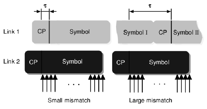
Temporal mismatch refers to the difference between the two links’ symbol arrival time viewed at the receiver, as shown in Figure 1 (right bottom). We assume that is evenly distributed in , where and denote the symbol length (excluding the cyclic prefix) and the cyclic prefix length, respectively.
- 3.
Power Heterogeneity refers to the difference in average power per subcarrier of different transmissions observed at the receiver. The problem of power heterogeneity can be alleviated using power control in cellular network [21], but remains in distributed network as users are not coordinated. is defined as the power ratio of link 1 to link 2.
3 Characterizing Cross-Band Interference
In this section, we examine the cross-band interference in asynchronous OFDMA systems. Using the example in Figure 1, we treat link 1 as the interferer and examine its interference at link 2’s receiver in the presence of the temporal mismatch and inter-link frequency offset. We use the rectangular pulse shaping for OFDM symbols, and assume multipath fading channels of -factor Rician distribution for both links, where the -factor is defined as the ratio of signal power in line-of-sight component over the scattered power. Our study of two-link network can easily apply to the scenario of multiple links.
As shown in Figure 2, we divide our analysis into two cases based on the degree of temporal mismatch: small mismatch when or large mismatch when . To simplify our analysis, we assume the users in this network are homogeneous with the same OFDM parameters. We will examine the impact of user heterogeneity in our future work.
3.1 Case A: Small Temporal Mismatch
From Figure 2, when , each desired OFDM symbol of link 2 will face interference from only one symbol of its interferer. Let represent the frequency-domain data sent by link 1 on subcarrier . At link 2’s receiver, it will experience a phase rotation in the frequency domain due to the temporal mismatch :
| (2) |
where is the total number of subcarriers.
To determine the cross-band interference from link 1 to link 2, we compute the power spectrum of together with the channel response at any continuous frequency . This allows us to determine the interference in the presence of inter-link frequency offset , where link 1’s transmissions at subcarrier # arrive at link 2’s subcarrier #. For example, refers to the frequency location of subcarrier #, and refers to the middle of subcarriers # and #.
Let represent the set of subcarriers occupied by the interferer link 1. We perform discrete-time Fourier transform (DTFT) to derive (), link 1’s power spectrum seen by link 2 at any continuous :
| (3) |
where is the frequency-domain channel response between link 1 and 2, is the interferer’s spectrum represented as:
| (4) |
3.2 Case B: Large Temporal Mismatch
When , each desired OFDM symbol of link 2 will face interference from two truncated symbols of link 1 (see Figure 2). Without loss of generality, we assume it overlaps with symbol I in sampling points and symbol II in points, where is determined by the temporal mismatch (, where refers to rounding up the argument to the nearest integer). Let and represent the frequency-domain constellation points on the th subcarrier from Symbol I and Symbol II respectively. Due to the temporal mismatch, each signal goes through a phase rotation and a truncation based on the non-mismatch symbol where : first, each symbol shifts its sampling location by to the right, which corresponds to ’s phase rotation by , and then Symbol I removes the tail points and Symbol II removes the front points.
The interfering signal’s power spectrum becomes:
| (5) |
where and are the DTFT outputs of the two OFDM symbols respectively:
| (6) |
The derivation of Equation (6) can be found in Appendix A. Because and are randomly chosen from the constellation map and independent of each other, the power spectrum becomes randomly distributed across and is no longer zero at integer locations.
From the above analysis, we see that the cross-band interference at any specific depends heavily on the channel property , temporal mismatch level and the configuration of signal constellation . In the following, we perform statistical analysis to derive the average interference strength.


3.3 Statistical Analysis
To characterize the cross-band interference, we make a statistical analysis to achieve the average cross-band interference strength. Our analysis makes the following assumptions. , and are independent and identically distributed (i.i.d) with constant average power for all , and the average channel gain is unified, i.e., .
Time-Frequency Domain View. We first derive the average interference strength at any frequency location and temporal mismatch pair by averaging over and .
For Case A, with respect to Equation (3), by averaging over the statistical distribution of and , we get the average cross-band interference strength:
| (7) | ||||
We observe that the average cross-band interference under small temporal mismatch () is independent of . This property has been utilized in centralized OFDMA networks that apply cyclic prefix to reduce the impact of imperfect timing synchronization.
For Case B, by averaging over and (which are independent of each other) as well as in Equation (5), the average interference strength becomes:
| (8) | ||||
Figure 3(a) shows the average interference strength (normalized by ) at any (,) pair. As expected, marks an obvious boundary between Case A and B.
Frequency Domain View. To examine the average cross-band interference over time, we take an average over the temporal mismatch . Note that follows a random uniform distribution in as different transmissions may start at random time.
For Case A, Equation (7) is already independent of , thus we have
| (9) |
For Case B, the average cross-band interference strength at any frequency location is the integral of (in Equation (8)) with respect to :
| (10) | ||||
Figure 3(b) shows the average cross-band interference strength as a function of frequency separation. To draw a comparison between the cases of small mismatch (Case A) and large mismatch (Case B), we average the interference strength across one subcarrier’s span, i.e., averaging over in , and so on. The resultant curves labelled by "step" in Figure 3(b) show that the average cross-band interference strength of Case B is stronger by approximately dB than that of Case A.
By combining the results of Case A and B statistically, we derive the overall average interference strength:
| (11) | ||||
where () and are the event probabilities of Case A and B. Note that is equivalent to the additional overhead due to cyclic prefix. Using this result, we are able to evaluate the expected cross-band interference strength at given frequency locations statistically. We also plot the overall average cross-band interference strength in Figure 3(b).
The overall average cross-band interference strength expressed in Equation (11) is determined by the following parameters: the interference link’s power (), the frequency separation to the interferer’s th subcarrier (), the number of subcarriers occupied by the interference link (), the overhead due to cyclic prefix () and the number of FFT/IFFT points (). It is obvious that the cross-band interference increases linearly with the interference link’s power , and decreases quickly as the frequency separation is enlarged. But the impacts of , and are implicit. Next we seek to understand their impacts through numerical calculations, and the results are shown in Figure 4. We see that the average cross-band interference strength slightly increases as gets larger, and experiences a dB reduction at the integer frequency locations when changes from to , and it is almost insensitive to (as can be approximately cancelled). Therefore, based on the above analysis we conclude that:
- 1.
Asynchronous transmissions create cross-band interference to each other due to temporal mismatch and/or inter-link frequency offset;
- 2.
Among those factors that have impacts on the average cross-band interference strength, the interference link’s power and the frequency distance to the interference are dominating.


4 Impact of Cross-Band Interference
An OFDM packet consists of a synchronization-targeted preamble and a number of data symbols. In this section, we focus on the impact of the cross-band interference on packet detection/synchronization, since it affects data reception in frequency domain directly.
4.1 Packet Detection and Synchronization
In OFDM(A) systems, a receiver performs synchronization by detecting the packet preamble and compensates the intra-link frequency offset [22, 23, 24]. In most existing systems including 802.11a [25] and WiMAX [7], preambles are time-domain repeated symbols. To detect a preamble, the receiver uses a delay-correlation structure to produce a peak when the preamble arrives. The location of the peak marks the beginning of data frame, and the phase information extracted from the preamble can be used to estimate the intra-link fractional frequency offset. The integer frequency offset is usually compensated via another pseudo-random noise (PN) sequence in frequency domain afterwards.
Two types of interference from the concurrent transmissions should be considered with respect to packet synchronization. The first and stronger one is the inter-channel interference caused by coexisting users operating on different frequency bands. This type of interference can be effectively mitigated by adding band-pass filter, since the spectrum pattern is known to the receiver. The second one is the cross-band interference which can not be filtered out because it is the power leaked into the desired signal’s main band. To examine the impact of cross-band interference on synchronization performance, we assume that the inter-channel interference is fully filtered out. As to the evaluation metric, we only examine the intra-link frequency offset error, as the timing synchronization precision can be relaxed by adding long cyclic prefix.
4.2 Impact on Packet Synchronization
We use the standard deviation of the intra-link frequency offset error (normalized to subcarrier spacing) and the induced ICI to characterize the synchronization performance.
We quote the preamble analysis in [22]. At high SNRs without considering the interference, the standard deviation of can be estimated as:
| (12) |
where is the number of subcarriers occupied by the signal link, SNR is the average signal to noise power ratio (SNR) over all used subcarriers. To simplify our analysis, we assume the interference signal is Gaussian distributed and independent of the desired signal and noise, so we make a simple approximation by substituting SNR with SINR–the signal to interference-plus-noise power ratio in Equation (12), i.e.,
| (13) |
We as well assume is high, because it is measured over all used subcarriers rather than at specific subcarriers. Thus the average SINR is much lowered as compared with that on the edge subcarriers near to the interferer. The interference power can be estimated in frequency domain:
| (14) |
where is the forementioned inter-link frequency offset.
We next derive the average signal power of link 2. Let represent the set of subcarriers occupied by link 2. Similarly to the analysis in Section 3, we can compute link 2’s power spectrum by:
| (15) |
where is the frequency-domain channel response of link 2, is the desired signal’s spectrum:
| (16) |
where is the frequency domain signal sent by link 2’s transmitter. Assuming and for all , we can derive the average signal strength of link 2 by taking the average of Equation (15):
| (17) |
The residual frequency synchronization error will lead to additional ICI due to the destroyed subcarrier orthogonality. For a given investigated at link 2’s receiver, it deviates from the right subcarrier index by , where . This will result in useful signal’s power loss and unwanted ICI. In this case, Equation (17) can be decomposed into two components:
| (18) |
where and represent signal power and ICI power respectively. We see that is independent of , and is actually insensitive to as well. The detailed analysis of ICI can be found in [26].
4.3 Comparing ICI with Cross-Band Interference
The received data symbols now experience two types of interference: the cross-band interference and the extra ICI due to . The average carrier to interference power ratio (CIR) determines the performance of data retrieval which is defined as:
| (19) |
where , are defined in Equation (18) and is defined in Equation (11). With Equation (19), we are able to compute the bit error rate at specific subcarriers under various flat fading or non-fading channels using conventional analytical approaches [27, 28]. Difference from the cross-band interference, ICI produces almost the same interference power to all relevant subcarriers, because applies to each subcarrier equivalently. Note that CIR is dependent on the power heterogeneity which denotes the difference between and .
ICI is much weaker than the worst case of the cross-band interference, due to the robustness of the synchronization scheme. We use an example to show this property. Let link 1 (the interference link) and link 2 (the signal link) occupy the subcarriers ## and ## out of 64 subcarriers respectively, without inter-link frequency offset nor power heterogeneity (i.e., , ). Also additive white Gaussian noise is added with dB per subcarrier. The analytical results are derived as follows. The normalized can be estimated through Equation (14): dB. Using this result we are able to calculate that dB and (normalized to subcarrier spacing). Even using the adverse case of substituting for in Equation (18), we still achieves tolerable signal loss and ICI: dB and dB. While the average cross-band interference strength at #1 (strongest) and #8 (weakest) are and respectively. From this example we see that
| (20) |
So at the most concerned subcarriers that experience stronger cross-band interference interference, the synchronization error induced ICI can be ignored.
The negligibility of the impact of synchronization errors simplifies our analysis by assuming perfect synchronization. However, when multiple non-contiguous OFDM (NC-OFDM) spectrum blocks are used by one user [29, 30], the cross-band interference from more neighbors would become stronger. In this case, the impact of the cross-band interference on synchronization may not be negligible, which we will study in our future work.
5 Tackling Cross-Band Interference
In this section, we introduce three mechanisms to mitigate cross-band interference. By adding frequency redundancy, these mechanisms seek to reduce the interference each subcarrier leaks to its neighbors, and/or to insert robustness at each receiver against such interference. The first two mechanisms are from prior works and the last mechanism is our new proposal.
5.1 Frequency Guardband (FGB)
Inserting frequency guardband between transmissions is the most straightforward way to mitigate cross-band interference [15]. As shown in Figure 3, the interference strength decreases with the frequency separation. For example, adding one subcarrier as guardband between link 1 and 2 will reduce the interference power from dB to dB. Such dB difference could significantly improve transmission quality. When a frequency guardband of subcarriers is used between two transmissions, the average cross-band interference strength can be derived from the original analysis (Equation (11)) by shifting by subcarriers (become into ). Because guardband is not used for transmissions, this approach leads to extra overhead.
The choice of guardband size depends heavily on power heterogeneity and the minimal CIR requirement . In table 1, we summarize the needed minimal guardband size (normalized to subcarrier spacing), assuming and 8 subcarriers are used by the interference link. From the results we see that larger guardband is needed as the power heterogeneity gets higher. This observation is helpful in designing spectrum allocation strategies.
| 0dB | 3dB | 6dB | 9dB | |
|---|---|---|---|---|
| 5dB | 0 | 0 | 0.6 | 1.6 |
| 10dB | 0.2 | 1.0 | 2.0 | 4.0 |
| 15dB | 1.8 | 3.7 | 5.9 | 10.0 |
5.2 Intra-Symbol Cancellation (ISC)
Another mechanism is to reduce interference strength by carefully controlling the signal pattern. Prior work has proposed a series of approaches [18, 17] where a transmitter codes several subcarriers within one symbol in such a way that their signal sidelobes cancel each other and hence the aggregated sidelobe becomes much smaller. We call this type of interference mitigation methods intra-symbol cancellation (ISC). For example, if a transmitter codes its subcarrier and such that:
| (21) |
then at any time-synchronized receiver, the cross-band interference from and is expected to cancel each other out. In fact, when , according to Equation (4) the sum power spectrum of the th and th subcarriers is
| (22) | ||||
In this case, the interference power decreases more quickly as compared with the non-mitigation case.
This approach, however, faces two key challenges. First, it leads to extra overhead since two subcarriers now only carry the load of one subcarrier. Second and more importantly, ISC is sensitive to the temporal mismatch. Specifically, in the presence of temporal mismatch, each subcarrier has a phase shift as we have shown in Section 3. The phase shift of (in small mismatch) or , (in large mismatch) depends on and , thus the th and th subcarriers experience different phase shifts and their sidelobes cannot effectively cancel each other. Mathematically deriving the interference strength is complex, so later we use simulation results to verify our intuitional analysis.
5.3 Cross-Symbol Cancellation (CSC)
To address the temporal mismatch, we propose to extend coding across symbols, referred to as the cross-symbol cancellation (CSC). In contrast with ISC, CSC modifies every two consecutive OFDM symbols on the same th subcarrier to compensate for the temporal mismatch. Consider and already defined above, after CSC, they become:
| (23) |
The factor compensates the phase shift so that for both Case A and B, the actual interference signal will have continuous phases, thus it can be seen as one completed OFDM symbol. In doing so, no matter how large the temporal mismatch is, the power spectrum of the th subcarrier can be derived as
| (24) |
In this case, the aggregated signal sidelobe can be minimized at integer frequency locations. Like ISC, CSC must trade off the bandwidth overhead for interference mitigation. For example, coding a small set of subcarriers on the frequency edge is more bandwidth-efficient than coding all the subcarriers together, but is less effective in tackling the interference.
There are two steps to follow in the CSC-based system implementation. 1) At the transmitter, all links perform CSC coding on the edging subcarriers across every two successive OFDM symbols, where is chosen according to the system requirements; 2) At the receiver, data symbols are jointly decoded through every two precoded symbols, at least one of which will experience the interferer’s symbols with continuous phases of the subcarriers. Choosing the less-interfered symbol from the two CSC-coded symbols can be assisted with channel estimation or other approaches, but we omit the details due to page limit.
Using the analytical results in the previous section, we verify that CSC is insensitive to the temporal mismatch. More importantly, the cross-band interference strength when is an integer of the subcarriers with full-bits coding. That is, if the frequency offset is zero, the desired signal is sampled at integer and does not experience any cross-band interference. On the other hand, the performance of CSC is sensitive to the inter-link frequency offset. When the offset is 0.5 subcarrier, CSC suffers from almost the same interference as the original system. Therefore, the proposed CSC is suitable for the frequency synchronized network.
6 Evaluation
In this section, we perform Matlab simulations to verify the accuracy of our analytical models and further compare the effectiveness of the three interference mitigation mechanisms.
6.1 Experiment Setup
By default, we simulate two links (link 1 and 2), each occupying 8 frequency subcarriers out of a total of 64 subcarriers. The links operate asynchronously and start their transmissions randomly. Treating link 1 as the interference link, we measure the impact of cross-band interference on link 2’s transmissions. We use four metrics: the interference strength at each subcarrier, the BER at each subcarrier, the impact on packet synchronization and the overall effective link throughput. Similarly we also examine link 2’s performance with and without any interference mitigation mechanisms.
Table 2 summarizes the default simulation parameters. We choose which is the standard configuration in 802.11 systems. We also consider three practical artifacts: power heterogeneity, channel fading and inter-link frequency offset. To examine the impact of power heterogeneity , we configure the interferer strength to be dB stronger than that of the desired signal at their intended subcarriers, i.e. . We then vary to examine the performance when the interferer is stronger or weaker than the target signal. To examine the impact of channel fading, we consider a Rician fading environment and vary the -factor to control the weight of the line-of-sight and the Rayleigh fading components. When , Rician fading becomes Rayleigh fading, which has only scattered signal components. And when , it can be seen as non-fading. For simplicity, we assume .
| Parameter | Value |
| 64 | |
| 16 | |
| Modulation | QPSK |
| Subcarrier bandwidth | 12.5 Hz |
| Desired signal’s bandwidth | 8 subcarriers |
| Interferer’s bandwidth | 8 subcarriers |
| Packet size | 32 OFDM symbols |
| Guardband size | 0 subcarrier |
| (dB) | (dB) | ||||||
| NonFd | Ryl. | Theo. | NonFd | Ryl. | Theo. | ||
| 1 | -9.1 | 5 | -19.2 | ||||
| 2 | -13.5 | 6 | -20.3 | ||||
| 3 | -16.1 | 7 | -21.3 | ||||
| 4 | -17.8 | 8 | -22.1 | ||||
6.2 Evaluating Cross-band Interference
We start from examining the strength of cross-band interference and its impact in terms of the packet synchronization and BER performance.
Interference Strength Measurement. By generating the link 1’s signal and performing DTFT on the received signal at link 2, we measure the average interference power over 10,000 runs. This measurement allows us to verify the accuracy of our analytical model by comparing it with the experimental results. Two typical channels–non-fading channel and Rayleigh fading fading channel are used in our simulations. In Table 3 we list the average signal strength derived from the simulation and our theoretical analysis, where the two results differ by at most dB. We also examined the maximum difference between the two when link 1 uses different number of subcarriers, i.e. varying , and the results match our analysis too.
Impact on Packet Synchronization. We evaluate the interference’s impact on packet synchronization by measuring the statistics of –the intra-link frequency offset error. Using a multi-band filter generated by windowing method (e.g., Hamming), link 1’s main-band interference is filtered out and only cross-band interference leaks into link 2’s receiver. Assuming the actual intra-link frequency offset is randomly distributed in , we run frequency offset estimation and measure the standard deviation of over 10,000 simulations. Figure 5 shows the measurement results, from which we see that the simulation results have smaller standard deviations than the analytical results in the presence of power heterogeneity. One reason for that is the non-Gaussian distributed cross-band interference has weaker impact than the assumed Gaussian distributed one. Assisted by the analysis in Section 4.3, it is reasonable to neglect the impact of the cross-band interference on packet synchronization when evaluating system performance.
BER Performance Measurement. Next, we assume no intra-link synchronization error and focus on examining the BER caused by the cross-band interference. We consider the power heterogeneity and Rician fading with -factor individually. We vary from dB to dB in Rayleigh fading channel (), and consider four channel fading situations: (non-fading), , , and (Rayleigh fading) under large power heterogeneity when dB. Figure 6 shows the simulation results. We see that the BER at each subcarrier increases gracefully as increases, and increases dramatically as decreases (from non-fading to Rayleigh fading).


6.3 Comparing Interference Mitigating Mechanisms
Next, we examine the effectiveness of various interference mitigation mechanisms, using both interference strength and link throughput measurements.
Interference Strength Measurement. We first compare the three mitigating methods–FGB, ISC and CSC with the original system in terms of interference strength. Figure 7 shows the results when these mitigation methods spend 25% overhead to combat the interference. As expected, ISC has little improvement over the original system due to its sensitivity to the random temporal mismatch; CSC reduces the interference strength dramatically only at integer frequency separations, showing its sensitivity to the inter-link frequency offset; while FGB reduces the interference strength significantly, especially at subcarriers that are close to the interferer.
Link Throughput Measurement. We use link throughput measurements to examine the impact of cross-band interference and the mitigation overhead. We turn both link 1 and 2 on, randomly generate 10,000 OFDM packets, each carrying 32 symbols, and measure link 2’s effective throughput. We assume there is no intra-link synchronization error, but link 1 and 2 have a inter-link frequency offset. We also use AWGN channel with dB additive white Gaussian noise.
Because the link throughput depends on the coding overhead in ISC/CSC and the amount of frequency guardband in FGB, we configure the experiments to perform a fair comparison. Assuming a total of 16 subcarriers, we choose the best coding format for ISC/CSC to maximize link 2’s effective throughput, using the same configuration for link 1 and 2. For FGB, we place null subcarriers between link 1 and 2, and split the rest subcarriers between them. We choose the optimal that maximizes the effective throughput.
Figure 8 shows the throughput results where ranges from dB to dB and is randomly distributed in subcarrier. Both CSC and FGB consistently outperform the other two. When the interferer is dB stronger than the desired signal, FGB and CSC provide roughly 100% throughput improvement. FGB outperforms CSC slightly because CSC cannot nullify the interference when . The difference between FGB and CSC is small because is relatively small in our experiments.
Impact of Inter-link Frequency Offset. To examine the impact of inter-link frequency offset, on compare CSC and FGB when the inter-link frequency offset is uniformly distributed in . Results from Figure 9 show that the link throughput of CSC degrades gracefully with , especially when the desired signal is weaker. This can be explained by Figure 7 where the CSC’s cross-band interference increases with . When subcarrier, the interference becomes similar to the no-mitigation case. On the other hand FGB is almost insensitive to .
7 Conclusions and Future Work
In this paper, we consider the problem of distributed spectrum sharing using OFDMA. We show that artifacts from asynchronous transmissions destroy subcarrier orthogonality, creating cross-band interference among transmissions. We develop an analytical framework to quantify the strength of cross-band interference and evaluate its impacts on preamble detection as well as data reception. We show that the cross-band interference is present and can produce large performance degradations. We then build and compare three methods to mitigate the interference. Experimental and analytical results show that adding frequency guardband is the most efficient solution in the presence of temporal mismatch and frequency offset. While choosing the guardband size depends heavily on the power heterogeneity between spectral adjacent links.
We are considering extending our work in the following directions. First, we are currently studying the impact of user heterogeneity, such as power heterogeneity, symbol length heterogeneity etc., on the cross-band interference. Second, our analysis considers flat fading channel in this paper, which can be extended to frequency selective fading channel. Last, using insights of our analysis, it is worthwhile investigating how to integrate the interference mitigation methods into practical dynamic spectrum access protocols.
Appendix A
In the following derivations, we denote , and as the time-domain sampling points of link 1’s signal seen from link 2’s receiver (see Figure 2). refers to the samples in small mismatch case, and and refer to the samples of Symbol I and Symbol II in large mismatch case, respectively.
A.1 Derivation of in Eq. .
Note that reflects the relative cyclic shift of by compared with link 2’s signal.
A.2 Derivation of and in Eq.
Similarly, refer to the sampled points in the time domain, and refer to the symbols in the frequency domain.
References
- [1] I.F. Akyildiza, W.Y. Leea, M.C. Vuran, and S. Mohantya, “NeXt generation/dynamic spectrum access/cognitive radio wireless networks: A survey,” Computer Networks, vol.50, no.13, pp.2127–2159, 2006.
- [2] S. Haykin, “Cognitive radio: brain-empowered wireless communications,” IEEE Journal on Selected Areas in Communications, vol.23, no.2, pp.201–220, 2005.
- [3] H. Yin and S. Alamouti, “OFDMA: A wireless access broadband technology,” IEEE Sarnoff Symposium, 2003.
- [4] S.H. Ali, K.D. Lee, and V.C. Leung, “Dynamic resource allocation in OFDMA wireless metropolitan area networks,” IEEE Transactions on Wireless Communications, vol.14, no.1, pp.6–13, 2007.
- [5] F.S. Chu and K.C. Chen, “Radio resource allocation in OFDMA cognitive radio systems,” Proc. of PIMRC, 2007.
- [6] L. Yang, L. Cao, H. Zheng, and E. Belding, “Traffic-aware dynamic spectrum access,” Proc. of WICON, 2008.
- [7] IEEE Std 802.16e-2005: IEEE Standard for Local and Metropolitan Area Networks Part 16: Air Interface for Fixed and Mobile Broadband Wireless Access Systems, IEEE Press, 2005.
- [8] T. Pollet, M.V. Blade, and M. Moeneclaey, “BER sensitivity of OFDM systems to carrier frequency offset and Wiener phase noise,” IEEE Transactions on Communications, vol.43, no.234, pp.191–193, 1995.
- [9] H. Nguyen, E. de Carvalho, and R. Prasad, “Joint estimation of the timing and frequency offset for uplink OFDMA,” Wireless Personal Comm., 2008.
- [10] M. Morelli, “Timing and frequency synchronization for the uplink of an OFDMA system,” IEEE Transactions on Communications, vol.52, no.2, pp.296–306, 2004.
- [11] M.O.P.C.C.J. Kuo and M. Morelli, “Joint synchronization and channel estimation in uplink OFDMA systems,” Proc. of ICASSP, 2005.
- [12] W. Zhang, Z. Zhang, and C. Tellambura, “Signal-to-interference-plus-noise ratio analysis for MIMO-OFDM with carrier frequency offset and channel estimation errors,” Proc. of WCNC, 2007.
- [13] T. Tang and R.W. Heath, “A space-time receiver with joint synchronization and interference cancellation in asynchronous MIMO-OFDM systems,” IEEE Transactions on Vehicular Technology, vol.57, no.5, pp.2991–3005, 2008.
- [14] W. Hou, L. Yang, L. Zhang, X. Shan, and H. Zheng, “Understanding cross-band interference in unsynchronized spectrum access,” ACM MobiCom’09 Workshop on Cognitive Radio Networks (CoRoNet), 2009.
- [15] T. Weiss, J. Hillenbrand, A. Krohn, and F.K. Jondral, “Mutual interference in OFDM-based spectrum pooling systems,” Proc. of VTC, 2004.
- [16] H.A. Mahmoud and H. Arslanu, “Sidelobe suppression in OFDM-based spectrum sharing systems using adaptive symbol transition,” IEEE Communication Letters, 2008.
- [17] S. Brandes, I. Cosovic, and M. Schnell, “Reduction of out-of-band radiation in OFDM systems by insertion of cancellation carriers,” IEEE Communication Letters, vol.10, no.6, pp.420–422, 2006.
- [18] K. Panta and J. Armstrong, “Spectral analysis of OFDM signals and its improvement by polynomial cancellation coding,” IEEE Trans. on Consumer Electronics, vol.49, no.4, pp.939–943, 2003.
- [19] T. Matsuura, Y. Iida, C. Han, and T. Hashimoto, “Improved algorithms for cancellation carrier optimization to suppress the OFDM OOB spectrum,” IEEE Communication Letters, vol.13, no.2, pp.112–114, 2009.
- [20] I. Cosovic and T. Mazzoni, “Suppression of sidelobes in OFDM systems by multiple-choice sequences,” European Trans. on Telecom., vol.17, no.6, pp.623–630, 2006.
- [21] J. Jang and K.B. Lee, “Transmit power adaptation for multiuser OFDM systems,” IEEE Journal on Selected Areas in Communications, vol.21, no.2, pp.171–178, 2003.
- [22] T.M. Schmidl and D.C. Cox, “Robust frequency and timing synchronization for OFDM,” IEEE Transactions on Communications, vol.45, no.12, pp.1613–1621, 1997.
- [23] H.K. Song, Y.H. You, J.H. Paik, and Y.S. Cho, “Frequency-offset synchronization and channel estimation for OFDM-based transmission,” IEEE Communication Letters, vol.4, no.3, pp.95–97, 2000.
- [24] E.G. Larsson and J. Li, “Preamble design for multiple-antenna OFDM-based WLANs with null subcarriers,” IEEE Transactions on Signal Processing, vol.8, no.11, pp.285–288, 2001.
- [25] IEEE Std 802.11-2007: Wireless LAN Medium Access Control (MAC) and Physical Layer (PHY) specifications, IEEE Press, 2007.
- [26] Y. Zhao and S.G. Hggman, “Intercarrier interference self-cancellation scheme for OFDM mobile communication systems,” IEEE Transactions on Communications, vol.49, no.7, pp.1185–1191, 2001.
- [27] J. Proakis, Digital Communications, four ed., McGraw-Hill Higher Education, 2000.
- [28] M.K. Simon and M.S. Alouini, Digital Communication over Fading Channels, second ed., John Wiley & Sons, 2005.
- [29] H. Tang, “Some physical layer issues of wide-band cognitive radio systems,” Proc. IEEE Int. Symp. New Frontiers Dynamic Spectr. Access Networks, 2005.
- [30] J.D. Poston and W.D. Horne, “Discontiguous OFDM considerations for dynamic spectrum access in idle TV channels,” Proc. IEEE Int. Symp. New Frontiers Dynamic Spectr. Access Networks, 2005.