Abstract
In these lectures I describe the remarkable ultraviolet behavior of supergravity, which through four loops is no worse than that of super-Yang-Mills theory (a finite theory). I also explain the computational tools that allow multi-loop amplitudes to be evaluated in this theory — the KLT relations and the unitarity method — and sketch how ultraviolet divergences are extracted from the amplitudes.
SLAC–PUB–14091
Ultraviolet Behavior of = 8 Supergravity11 1 Presented at International School of Subnuclear Physics, 47th Course, Erice Sicily, August 29-September 7, 2009.
Lance J. Dixon
SLAC National Accelerator Laboratory
Stanford University
Stanford, CA 94309, USA
1 Introduction
Quantum gravity is nonrenormalizable by power counting, because the coupling, Newton’s constant, , is dimensionful. In contrast, the coupling constants of unbroken gauge theories, such as for QED and for QCD, are dimensionless. At each loop order in perturbation theory, ultraviolet divergences in quantum gravity should get worse and worse, in comparison with gauge theory: There are two more powers of loop momentum in each loop, to compensate dimensionally for the two powers of the Planck mass in the denominator of the gravitational coupling. Instead of the logarithmic divergences of gauge theory, which are renormalizable using a finite set of counterterms, quantum gravity should possess an infinite set of counterterms.
String theory is well known to cure the divergences of quantum gravity. It does so by introducing a new length scale, related to the string tension, at which particles are no longer pointlike. The question these lectures will address is: Is this necessary? Or could enough symmetry allow a point-particle theory of quantum gravity to be perturbatively finite in the ultraviolet? If the latter is true, even if in a “toy model”, it would have a big impact on how we think about quantum gravity. While string theory makes quantum gravity finite, it does so at the price of having a huge number of ground state vacua, perhaps . Is it possible that there are consistent theories of quantum gravity with fewer degrees of freedom, and fewer ground states?
The particular approach we will take in these lectures is to see whether the divergences generic to point-like theories of quantum gravity can be cured using (in part) a large amount of symmetry, particularly supersymmetry. The maximal supersymmetry available for a theory with a maximal spin of two is . In supergravity, eight applications of the spin- supercharges , , connect the helicity graviton state with its CPT conjugate state with helicity . Each anti-commuting supercharge can be applied either once or not at all, so the total number of massless states is . The complete Lagrangian for this theory was obtained by Cremmer and Julia [1] in the late 1970s, following earlier work by de Wit and Freedman [2] and by Cremmer, Julia and Scherk [3]. While this theory has maximal supersymmetry, it seems unlikely that supersymmetry alone can render it finite to all orders in perturbation theory; other symmetries or dynamical principles may have to come in to play.
Many other approaches to quantum gravity have been considered. For example, the asymptotic safety program [4] posits that there is a nontrivial ultraviolet fixed point in the exact renormalization group. Hořava [5] has also proposed a renormalization group flow solution, in which the ultraviolet fixed point is not Lorentz symmetric; space and time scale differently at the fixed point. These proposals are very interesting, but usually require truncation of the number of operators or other assumptions. In contrast, here we will work in a conventional perturbative framework, with an action that is quadratic in derivatives.
The perturbative ultraviolet behavior of gravity theories in general, and supergravity in particular, has been under investigation for a few decades. Through about 1998, the general suspicion was that supergravity in four space-time dimensions would first diverge at three loops, based on the existence of an supersymmetric local counterterm at this order [6, 7, 8, 9, 10]. However, in 1998 the two-loop four-graviton amplitude was computed [11], and its ultraviolet behavior was found to be better than expected, leading to the speculation that the first divergence might occur at five loops. In 2002, Howe and Stelle speculated [12], based on the possible existence of a superspace formalism realizing seven of the eight supersymmetries, that the divergence might be delayed until six loops. However, a more recent analysis by Bossard, Howe and Stelle [13] suggests a five-loop divergence, unless additional cancellation mechanisms are present.
In the early 1980s, a seven-loop supersymmetric counterterm was constructed by Howe and Lindström [9]. Also at that time, an eight-loop counterterm was presented [9, 10], which is manifestly invariant under a continuous noncompact coset symmetry possessed by supergravity, referred to as . The status of lower-loop counterterms with respect to is not totally clear. For example, the volume of the on-shell superspace would appear at seven loops, and is invariant under , but it might also vanish [14].
In the last few years, a variety of arguments have highlighted the excellent ultraviolet properties of supergravity, mostly suggesting finiteness until at least seven loops, although some arguments go much further. Based on multi-loop superstring results obtained by Berkovits using the pure spinor formalism [15], Green, Russo and Vanhove [16] argued that the theory should be finite through nine loops. However, a recent re-analysis by the same authors [17] (see also refs. [18, 19]) indicates that technical issues with the pure spinor formalism beginning at five loops invalidate this argument, and suggest a first divergence at seven loops. Note that refs. [9, 14, 20] also point to seven loops for a possible first divergence.
There are also arguments based on M-theory dualities which suggest finiteness to all orders [21]. On the other hand, supergravity is a point-particle theory in four dimensions containing only massless particles. String theory and M theory are quite different. Perturbatively, they contain infinite towers of massive excited states (string and/or Kaluza-Klein excitations); nonperturbatively, they contain additional extended objects. It is not at all obvious that results found in those theories can be applied directly to supergravity, because of issues in decoupling the infinite towers of states [22]. The safest approach to determining the ultraviolet properties of supergravity is to work directly in the field theory.
The purpose of these lectures is to describe some of the main methods that have been used to determine multi-loop amplitudes in supergravity, and to extract from the amplitudes the ultraviolet behavior of the theory. Another review which overlaps this one in subject matter has been written recently by Bern, Carrasco and Johansson [23].
Multi-loop computations in supergravity are feasible thanks to two key ideas that work hand in hand with each other: the unitarity method [24], which allows loop computations to be reduced to tree computations; and the Kawai-Lewellen-Tye (KLT) relations [25], which allow supergravity tree amplitudes to be written in terms of tree amplitudes in a gauge theory, super-Yang-Mills theory ( SYM). Both of these ideas have more modern refinements, to be described later, which are useful for pushing the results to the maximal number of loops. Using these methods, as I will explain in more detail below, the four-graviton amplitude in supergravity was computed at two loops in 1998 [11], and eventually at three [26, 27] and four loops [28]. The basic idea is to first compute the four-gluon amplitude in SYM at the same number of loops, and then use this information, along with unitarity and the KLT relations, to reconstruct the four-graviton amplitude in supergravity.
Much of the motivation for these multi-loop efforts came from the results of one-loop computations with a large number of external gravitons [29, 30, 31]. The one-loop results all had the property (dubbed the “no-triangle hypothesis” [31]) that the ultraviolet behavior of -graviton amplitudes in supergravity was never any worse than that of the corresponding -gluon amplitudes in SYM. Both sets of one-loop amplitudes are finite in four dimensions. Considered as theories with the same number of supercharges in a higher space-time dimension, they first begin to diverge in eight dimensions. It is possible to use unitarity to argue that the one-loop behavior also implies large classes of multi-loop cancellations [32], although it clearly does not control the complete multi-loop behavior.
Remarkably, the same property, that supergravity is no worse behaved than SYM, has also been found to hold for all the multi-loop four-graviton results that have been computed to date, all the way through four loops. Now SYM is well known to be an ultraviolet-finite theory to all orders in perturbation theory [33]; indeed, it is the prototypical four-dimensional conformal field theory. As long as supergravity is as well-behaved as SYM is in the ultraviolet, it must also remain finite. It is still an open question as to whether this property holds to all orders in perturbation theory. It has been suggested [19] that it might fail as soon as the next uncomputed amplitude, namely at five loops. (Such a failure at five loops could indicate [19] a four-dimensional divergence as early as seven loops, a loop order also suggested in refs. [9, 14, 20].) However, at present it seems that only a complete computation of the five-loop amplitude can definitively answer this question.
The remainder of this article is organized as follows. In section 2 the general structure of divergences in quantum gravity and supergravity is outlined. In section 3 we describe the KLT relations and the unitarity method. We discuss the method of maximal cuts, and the rung rule for super-Yang-Mills theory. In section 4 we explain how the KLT relations allow generalized cuts in supergravity to be obtained from two copies of the cuts in super-Yang-Mills theory, and we discuss the ultraviolet behavior of typical contributions. Section 5 discusses the four-point scattering amplitude and ultraviolet behavior of supergravity at three loops, and section 6 does the same at four loops. In section 7 conclusions are presented, along with an outlook for the future.
2 Divergences in quantum gravity
In general, divergences in quantum field theory are associated with local operators, or counterterms. Divergences in off-shell quantities, such as off-shell two-point functions, can depend on the gauge. However, the ultraviolet divergences in on-shell scattering amplitudes, which we shall be concerned with here, are gauge invariant, i.e. diffeomorphism invariant. Therefore they should be constructed from tensors that transform homogeneously under coordinate transformations. For scattering amplitudes containing only external gravitons, counterterms should be built from products of the Riemann tensor , including contractions of it such as the Ricci tensor and the Ricci scalar .
The available counterterms are also constrained by dimensional analysis. The loop-counting parameter has mass dimension , so at each successive loop order a logarithmic divergence must be associated with a counterterm with a dimension two units greater than in the previous loop. The Riemann tensor has mass dimension 2: . Because the (tree-level) Einstein Lagrangian also has dimension 2, an -loop counterterm should have the schematic form , where is a covariant derivative and is a generic Riemann tensor.
Even for on-shell divergences, there is still an ambiguity in associating counterterms, because of the freedom to perform (nonlinear) field redefinitions on the action. For example, in the case of pure Einstein gravity, with action , one can redefine the metric by . Because the variation is proportional to the Ricci tensor , one can adjust in this way the coefficient of any potential counterterm in pure Einstein gravity that contains . At one-loop, the potential counterterm is thus equivalent to , which is the Gauss-Bonnet term, a total derivative in four dimensions. Total derivatives cannot be produced in perturbation theory. For this reason, pure Einstein gravity is ultraviolet-finite at one loop [34]. On the other hand, if matter is coupled to gravity, there are generically counterterms of the form , where is the matter stress-energy tensor, and the theory is nonrenormalizable at one loop [34].
At two loops, there is a nontrivial counterterm for pure gravity, which cannot be related to a total derivative. It has the form,
| (1) |
Two independent two-loop computations using Feynman diagrams, by Goroff and Sagnotti [35] and by van de Ven [36], showed that the coefficient of this counterterm is nonzero, i.e. that pure gravity diverges at two loops.
In any supergravity, even , if all states are in the same multiplet with the graviton (pure supergravity), then it is possible to show that there are no divergences until at least three loops [37, 6, 38]. This property can be understood by computing the tree-level matrix element of the operator between four on-shell graviton states with outgoing helicity [37]. On the one hand, the matrix element is nonzero [39]. On the other hand, such a helicity configuration is forbidden by supersymmetric Ward identities acting on the matrix [40] (see section 3.4), which require at least two negative and two positive helicities. Thus is unavailable as a potential two-loop counterterm. In a pure supergravity, all four-point amplitudes can be rotated by supersymmetry into four-graviton amplitudes, so they must also be finite.
At three loops, the first potential counterterm in pure supergravity arises,
| (2) |
where the tensor is defined in ref. [41]. This particular operator [6, 7, 8, 9, 10] is also known as the square of the Bel-Robinson tensor [42]. It is compatible with supersymmetry, not just but all the way up to maximal supersymmetry. This latter property follows from the appearance of in the low-energy effective action of the supersymmetric closed superstring [43]; indeed, it represents the first correction term beyond the limit of supergravity [44], appearing at order . More precisely, the matrix element of this operator on four-particle states takes the form,
| (3) |
where the momentum invariants are , , , and stands for any of the four-point amplitudes in supergravity (stripped of the gravitational coupling constant).
As mentioned earlier, it was generally believed prior to 1998 that the counterterm would control the first divergence in supergravity. However, when the two-loop four-graviton amplitude was computed [11], it was found to have two additional powers of the momentum-invariants emerging from the integrand, so that the amplitude had the schematic form,
| (4) |
where denotes a scalar double box integral. The two extra powers of in eq. (4), when written in position space, correspond to a counterterm with four covariant derivatives, of the form , where we have not specified the precise index contractions. This operator has a dimension appropriate for a four-dimensional divergence at five loops, not three loops. Ref. [11] also investigated a few different classes of higher-loop contributions, and found that in each case, two extra powers of momentum-invariants continued to emerge from the loops. As it later transpired, the true power-counting for the three- and four-loop amplitudes is considerably better, due to cancellations between different contributions. As we shall see, the actual behavior observed so far is at three loops [26, 27, 19] and at four loops [28, 19].
For simplicity, I have represented the ultraviolet behavior at a given loop order in terms of local counterterms, even when the theory is finite in four dimensions. This terminology corresponds to considering supergravity generalized to dimensions, while keeping the same number of supercharges as in four dimensions (thirty-two). The same 256 physical states circulate in the loop for any value of , but the virtual loop integration measure leads to poorer ultraviolet behavior as increases. At each loop order , there is a critical dimension at which the four-point amplitude first diverges in the ultraviolet, and this can be related to a counterterm of the form . The gravitational coupling is related to Newton’s constant by . In dimensions, (the loop-counting parameter) has a mass dimension of . A counterterm of the form corresponds to a logarithmic amplitude divergence of the form
| (5) |
when using dimensional regularization () or a dimensionful cutoff . Dimensional analysis on eq. (5) then implies that
| (6) |
Suppose at each loop order beyond , the behavior suggested in ref. [11]. (The one-loop case is special, as no extra powers of emerge at this order [44], giving .) This behavior would imply
| (7) |
yielding a divergence in four dimensions at . On the other hand, the behavior is seen through four loops, and this would imply, if valid to all loops,
| (8) |
Because this formula gives a critical dimension above 4 for all , its validity would result in the perturbative finiteness of supergravity.
It is convenient to consider simultaneously the ultraviolet behavior of SYM generalized to . Ref. [11] studied the four-gluon amplitude in this theory [45], the complete amplitude at two loops (see also ref. [46]), and classes of higher-loop contributions. In this case, a single additional power of emerged, beyond that at one loop, leading to the generic expected behavior,
| (9) |
In dimensions, (the gauge theory loop-counting parameter) has a mass dimension of . Dimensional analysis on eq. (9) then implies , or , the same behavior as in eq. (8). The associated higher-dimensional counterterms have the form , where is the gauge field strength and a gauge covariant derivative.
This multi-loop behavior of SYM follows from an argument by Howe and Stelle [12] using harmonic superspace [47]. In the limit of a large number of colors, i.e. for gauge group for large , the behavior has been confirmed by explicit computation through five loops, using the planar amplitudes in refs. [48, 49, 50]. In other words, at the four-point level, at each loop order, eq. (8) is equivalent to the statement that the ultraviolet behavior of supergravity is no worse than that of super-Yang-Mills theory.
There have been suggestions [19, 18] recently that the four-point five-loop amplitude in supergravity will behave as , not . This behavior would be worse than that of super-Yang-Mills theory. Although it would not directly imply a four-dimensional divergence at five loops, it would have important implications for the possibility of finiteness to all orders. However, it seems that only a complete computation of the amplitude can definitively answer this question.
I have not been very specific about the precise index contractions for the various counterterms, nor about the number of independent counterterms at each dimension (or value of in ). Also, what about the possibility of counterterms that do not show up at the four-point level at all? Recently, Elvang, Freedman and Kiermaier used supersymmetry and locality to heavily constrain the possibilities [51]. At the four-point level, the constraints on operators of the form are that their matrix elements should generalize eq. (3) as follows,
| (10) |
where must be a Bose symmetric polynomial of degree , subject to the on-shell constraint . It is easy to count the independent polynomials, and hence the number of four-point counterterms allowed by supersymmetry, at loop order . There is one such operator for ; none for (because ); one each for ; two for ; and so on [51]. More impressively, ref. [51] also showed that beyond the four-point level very few operators are allowed at low loop order; in fact, there are no such operators until . (The four-loop case was analyzed earlier [52, 53].) Thus through six loops, all ultraviolet divergences must appear in the four-graviton amplitude.
3 Computational tools
In this section we outline the two major tools that have been used to compute complete multi-loop amplitudes in supergravity: the KLT relations and the unitarity method. We then discuss generalized unitarity at the multi-loop level, the method of maximal cuts, and the rung rule for super-Yang-Mills theory.
3.1 KLT relations
| supergravity | |||||||||
|---|---|---|---|---|---|---|---|---|---|
| # of states | |||||||||
| field | |||||||||
| super-Yang-Mills | |||||||||
| # of states | |||||||||
| field | |||||||||
The massless states of supergravity are tabulated in table 1. The multiplicity for helicity is given by , where is the number of applications of the spin- supersymmetry generators needed to reach that helicity from the graviton state . Alternatively, the multiplicities can be read off from the 8th row of Pascal’s triangle, or the coefficients in the binomial expansion of . Also tabulated in table 1 are the multiplicities for the massless states of SYM. They are given by with , or as the coefficients in the binomial expansion of . Both supergravity and SYM arise as the low-energy limit of string theories [44], the type II closed superstring and the type I open superstring, respectively. The closed superstring contains both left- and right-moving modes, which are each in correspondence with one copy of the the open superstring modes. Therefore the supergravity Fock space can be written as the tensor product of two copies of the SYM Fock space,
| (11) |
The fact that the multiplicities work out is a simple consequence of the identity .

Kawai, Lewellen and Tye [25] first observed that closed and open string amplitudes are very closely related at tree level. As shown in fig. 1, the closed-string world-sheet is a sphere, and the emission of a particular state is described by inserting a closed-string vertex operator somewhere on the sphere. In contrast, the open-string world-sheet is a disk, and open string states are emitted off the boundary, with a vertex operator . The KLT relations derive from the fact that the closed-string vertex operator is a product of two open-string vertex operators,
| (12) |
one for the left-movers and one for the right-movers. The left and right string oscillators appearing in and are distinct, but the zero-mode momentum is shared. Closed-string tree amplitudes are given by integrating correlation functions of the form
| (13) |
over copies of the sphere. KLT noticed that the integrand (13) was just the product of corresponding open-string integrands. They expressed the closed-string complex integrations as products of and contour integrals, and then deformed the contours until they were equivalent to open-string integrals, over real variables , multiplied by momentum-dependent phase factors arising from branch cuts in the integrand. In this way, arbitrary closed-string tree amplitudes were expressed as quadratic combinations of open-string tree amplitudes.
Taking the low-energy limit of the KLT relations for string theory gives corresponding relations at the field-theory level, relating -point tree amplitudes in supergravity to quadratic combinations of tree amplitudes in super-Yang-Mills theory. In the low-energy limit, the momentum-dependent phase factors generate powers of momentum-invariants. Strictly speaking, the gauge theory tree amplitudes that appear are those from which the Chan-Paton factors have been removed (in string terminology), or color-ordered subamplitudes (in QCD terminology). (For a review, see ref. [54].) We write the full tree amplitude as
| (14) |
where is the gauge coupling, is an adjoint index, is a generator matrix in the fundamental representation of , the sum is over all inequivalent (non-cyclic) permutations of objects, and the argument of labels both the momentum and state information (helicity , etc.). In the case of supergravity amplitudes, we only strip off powers of the coupling , defining by
| (15) |
Then the first few KLT relations have the form,
| (16) | |||||
| (17) | |||||
| (18) | |||||
| (19) | |||||
where , and “” indicates a sum over the permutations of the arguments of . Here indicates a tree amplitude for which the external states are drawn from the left-moving Fock space in the tensor product (11), while denotes an amplitude from the right-moving copy .
The KLT relations are quite general, in the sense that left- and right-movers apparently do not need to be drawn from the particular gauge theory SYM (or any truncation of it) [55, 56]. Furthermore, a general ‘double-copy’ formula for gravity amplitudes was proposed recently [57, 58, 56], which is consistent with the KLT relations, but generates additional novel representations of gravity amplitudes. It starts with a representation [57] of the full color-dressed gauge tree amplitudes in terms of cubic graphs labelled by ,
| (20) |
where are scalar propagators, and are kinematical numerator factors for the left- and right-moving theory. The are color factors, taken for convenience to be in a theory with adjoint particles only, so that they are specific products of the structure constants , one for each cubic vertex, and contracted according to the topology of the graph. The Jacobi identity,
| (21) |
induces relations between the color factors for -point amplitudes, namely
| (22) |
where the three graphs are identical except for exchanging the connections between two of the vertices, following the relation (21).
While there is considerable freedom in choosing the numerator factors, it seems that it is always possible to choose them to satisfy kinematic analogs of the color Jacobi identity [57],
| (23) |
for all triplets for which the color Jacobi identity (22) holds. With such a choice made, the double-copy formula for the gravity amplitudes is then
| (24) |
Although much of the multi-loop progress in supergravity to date has been based on the KLT relations, it is quite likely that representations such as eq. (24) will play a key role in the future.
These relations between gravity and gauge theory are reminiscent of the AdS/CFT duality [59]. Of course, the details are very different: AdS/CFT relates a weakly-coupled gravitational theory to a strongly-coupled gauge theory, whereas KLT and associated relations related a weakly-coupled gravitational theory to the square of a weakly-coupled gauge theory. AdS/CFT is tied to the notion of holography. Similarly, there is undoubtedly a deep principle attached to KLT-like dualities, but its full nature has not yet been unraveled.
3.2 Unitarity method
The scattering matrix is a unitary operator between in and out states. That is, , or in terms of the more standard “off-forward” part of the matrix, , we have
| (25) |
where Disc . This simple relation gives rise to the well-known unitarity relations, or cutting rules [60], for the discontinuities (or absorptive parts) of perturbative amplitudes. If one inserts a perturbative expansion for into eq. (25), say
| (26) | |||||
| (27) |
for the four- and five-point amplitudes, then one obtains the unitarity relations shown in fig. 2.

At order , the discontunity in the one-loop four-point amplitude is given by the product of two order four-point tree amplitudes. The product must be summed over all possible intermediate states crossing the cut (indicated by the dashed line), and integrated over all possible intermediate momenta. At two loops, or order , there are two possible types of cuts: the product of a tree-level and a one-loop four-point amplitude (), and the product of two tree-level five-point amplitudes ().
To get the complete scattering amplitude, not just the absorptive part, one might attempt to reconstruct the real part via a dispersion relation. However, in the context of perturbation theory, an easier method is available, because one knows that the amplitude could have been calculated in terms of Feynman diagrams. Therefore it can be expressed as a linear combination of appropriate Feynman integrals, with coefficients that are rational functions of the kinematics. The unitarity method [24] matches the information coming from the cuts against the set of available loop integrals in order to determine these rational coefficients. There are also additive rational terms in the amplitude, terms which have no cuts in four dimensions. There are two general ways to determine these terms: one can use unitarity in dimensions [61, 62], or one can exploit factorization information to relate the rational terms for an -point amplitude to those for amplitudes with or fewer legs [63, 64, 65].
At one loop, there have been many recent refinements to these on-shell methods, allowing for automation and numerical implementation by several groups [66, 67, 68] (as reviewed recently in ref. [69]). These results have led in turn to state-of-the-art results for next-to-leading order QCD cross sections, providing precise predictions for important Standard Model backgrounds at the LHC.
In particular, generalized unitarity [70], which corresponds at one loop to cutting more than two lines, can be used to simplify the information required for computing many terms in the amplitude [63, 71, 72]. Fig. 3(a) depicts an ordinary cut for a one-loop six-point amplitude in four space-time dimensions. The two lines crossing the cut, with momenta and , are on shell, so that . Of course and are not independent (they differ by the fixed external momenta), so these conditions represent two equations for the four components of . One can impose up to two more equations, leading to the more restrictive cut kinematics in fig. 3(b) (the triple cut), and finally fig. 3(c) (the quadruple cut). For the latter condition, , the number of equations equals the number of unknowns, and so there are generically two discrete solutions. The coefficient of a scalar box integral with the indicated topology can be found [72] simply by summing over the product of the four tree amplitudes, evaluated for the two solutions labeled by ,
| (28) | |||||
where the ellipses stand for the external momenta.

From fig. 3 it is clear that as one imposes more constraints, the required tree amplitudes have fewer legs, so they will become simpler. On the other hand, the kinematic conditions for generalized cuts are more constraining, and often cannot be satisfied by real Minkowski momenta. The limiting case of this is the three-point amplitude. When all three legs are massless, the only solution to
| (29) |
with real momenta , is for all three momenta to be parallel, such that , , for some real number . This configuration is pathological because all kinematic invariants vanish. Clearly, the momentum-invariants all vanish: , and similarly .
One can also construct kinematic invariants from Weyl spinors based on the particle momenta. Defining and , the spinor products are
| (30) | |||||
| (31) |
They satisfy
| (32) |
For real momenta, and are complex conjugates of each other. Therefore they are complex square roots of ,
| (33) |
for some phase angle , which means that they too vanish for three-point kinematics.
However, for complex momenta there is another type of solution: If we choose all three negative-helicity two-component spinors to be proportional,
| (34) |
then according to eq. (31) we have , but the other three spinor products, , , and , are allowed to be nonzero (consistent with eq. (32)). Hence an amplitude built solely from is nonzero and finite for this choice of kinematics. The three-gluon amplitude with two negative and one positive helicity is such an object,
| (35) |
where we assign helicities with an all-outgoing convention (i.e. if a particle is incoming, it has a physical helicity opposite from its helicity label). In contrast, the parity conjugate of this amplitude,
| (36) |
vanishes for the kinematics (34), but is nonzero and finite for the conjugate kinematics satisfying,
| (37) |
3.3 Multi-loop generalized unitarity and maximal cuts
At the multi-loop level, generalized unitarity is also extremely powerful [62, 49, 26, 50, 73]. It allows one to avoid cuts like the ones shown in fig. 2, in which a loop amplitude appears on one side of the cut. One can impose additional cuts in order to chop such loops further into trees. Doing so is essential in order to make use of the KLT relations, which hold only for tree amplitudes. Fig. 4 illustrates this, starting with an ordinary three-particle cut for the three-loop four-point amplitude. The information in this cut can be extracted more easily by cutting the one-loop five-point amplitude on the right-hand side of the cut, decomposing it into the product of a four-point tree and a five-point tree; as illustrated, there are three inequivalent ways to do this.

If one finds a representation of the amplitude that reproduces all the generalized cuts (in dimensions), then that representation is guaranteed to be correct. The reason is that the generalized cuts simply provide a way of efficiently sorting all the Feynman diagrams contributing to an amplitude, and every Feynman diagram has a cut in some channel. This statement assumes that all particles are massless — Feynman diagrams for external wave-function corrections do not contain cuts, but they also vanish in dimensional regularization in the massless case, because there is no scale on which they can depend. The reason dimensions is required is that some cuts may vanish as . An alternate but equivalent argument uses dimensional analysis: An -loop amplitude in carries a fractional mass dimension of , from the integration measure . If there are no particle masses, then all dimensions are carried by momentum invariants, corresponding to channels that can be cut through. A rational function that is present in the amplitude in the limit must actually have the form in of . The logarithm indicates that the rational function is visible in the cuts at the next order in .
Fig. 4 illustrates a particular type of generalized unitarity in which all cut momenta are real. As at one loop, it is profitable to allow for complex momenta, and slice the tree amplitudes into yet smaller ones. The method of maximal cuts [50, 27] starts with the limiting case in which all tree amplitudes are three-point ones. Fig. 5 shows how one of the real-momentum configurations in fig. 4 spawns several maximal cuts. The maximal cuts are simply enumerated by drawing all cubic graphs. Their evaluation is also simple, because the three-point tree amplitudes are so compact. In the case of gauge theory, they are given by eqs. (35) and (36), and by other formulae related by supersymmetry; for gravity, they are obtained by squaring the gauge amplitudes, using eq. (16).

Even though the maximal cuts are maximally simple, they give an excellent starting point for constructing the full amplitude. For example, for the four-gluon amplitude in SYM, they detect all terms in the complete answer through two loops [45, 11], and all terms in the planar (leading in ) contribution through three loops [48]. The terms they do not detect can be expressed as “contact terms”. Suppose we take the Feynman integral associated with a cubic graph from scalar theory, and insert into the numerator one power of an inverse propagator for some loop momentum . This insertion cancels a propagator in the graph, which corresponds to deleting one of the cut lines in the corresponding maximal cut, and merging two of the three-point amplitudes in that cut into a four-point amplitude. By definition, such a contribution is not detectable in the maximal cut, which assumes . However, it, and indeed all remaining terms in the amplitude, can be found systematically, by considering the near-maximal cuts, which are found by collapsing one or more propagators in each maximal cut. Starting with an ansatz based on the maximal cuts, one adds contact terms to it, fixing their coefficients by requiring that the new ansatz reproduces the near-maximal cuts. The procedure is then iterated, in the number of cancelled propagators, until all cuts are successfully reproduced. In the case of SYM at loops, the procedure converges after only cancelled propagators, because of the excellent ultraviolet behavior of this theory, eq. (8), which corresponds to only allowing powers of loop momentum in the numerator of each cubic loop integral.
3.4 Supersymmetric Ward identities and the rung rule
Although the maximal cuts are quite simple, there is an even simpler subclass of contributions for maximally supersymmetric theories, those which contain iterated two-particle cuts, i.e. graphs that can be reduced to tree amplitudes by a succession of two-particle cuts. The reason they are so simple is two-fold: (1) at each stage one encounters only four-point amplitudes, whose dependence on the external states is completely dictated by supersymmetry, at any loop order; and (2) the sum over intermediate states for this case can be performed simply, once and for all.
The first statement follows from supersymmetric Ward identities (SWI) for the matrix [40]. These identities are derived by requiring that supercharges annihilate the vacuum. The SWI can be found easily by letting , where is a Grassmann parameter, and writing
| (38) |
where are fields making the external states for the amplitude. The commutators make the corresponding superpartner states. If the are chosen to make helicity eigenstates, and in particular if many of the states are gluons with the same helicity, then many terms in the SWI vanish [40, 54].
For an amplitude containing only gluons, in which all, or all but one, of the gluons have positive helicity, one can arrange that there is only one term in the SWI, so that the amplitude itself vanishes,
| (39) |
(The same argument applied to gravity implies the vanishing of the four-point amplitude ; this fact was used the argument in section 2 for the absence of the counterterm in pure supergravity.) A second type of vanishing amplitude contains gluons, plus a single pair of states :
| (40) |
Here may be a scalar , a gluino , or a gluon (reverting to the previous case), with helicity respectively:
The first nonvanishing class of -point amplitudes are called maximally-helicity-violating (MHV). They include the pure-gluon amplitudes with precisely two negative helicities (labeled by and ), which were first written down at tree level by Parke and Taylor [74],
| (41) |
Other MHV amplitudes include those with a pair of states as above, plus exactly one negative-helicity gluon (labelled by ). The SWI relate all such amplitudes to each other, according to
| (42) |
Comparing the two cases in which is a gluon, , and repeating for other labelings, eq. (42) implies that the dependence of the MHV pure-gluon amplitudes on the location of the negative helicities is trivial,
| (43) |
where is invariant under cyclic permutations, and is completely independent of and . Equation (43) is clearly satisfied by the Parke-Taylor tree amplitudes (41), but it holds to arbitrary loop order in SYM. At the four-point level, all nonvanishing amplitudes are MHV, and so they are all related by supersymmetry. The same factor occurs at every loop order, and hence the ratio is independent of and in SYM.
With this information in hand, we consider the simplest unitarity cut in SYM, the cut in the channel of the one-loop four-point amplitude. We use eq. (43) to move the two negative helicities, so that they are in locations 1 and 2; i.e. we consider . Its -channel cut is depicted in fig. 6(a), and is given by,
| (44) | |||||
where stands for the intermediate phase-space measure. In principle, we have to sum over all 16 states in the multiplet. However, the SWI (39) and (40) imply that there is only one nonvanishing configuration, the one in which two identical-helicity gluons cross the cut,
| (45) |

Using eq. (33), the four-point tree amplitude (41) can be written as
| (46) |
Substituting for the appropriate kinematic variable inside the cut, eq. (45) becomes
| (47) | |||||
This result is represented diagramatically in fig. 6(a). The last factor in eq. (47) is simply the -channel cut of the scalar one-loop box integral,
| (48) |
because the two propagators with momenta and are replaced by delta functions in the cut. Thus an expression for the one-loop four-point amplitude that matches the -channel cut is,
| (49) |
Because of eq. (43), the ratio is independent of the location of the negative helicities. So we know that eq. (49) must also match the -channel cut. Here we only computed the cut in four dimensions, using helicity states to perform the intermediate state sum. However, the same expression (49) matches the full -dimensional cuts (when a supersymmetric regulator is used [75]), and therefore it must be the correct answer for the full amplitude, including the dispersive part [44].
Furthermore, the two-particle cut can be iterated to higher loops [45]. In the next iteration, there is an additional numerator factor of from sewing on the next tree, while the factor of becomes an additional propagator. This result has been abstracted to give the rung rule [45] shown in fig. 6(b), which generates numerator factors for certain contributions to the -loop amplitudes, in terms of those at loops. Whenever a rung is sewn on perpendicular to two lines carrying loop momenta and , an extra factor of is generated in the numerator. An example of a graph with iterated two-particle cuts, whose numerator can be determined by the rung rule, is given in fig. 6(c).
4 KLT copying and rung-rule behavior
Suppose that we have a representation of the -loop four-point amplitude in SYM, and we want to compute the -loop four-point amplitude in supergravity. The KLT relations give us an efficient way of exporting the information from the first theory to the second. An arbitrary generalized cut in supergravity is given in terms of supergravity tree amplitudes, summed over all intermediate states. We rewrite each tree using KLT in terms of two copies of SYM trees. The net result is a sum over products of two copies of the SYM cuts. The sum over intermediate states in supergravity is automatically carried out as a double sum over the SYM states, . Because the KLT relations contain different cyclic orderings of the SYM tree amplitudes, we need both planar (leading-in-) and non-planar (subleading-in-) terms in the -loop SYM amplitude. This is not a surprise; the gravitational amplitude has no notion of color ordering.

Fig. 7 shows an example of KLT copying at three loops. The supergravity cut contains one four-point tree amplitude and two five-point ones. We use eqs. (17) and (18). It is convenient to rewrite them as
| (50) | |||||
In this way, both occurrences of the four-point SYM amplitude carry the same cyclic ordering as the supergravity one, as shown in the figure. One of the two five-point amplitudes carries the same ordering, as shown in the left copy, but the other one is twisted, leading to the right copy. A reflection symmetry under the permutation is preserved by this representation. The two-fold permutation sum in in eq. (50) leads to a four-fold permutation sum in the figure; one must add the permutations , and .
KLT copying has a simple consequence for terms that are detected in the maximal cuts, because of the simple relation between gravity and gauge three-point amplitudes, eq. (16): the numerator factors are simply squared.

For example, as mentioned above, the maximal cuts capture the full two-loop four-point amplitude in SYM, which is given by
| (51) | |||||
where are the scalar planar and non-planar double box integrals shown in fig. 8, and are color factors constructed from structure constant vertices, with the same graphical structure as the corresponding integral. The quantity is totally symmetric under gluon interchange, and its square is the matrix element (3), up to a factor of . Therefore squaring the prefactors in eq. (51) (and removing the color factors, as appropriate for gravity) gives the complete two-loop four-point amplitude in supergravity,
| (52) | |||||
Because the loop integrals appearing in the two amplitudes, eqs. (51) and (52), are precisely the same, the critical dimension is automatically the same for both theories at two loops. This value is , the dimension in which the two-loop, seven-propagator integrals, , are log divergent. As mentioned in section 2, the divergence is associated with a counterterm of the form in .
Another class of diagrams detectable by maximal cuts are the -loop ladder diagrams. Their numerator factors are given by the rung rule,
| (53) | |||
| (54) |
where the second result was obtained by squaring the first one. The extra factor of per loop for gravity corresponds, in the semi-classical high-energy limit , to the fact that the gravitational “charge” is the energy in the center of mass, and it appears squared for each additional rung exchange, That is, in gauge theory is replaced by in gravity.

If one now takes an -loop ladder diagram, and sews two opposite ends together, one gets the -loop graph shown in fig. 9. The respective rung-rule numerator factors are now
| (55) | |||
| (56) |
The extra factors of the external momentum invariant in the ladder graph have become factors of , where is the loop momentum shown in the figure. This particular contribution, with propagators, behaves in the ultraviolet as
| (57) |
which is worse for supergravity () than for SYM (). The critical dimension for this integral satisfies . For , this gives the standard answer for SYM, , eq. (8). For , if there are no additional cancellations, it gives , eq. (7), suggesting a divergence in at .
However, there were reasons to expect additional cancellations beginning at [32], which were revealed by a particular cut of fig. 9, shown as the dashed line slicing through all the rungs of the ladder. This -particle cut has a one-loop -point amplitude on one side of it with factors of in the numerator. This one-loop integral would have generated, after reduction to a basis of scalar integrals, nonvanishing coefficients for triangle integrals, in contradiction with the no-triangle hypothesis [31]. This hypothesis was a known fact [29] already for the five-point amplitude encountered at , and would later be proved for an arbitrary number of legs [76, 77]. Therefore other graphs had to combine to cancel its large behavior, integrals that were not detectable in the two-particle cuts. This result inspired the computation of the complete four-graviton amplitude in supergravity at three, and later four, loops.
5 supergravity at three loops
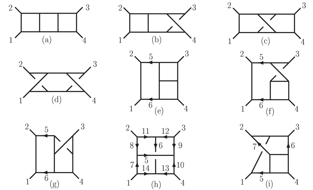
Fig. 10 shows the nine cubic four-point graphs at three loops that do not contain three-point subdiagrams. Both the SYM and supergravity amplitudes can be described by giving the loop-momentum numerator polynomials for these graphs. (A recent, alternate representation [58] makes use of the graphs with three-point subdiagrams, but they are not necessary.) In addition, the SYM graphs are to be multiplied by the corresponding color structure, as in fig. 8. Notice that seven of the nine graphs, (a)–(g), have iterated two-particle cuts, so they can be computed via the rung rule. Only (h) and (i) require additional work.
| Integral | for super-Yang-Mills |
|---|---|
| (a)–(d) | |
| (e)–(g) | |
| (h) | |
| (i) |
Table 2 gives the values of for SYM in terms of the following invariants,
| (58) |
Note that is quadratic in the loop momenta , if , but is linear. Every is manifestly quadratic in the loop momenta, consistent with for . It is easy to verify the numerators for graphs (a)–(g) using the rung rule.
| Integral | for supergravity |
|---|---|
| (a)–(d) | |
| (e)–(g) | |
| (h) | |
| (i) | |
Table 3 gives the values of for supergravity, in a form [27] which is also manifestly quadratic in the loop momenta. (In an earlier version of the amplitude [26], the quadratic nature was not yet manifest.) Comparing the two sets of numerators, we see that the supergravity ones are the squares of the SYM ones, up to contact terms, as expected from the KLT relations. For example, in graphs (e)–(g), , so (modulo terms).
Because the numerator factors for both supergravity and SYM are manifestly quadratic in the loop momenta, the critical dimension at three loops should continue to obey eq. (8), i.e. . Indeed, when the ultraviolet poles in the nine integrals for supergravity are evaluated, no further cancellation is found, and the resulting pole is
| (59) |
corresponding to a counterterm of the form in . (The form of this divergence was recently reproduced from duality arguments in string theory [17]; however, the rational number does not agree with eq. (59) as of this writing. Whether or not this indicates an issue in decoupling massive states [22] remains unclear.)
6 supergravity at four loops
The general strategy [28, 78] used to compute the four-loop four-point amplitude in supergravity is the same as at three loops; however, the bookkeeping issues are considerably greater. One can start by classifying the cubic vacuum graphs. At three loops there were only two; at four loops there are five, shown in fig. 11.
The next step is to decorate the five vacuum graphs with four external legs to get the cubic four-point graphs. As at lower loops, graphs containing triangles (three propagators or fewer on a loop) or other three point subgraphs can be dropped. Fig. 11(a) only gives rise to triangle-containing graphs, so it can be neglected henceforth. Altogether there are 50 cubic four-point graphs with nonvanishing numerators. Graphs (b) and (c) do generate no-triangle four-point graphs, but the numerators for all such graphs can be determined, up to possible contact terms, using the rung rule. For this reason, their associated numerator polynomials are the simplest. Graphs (d), and particularly (e), give rise to the most complex numerators.

The numerators are first determined for SYM using the method of maximal cuts. At four loops the maximal cuts have 13 cut conditions . Then near-maximal cuts with only 12 cut conditions are considered, followed by ones with 11. At this point the SYM ansatz is complete; no more terms need to be added. The result is verified by comparison against many of the generalized cuts with real momenta, shown in fig. 12. Cases (a) and (i) involve six- and seven-point next-to-MHV amplitudes, for which the sums over super-multiplets crossing the cuts are more intricate than when all amplitudes are MHV. These cuts were evaluated using compact results for the super-sums obtained by Elvang, Freedman and Kiermaier [79].

The 50 numerator polynomials for supergravity are then constructed using information provided by the KLT relations. The results are quite lengthy, but are provided as Mathematica readable files in ref. [28], along with some tools for manipulating them.
From the numerator polynomials, the ultraviolet behavior of the amplitude can be extracted. One has to expand the integrals in the limit of small external momenta, relative to the loop momenta [80]. If the ultraviolet behavior is manifest, as at three loops with the representation found in ref. [27], then only the first term in this expansion is required. At four loops, it was necessary to go to third order to see all observed cancellations. More concretely, the numerator polynomials, omitting an overall factor of , have a mass dimension of 12, i.e. each term is of the form , where and stand respectively for external and loop momenta. The maximum value of turns out to be 8, for every integral. The integrals all have 13 propagators, so they have the form . The amplitude is manifestly finite in , because . (This result is not unexpected, given the absence of a counterterm [52, 53].) The amplitude is not manifestly finite in ; to see that requires cancellation of the , and terms, after expansion around small .
The cancellation of the terms is relatively simple; one can set the external momenta to zero, and collect the coefficients of the two resulting vacuum graphs, (d) and (e) in fig. 11, observing that the (d) and (e) coefficients both vanish. The cancellation of the terms (and the terms) is trivial: Using dimensional regularization, with no dimensionful parameter, Lorentz invariance does not allow an odd-power divergence. The most intricate cancellation is of the terms, corresponding to the vanishing of the coefficient of the potential counterterm in . In the expansion of the integrals to the second subleading order as , 30 different four-loop vacuum integrals are generated. However, there are consistency relations between the integrals, corresponding to the ability to shift the loop momenta by external momenta before expanding around . These consistency relations are powerful enough to imply the cancellation of the ultraviolet pole in . As a check, we evaluated all the ultraviolet poles directly, with the same conclusion.
In summary, the four-loop four-point amplitude of supergravity is ultraviolet finite for [28], the same critical dimension as for super-Yang-Mills theory. Finiteness in is a consequence of nontrivial cancellations, beyond those already found at three loops [26, 27]. These results provide the strongest direct support to date for the possibility that supergravity might be a perturbatively finite quantum theory of gravity.
7 Conclusions and Outlook
What are the prospects for going beyond four loops? As mentioned in the Introduction, there are indications of a problem [17, 18, 19] with the pure spinor formalism [15] at five loops, which could lead to a deviation from the critical dimension formula (8) at this order. It would be very interesting to clarify the situation by computing the complete amplitude. This would be a major undertaking, but recent developments might provide some assistance [57, 58, 56]. It is also worth noting that the unitarity method generically implies sets of higher-loop cancellations as a consequence of lower-loop ones [32], by finding the latter contributions as subgraphs exposed by unitarity cuts. The fact that certain higher-loop cancellations were implied by the no-triangle behavior of one-loop -point amplitudes was discussed in section 4, but the excellent ultraviolet behavior of the two-, three- and four-loop four-point amplitudes has similar implications. Combining this information properly is still an issue, however.
The unitarity method works with on-shell objects, so it can maintain more supersymmetry than is generally possible with off-shell Feynman diagrams. However, not all symmetries of supergravity are kept manifest in the current approach. In particular the theory has a continuous noncompact coset symmetry, [1]. The 70 massless scalars parametrize the coset space , and the non- part of the symmetry is realized nonlinearly. When using the KLT relations, there is an symmetry associated with each supersymmetry, so only an subgroup of the linearly-realized is kept manifest, and none of the . There has been some recent progress on the role of in supergravity: using it to construct terms in the light-cone superspace Hamiltonian [81]; describing its explicit action on covariant fields [82]; exploring its implications for tree-level matrix elements [83, 77, 84], and also at loop level [85, 86]; and assessing the invariance of the counterterm [87]. However, a deeper understanding of the implications of invariance would certainly be welcome.
Suppose that supergravity is finite to all loop orders. This still would not prove that it is a nonperturbatively consistent theory of quantum gravity. There are at least two reasons to think that it might need a nonperturbative ultraviolet completion:
- 1.
The (likely) or worse growth of the coefficients of the order terms in the perturbative expansion, which for fixed-angle scattering, means a non-convergent behavior .
- 2.
The fact that the perturbative series seems to be invariant, while the mass spectrum of black holes is non-invariant (see e.g. ref. [88] for recent discussions).
QED is an example of a perturbatively well-defined theory that needs an ultraviolet completion; it also has factorial growth in its perturbative coefficients, , due to ultraviolet renormalons associated with the Landau pole. Of course, for small values of , QED works extremely well; for example, it predicts the anomalous magnetic moment of the electron to 10 digits of accuracy. Also, we know of many pointlike nonperturbative ultraviolet completions for QED, namely asymptotically free grand unified theories. Are there any imaginable pointlike completions for supergravity? Maybe the only completion is string theory; or maybe this cannot happen because of the impossibility of decoupling nonperturbative states [22].
In any event, it is clear that the remarkably good perturbative ultraviolet behavior of supergravity has provided many surprises to date. Although the theory may not be of direct phenomenological interest, perhaps it could some day point the way to other, more realistic finite theories. As a “toy model” for a pointlike theory of quantum gravity, it has been extremely instructive, and is still well worth exploring further.
Acknowledgments
I am grateful to Zvi Bern, John Joseph Carrasco, Henrik Johansson, David Kosower and Radu Roiban for collaboration on many of the topics described here, and to Zvi Bern for comments on the manuscript. I thank the organizers of the 47th International School of Subnuclear Physics for the opportunity to present these lectures in such a stimulating and pleasant environment. This work was supported by the US Department of Energy under contract DE-AC02-76SF00515.
References
- [1] E. Cremmer and B. Julia, Phys. Lett. B 80, 48 (1978); Nucl. Phys. B 159, 141 (1979).
- [2] B. de Wit and D. Z. Freedman, Nucl. Phys. B 130, 105 (1977).
- [3] E. Cremmer, B. Julia and J. Scherk, Phys. Lett. B 76, 409 (1978).
- [4]
S. Weinberg, in Understanding the Fundamental Constituents of
Matter, ed. A. Zichichi (Plenum Press, New York, 1977);
S. Weinberg, in General Relativity, eds. S. W. Hawking and W. Israel
(Cambridge University Press, 1979), p. 700;
M. Niedermaier and M. Reuter, Living Rev. Rel. 9, 5 (2006). - [5] P. Hořava, Phys. Rev. D 79, 084008 (2009) [0901.3775 [hep-th]].
- [6] S. Deser, J. H. Kay and K. S. Stelle, Phys. Rev. Lett. 38, 527 (1977).
- [7] S. Ferrara and B. Zumino, Nucl. Phys. B 134, 301 (1978).
- [8] S. Deser and J. H. Kay, Phys. Lett. B 76, 400 (1978).
- [9] P. S. Howe and U. Lindström, Nucl. Phys. B 181, 487 (1981).
- [10] R. E. Kallosh, Phys. Lett. B 99, 122 (1981).
- [11] Z. Bern, L. J. Dixon, D. C. Dunbar, M. Perelstein and J. S. Rozowsky, Nucl. Phys. B 530, 401 (1998) [hep-th/9802162].
- [12] P. S. Howe and K. S. Stelle, Phys. Lett. B 554, 190 (2003) [hep-th/0211279].
- [13] G. Bossard, P. S. Howe and K. S. Stelle, Gen. Rel. Grav. 41, 919 (2009) [0901.4661 [hep-th]].
- [14] G. Bossard, P. S. Howe and K. S. Stelle, Phys. Lett. B 682, 137 (2009) [0908.3883 [hep-th]].
- [15] N. Berkovits, Phys. Rev. Lett. 98, 211601 (2007) [hep-th/0609006].
- [16] M. B. Green, J. G. Russo and P. Vanhove, Phys. Rev. Lett. 98, 131602 (2007) [hep-th/0611273].
- [17] M. B. Green, J. G. Russo and P. Vanhove, 1002.3805 [hep-th].
- [18] P. Vanhove, 1004.1392 [hep-th].
- [19] J. Björnsson and M. B. Green, 1004.2692 [hep-th].
- [20] R. Kallosh, Phys. Rev. D 80, 105022 (2009) [0903.4630 [hep-th]].
- [21]
G. Chalmers,
hep-th/0008162;
M. B. Green, J. G. Russo and P. Vanhove, JHEP 0702, 099 (2007) [hep-th/0610299]. - [22] M. B. Green, H. Ooguri and J. H. Schwarz, Phys. Rev. Lett. 99, 041601 (2007) [0704.0777 [hep-th]].
- [23] Z. Bern, J. J. M. Carrasco, H. Johansson, to appear in the Proceedings of the 46th International School of Subnuclear Physics [0902.3765 [hep-th]].
- [24] Z. Bern, L. J. Dixon, D. C. Dunbar and D. A. Kosower, Nucl. Phys. B 425, 217 (1994) [hep-ph/9403226]; Nucl. Phys. B 435, 59 (1995) [hep-ph/9409265].
- [25] H. Kawai, D. C. Lewellen and S. H. H. Tye, Nucl. Phys. B 269, 1 (1986).
- [26] Z. Bern, J. J. Carrasco, L. J. Dixon, H. Johansson, D. A. Kosower and R. Roiban, Phys. Rev. Lett. 98, 161303 (2007) [hep-th/0702112].
- [27] Z. Bern, J. J. M. Carrasco, L. J. Dixon, H. Johansson and R. Roiban, Phys. Rev. D 78, 105019 (2008) [0808.4112 [hep-th]].
- [28] Z. Bern, J. J. Carrasco, L. J. Dixon, H. Johansson and R. Roiban, Phys. Rev. Lett. 103, 081301 (2009) [0905.2326 [hep-th]].
- [29] Z. Bern, L. J. Dixon, M. Perelstein and J. S. Rozowsky, Nucl. Phys. B 546, 423 (1999) [hep-th/9811140].
- [30]
Z. Bern, N. E. J. Bjerrum-Bohr and D. C. Dunbar,
JHEP 0505, 056 (2005)
[hep-th/0501137];
N. E. J. Bjerrum-Bohr, D. C. Dunbar and H. Ita, Phys. Lett. B 621, 183 (2005) [hep-th/0503102]. - [31] N. E. J. Bjerrum-Bohr, D. C. Dunbar, H. Ita, W. B. Perkins and K. Risager, JHEP 0612, 072 (2006) [hep-th/0610043].
- [32] Z. Bern, L. J. Dixon and R. Roiban, Phys. Lett. B 644, 265 (2007) [hep-th/0611086].
- [33]
S. Mandelstam,
Nucl. Phys. B 213, 149 (1983);
P. S. Howe, K. S. Stelle and P. K. Townsend, Nucl. Phys. B 214, 519 (1983);
L. Brink, O. Lindgren and B. E. W. Nilsson, Phys. Lett. B 123, 323 (1983). - [34] G. ’t Hooft and M. J. G. Veltman, Annales Poincare Phys. Theor. A 20, 69 (1974).
- [35] M. H. Goroff and A. Sagnotti, Phys. Lett. B 160, 81 (1985); Nucl. Phys. B 266, 709 (1986).
- [36] A. E. M. van de Ven, Nucl. Phys. B 378, 309 (1992).
- [37] M. T. Grisaru, Phys. Lett. B 66, 75 (1977).
- [38] E. Tomboulis, Phys. Lett. B 67, 417 (1977).
- [39] P. van Nieuwenhuizen and C. C. Wu, J. Math. Phys. 18, 182 (1977).
- [40]
M. T. Grisaru, H. N. Pendleton and P. van Nieuwenhuizen,
Phys. Rev. D 15, 996 (1977);
M. T. Grisaru and H. N. Pendleton, Nucl. Phys. B 124, 81 (1977). - [41] J. H. Schwarz, Phys. Rept. 89, 223 (1982).
- [42]
I. Robinson, unpublished;
L. Bel, Acad. Sci. Paris, Comptes Rend. 247, 1094 (1958) and 248, 1297 (1959). - [43] D. J. Gross and E. Witten, Nucl. Phys. B 277, 1 (1986).
- [44] M. B. Green, J. H. Schwarz and L. Brink, Nucl. Phys. B 198, 474 (1982).
- [45] Z. Bern, J. S. Rozowsky and B. Yan, Phys. Lett. B 401, 273 (1997) [hep-ph/9702424].
- [46] N. Marcus and A. Sagnotti, Nucl. Phys. B 256, 77 (1985).
- [47] A. Galperin, E. Ivanov, S. Kalitsyn, V. Ogievetsky and E. Sokatchev, Class. Quant. Grav. 1, 469 (1984); Class. Quant. Grav. 2, 155 (1985).
- [48] Z. Bern, L. J. Dixon and V. A. Smirnov, Phys. Rev. D 72, 085001 (2005) [hep-th/0505205].
- [49] Z. Bern, M. Czakon, L. J. Dixon, D. A. Kosower and V. A. Smirnov, Phys. Rev. D 75, 085010 (2007) [hep-th/0610248].
- [50] Z. Bern, J. J. M. Carrasco, H. Johansson and D. A. Kosower, Phys. Rev. D 76, 125020 (2007) [0705.1864 [hep-th]].
- [51] H. Elvang, D. Z. Freedman and M. Kiermaier, 1003.5018 [hep-th].
- [52] J. M. Drummond, P. J. Heslop, P. S. Howe and S. F. Kerstan, JHEP 0308, 016 (2003) [hep-th/0305202].
- [53] R. Kallosh, JHEP 0909, 116 (2009) [0906.3495 [hep-th]].
- [54] L. J. Dixon, in QCD & Beyond: Proceedings of TASI ’95, ed. D. E. Soper (World Scientific, 1996) [hep-ph/9601359].
- [55]
Z. Bern, A. De Freitas and H. L. Wong,
Phys. Rev. Lett. 84, 3531 (2000)
[hep-th/9912033];
N. E. J. Bjerrum-Bohr and K. Risager, Phys. Rev. D 70, 086011 (2004) [hep-th/0407085];
N. E. J. Bjerrum-Bohr and O. T. Engelund, 1002.2279 [hep-th]. - [56] Z. Bern, T. Dennen, Y. t. Huang and M. Kiermaier, 1004.0693 [hep-th].
- [57] Z. Bern, J. J. M. Carrasco and H. Johansson, Phys. Rev. D 78, 085011 (2008) [0805.3993 [hep-ph]].
- [58] Z. Bern, J. J. M. Carrasco and H. Johansson, 1004.0476 [hep-th].
- [59]
J. M. Maldacena,
Adv. Theor. Math. Phys. 2, 231 (1998)
[Int. J. Theor. Phys. 38, 1113 (1999)]
[hep-th/9711200];
S. S. Gubser, I. R. Klebanov and A. M. Polyakov, Phys. Lett. B 428, 105 (1998) [hep-th/9802109];
O. Aharony, S. S. Gubser, J. M. Maldacena, H. Ooguri and Y. Oz, Phys. Rept. 323, 183 (2000) [hep-th/9905111]. - [60]
L. D. Landau,
Nucl. Phys. 13, 181 (1959);
S. Mandelstam, Phys. Rev. 115, 1741 (1959);
R. E. Cutkosky, J. Math. Phys. 1, 429 (1960). - [61]
Z. Bern and A. G. Morgan,
Nucl. Phys. B 467, 479 (1996)
[hep-ph/9511336];
Z. Bern, L. J. Dixon, D. C. Dunbar and D. A. Kosower, Phys. Lett. B 394, 105 (1997) [hep-th/9611127]. - [62]
Z. Bern, L. J. Dixon and D. A. Kosower,
JHEP 0001, 027 (2000)
[hep-ph/0001001];
JHEP 0408, 012 (2004) [hep-ph/0404293]. - [63] Z. Bern, L. J. Dixon and D. A. Kosower, Nucl. Phys. B 513, 3 (1998) [hep-ph/9708239].
- [64]
R. Britto, F. Cachazo and B. Feng,
Nucl. Phys. B 715, 499 (2005)
[hep-th/0412308];
R. Britto, F. Cachazo, B. Feng and E. Witten, Phys. Rev. Lett. 94, 181602 (2005) [hep-th/0501052]. - [65]
Z. Bern, L. J. Dixon and D. A. Kosower,
Phys. Rev. D 73, 065013 (2006)
[hep-ph/0507005];
C. F. Berger, Z. Bern, L. J. Dixon, D. Forde and D. A. Kosower, Phys. Rev. D 74, 036009 (2006) [hep-ph/0604195]. - [66] G. Ossola, C. G. Papadopoulos and R. Pittau, Nucl. Phys. B 763, 147 (2007) [hep-ph/0609007]; JHEP 0803, 042 (2008) [0711.3596 [hep-ph]]; JHEP 0805, 004 (2008) [0802.1876 [hep-ph]].
- [67]
R. K. Ellis, W. T. Giele and Z. Kunszt,
JHEP 0803, 003 (2008)
[0708.2398 [hep-ph]];
W. T. Giele, Z. Kunszt and K. Melnikov, JHEP 0804, 049 (2008) [0801.2237 [hep-ph]];
W. T. Giele and G. Zanderighi, JHEP 0806, 038 (2008) [0805.2152 [hep-ph]]. - [68] C. F. Berger et al., Phys. Rev. D 78, 036003 (2008) [0803.4180 [hep-ph]].
- [69] C. F. Berger and D. Forde, 0912.3534 [hep-ph].
- [70] R. J. Eden, P. V. Landshoff, D. I. Olive and J. C. Polkinghorne, The Analytic S Matrix (Cambridge University Press, 1966).
- [71] Z. Bern, V. Del Duca, L. J. Dixon and D. A. Kosower, Phys. Rev. D 71, 045006 (2005) [hep-th/0410224].
- [72] R. Britto, F. Cachazo and B. Feng, Nucl. Phys. B 725, 275 (2005) [hep-th/0412103].
- [73]
E. I. Buchbinder and F. Cachazo,
JHEP 0511, 036 (2005)
[hep-th/0506126];
F. Cachazo and D. Skinner, 0801.4574 [hep-th];
F. Cachazo, 0803.1988 [hep-th];
F. Cachazo, M. Spradlin and A. Volovich, Phys. Rev. D 78, 105022 (2008) [0805.4832 [hep-th]];
M. Spradlin, A. Volovich and C. Wen, Phys. Rev. D 78, 085025 (2008) [0808.1054 [hep-th]]. - [74] S. J. Parke and T. R. Taylor, Phys. Rev. Lett. 56, 2459 (1986).
- [75]
W. Siegel,
Phys. Lett. B 84, 193 (1979);
Z. Bern and D. A. Kosower, Nucl. Phys. B 379, 451 (1992);
Z. Bern, A. De Freitas, L. J. Dixon and H. L. Wong, Phys. Rev. D 66, 085002 (2002) [hep-ph/0202271]. - [76] N. E. J. Bjerrum-Bohr and P. Vanhove, JHEP 0804, 065 (2008) [0802.0868 [hep-th]]; JHEP 0810, 006 (2008) [0805.3682 [hep-th]]; Fortsch. Phys. 56, 824 (2008) [0806.1726 [hep-th]].
- [77] N. Arkani-Hamed, F. Cachazo and J. Kaplan, 0808.1446 [hep-th].
- [78] Z. Bern, J. J. M. Carrasco, L. J. Dixon, H. Johansson and R. Roiban, to appear.
- [79] H. Elvang, D. Z. Freedman and M. Kiermaier, JHEP 0904, 009 (2009) [0808.1720 [hep-th]]; and private communication.
- [80]
A. A. Vladimirov,
Theor. Math. Phys. 43, 417 (1980)
[Teor. Mat. Fiz. 43, 210 (1980)];
N. Marcus and A. Sagnotti, Nuovo Cim. A 87, 1 (1985). - [81] L. Brink, S. S. Kim and P. Ramond, JHEP 0806, 034 (2008) [0801.2993 [hep-th]].
- [82] R. Kallosh and M. Soroush, Nucl. Phys. B 801, 25 (2008) [0802.4106 [hep-th]].
- [83] M. Bianchi, H. Elvang and D. Z. Freedman, JHEP 0809, 063 (2008) [0805.0757 [hep-th]].
- [84] R. Kallosh and T. Kugo, JHEP 0901 (2009) 072 [0811.3414 [hep-th]].
- [85] R. Kallosh, C. H. Lee and T. Rube, JHEP 0902 (2009) 050 [0811.3417 [hep-th]].
- [86] S. He and H. Zhu, 0812.4533 [hep-th].
- [87] J. Brödel and L. J. Dixon, JHEP 1005, 003 (2010) [0911.5704 [hep-th]].
- [88] M. Bianchi, S. Ferrara and R. Kallosh, 0910.3674 [hep-th]; JHEP 1003, 081 (2010) [0912.0057 [hep-th]].