CMB power spectra from cosmic strings: predictions
for the Planck satellite and beyond

In CMB power spectra calculations for inflationary models with cosmic strings, the inflationary contribution is essentially uncorrelated with the cosmic string contribution. This is because the inflationary perturbations are laid down by an independent field $60$ e-foldings before the strings are formed, and because the complex string dynamics rapidly destroys correlations with earlier times (see Sec. III.3). As a result we may write the total spectrum $\ell(\ell+1)\mathcal{C}_{\ell}$ as a sum of two independent spectra and take the cross-correlation term to be negligible:

where $\mathcal{C}_{\ell}^{\mathrm{inf}}$ is the inflationary contribution and $\mathcal{C}_{\ell}^{\mathrm{str}}$ is the string contribution. We can use standard methods [51] to determine $\mathcal{C}_{\ell}^{\mathrm{inf}}$ and it is therefore upon $\mathcal{C}_{\ell}^{\mathrm{str}}$ that this article is focused.

Physically the strings cause CMB anisotropies by creating perturbations in the space-time metric, which are roughly of the same order as $G\mu$, where $\mu$ is the string mass per unit length, $G$ is the gravitational constant, and $G\mu\lesssim 10^{-6}$ to be consistent with current observations [3]. These inhomogeneities in the metric then lead to perturbations in the matter and radiation that themselves evolve and influence the strings, but we can neglect this back-reaction since the resulting perturbations of the strings would then result in changes only of order $(G\mu)^{2}$ to the metric.

In order to determine the string contribution to a two-point correlation function, such as the CMB temperature power spectrum, we are required to solve a set of linear differential equations of the following form, in which the string energy-momentum tensor components act as source terms $\tilde{S}_{a}$:

Here $X_{a}$ is the quantity of interest and $\tilde{X}_{a}$ its Fourier transform, while $\hat{\mathcal{D}}_{ac}$ is a differential operator, dependent upon the cosmic scale factor $a$, the background matter density $\rho$ and similar quantities. Our notation is such that $\tau$ is the conformal time and $\mathbf{k}$ is the comoving wavevector. The homogeneous version of this equation $(\tilde{S}_{c}=0)$, which corresponds to the inflationary case, can be solved by standard codes and therefore, in principle, we may use a Green’s function $\mathcal{G}_{ac}(k,\tau_{0},\tau)$ to give the power spectrum at conformal time $\tau_{0}$ for the string case via:

Hence the data required to calculate such two-point correlation functions are the two-point unequal-time correlators of the string energy-momentum tensor components [33, 18]:

Note that statistical isotropy implies that $\tilde{U}_{ab}$ is not dependent on the direction of $\mathbf{k}$ and further that it is real-valued.

Significant simplification in the form of $\tilde{U}_{ab}$ may be made using the scaling property, briefly mentioned in the introduction. Under scaling, any statistical measure of the spatial distribution of strings scales with the horizon size, which is just $\tau$ in comoving coordinates. For example the comoving length-density of string is $\alpha/\tau^{2}$, where $\alpha$ is a dimensionless constant. The existence of this attractor was predicted by Kibble [34] and has been confirmed in Nambu-Goto simulations [39, 45, 52] (with some assumptions about the decay of loops) and in Abelian Higgs simulations [49, 53, 23]. We will present further evidence in support of scaling in our results section.

The power of scaling is that it enables us to write $\tilde{U}_{ab}$ in terms of a function of just two variables:

Here $\phi_{0}$ sets the energy-scale of the problem and converts between the scaling spatial distribution of string and the distribution of energy. For example, in the case of the Abelian Higgs model (see next section) it is the vacuum expectation value of the scalar field. The comoving simulation volume $V$ appears here because we define our Fourier transform so that it leaves dimensions unchanged:

The UETC scaling function $\tilde{C}_{ab}$ can be seen to allow data to be taken for very large $k$ at small $\tau$ and $\tau^{\prime}$ and then used to provide information about small $k$ at large $\tau$ and $\tau^{\prime}$. This is critical for the present calculations, as noted in the introduction.

Further power of the UETC scaling functions derives from their functional form: they decay for large and small time ratios $\tau/\tau^{\prime}$, and for large $k\sqrt{\tau\,\tau^{\prime}}$ (small scales), while causality constrains their form at low $k\sqrt{\tau\,\tau^{\prime}}$. This crucially means that we need study a scaling network for only a relatively short range of times and in a limited simulation volume. However as noted in the introduction, small length scales become more important when considering small angular scales (see next section).

While our approach is to measure $\tilde{C}_{ab}$ from cosmic string simulations, and therefore find $\tilde{U}_{ab}$, we do not in fact then use Eq. (3). Instead we decompose $\tilde{C}_{ab}$ into a sum over products as [54]:

The problem then breaks down to:

where:

In practice we do not calculate this integral via a Green’s function, but instead apply a modified version of CMBEASY [55] to determine the CMB power spectrum contribution from the coherent active source $\tilde{c}_{nb}/\sqrt{\tau}$.

In principle there are 55 possible UETCs between the 4 scalar, 4 vector and 2 tensor degrees of freedom in the energy-momentum tensor $\tilde{T}_{\mu\nu}$, but thanks to statistical isotropy and energy conservation, we in fact need only to measure 5 scaling functions [56]. The scalar UETCs that we calculate involve projections from $\tilde{T}_{\mu\nu}$ that, via Einstein’s equations, directly source the two Bardeen potentials [57]:

From these projections there are 3 independent UETC scaling functions that we must measure:

Then in the tensor case we project out the two tensor degrees of freedom (see BHKU), which we denote as $\tilde{S}^{\mathrm{T1}}$ and $\tilde{S}^{\mathrm{T2}}$. We then determine:

where the factor of $2$ is present to ensure that $\tilde{C}\!\!\stackrel{{\scriptstyle\scriptstyle{\mathrm{T}}}}{{{}_{\!}}}$ matches the definition of Ref. [19].

Following Ref. [19], we make a change in the scaling function definition when considering the two vector degrees of freedom from $\tilde{T}_{0i}$, $\tilde{S}^{\mathrm{V1}}$ and $\tilde{S}^{\mathrm{V2}}$ (see BHKU). Specifically we pull out a factor of $k^{2}\tau\tau^{\prime}$ from the scaling function such that:

This definition is motivated by the fact that covariant energy-momentum conservation requires that the vector UETC varies as $k^{2}$ at small $k$ while the other UETCs that we measure tend to a constant value as $k\rightarrow 0$; and it is desirable for all UETC scaling functions to have the same super-horizon properties.

However, it should be noted that the above discussion requires a small change because scaling is broken near the time of radiation-matter equality $\tau_{\mathrm{eq}}$, since $\tau_{\mathrm{eq}}$ is a second dimensional scale which enters the problem. We hence are required to take UETC data in both the radiation and matter eras — although the matter era data dominates the CMB results — and we then use interpolation in order to model the transition. Scaling is also broken as the Universe enters the current accelerating phase, causing the string density to decay, which we model by partially suppressing the stress source.

For more details of the solution of the linearized Einstein-Boltzmann equations in the presence of sources see Refs. [59, 58].

For computational speed, we simulate local cosmic strings by solving the classical field equations of the simplest theory that contains them: the Abelian Higgs model. In the notation of BHKU this has Lagrangian density:

with $D_{\mu}=\partial_{\mu}+iA_{\mu}$ and $F_{\mu\nu}=\partial_{\mu}A_{\nu}-\partial_{\nu}A_{\mu}$ while $e$ and $\lambda$ are dimensionless coupling constants. In a spatially flat Friedmann-Robertson-Walker(FRW) metric with scale factor $a$, this leads to the following Euler-Lagrange equations:

where the gauge choice $A_{0}=0$ has been made. Here we use over-dots to denote differentiation with respect to conformal time $\tau$, while $\partial_{i}$ denotes differentiation with respect to comoving Cartesian coordinates.

When simulating this model in an expanding universe, the simulations must resolve the comoving string width $w_{0}/a$ (i.e. $w_{0}$ is the fixed physical width $\sim\phi_{0}^{-1}$). They must also contain at least one horizon volume of comoving diameter $2\tau$. However, these two scales diverge rapidly, with their ratio growing as $\tau^{3}$ in the matter era, while we require ratios $\gtrsim 100$ in order for strings to scale. Hence with $1024^{3}$ lattice simulations, which are the largest that are practical with our available facilities, we cannot study a scaling network using these equations for long enough to measure the UETCs up to sufficiently high $\tau/\tau^{\prime}$ ratios. Furthermore, the increase in this ratio with computer time $t_{\mathrm{cpu}}$ varies as $t_{\mathrm{cpu}}\!\!\!\!\!\!\!^{1/12}$ and hence the returns from much larger outlays are minimal. In BHKU we therefore proceeded by allowing temporal variations in the coupling constants $\lambda$ and $e$:

such that the comoving string width now varies as

where $s$ is the string width control parameter. If $s=0$, then the factors of $a$ on the right-hand-side of Eqs. (18)-(20) are removed and the string width remains constant in comoving coordinates, while $s=1$ gives the normal dynamics of the model. Note that the above dependencies preserve the ratio $\lambda/2e^{2}$, which we set to be unity for the simulations described in this article: the Bogomol’nyi limit [60].

Simply evolving the above dynamical equations (Eqs. 18 and 19) while varying $\lambda$ and $e$ will not preserve the constraint Eq. (20). Hence the BHKU method is to vary the model action with respect to the fields whilst allowing for the temporal dependence in $\lambda$ and $e$, which then yields a consistent set of dynamical and constraint equations: Eqs. (18) and (20) in addition to a modified form of Eq. (19):

However, for $s\neq 1$ the action is no longer a 4-scalar and hence there is a breach of covariant energy conservation. Since it is the energy-momentum tensor that seeds the cosmological perturbations which result from strings, then this is clearly a potential problem. Fortunately in BHKU it was established that the effects on the UETCs, and therefore the CMB power spectra, are minimal on the relevant scales, but we present additional evidence in support of this approach in the next section.

As has already been alluded to, for strings to scale their width must be much less than their separation, which is of order the horizon size. This statement may be made more precise by introducing the (comoving) network length scale $\xi$, defined by:

where $L$ is the comoving string length¹¹ 1 We measure $L$ by detecting the lattice grid-squares around which the phase $\phi$ has a net winding (using the gauge-invariant method of Ref. [61]) and then we approximately reconstruct the string path as a collection of perpendicular segments of length $\Delta x$ passing through these squares. We then apply the Scherrer-Vilenkin correction factor of $\pi/6$ [62] in order to approximately account for over-estimate due to representing a smooth path by perpendicular segments (see Ref. [50] for more discussion). in the simulation volume $V$. We observe in our simulations that accurate scaling sets in at $\xi\gtrsim 40w$ whereupon $\xi\sim 0.3\tau$.

However, in BHKU we were limited to an Abelian Higgs simulation size of $512^{3}$, which is about the minimum required to study a scaling network of strings. We therefore were forced to be content with initial conditions that yielded not $\xi\propto\tau$ but $\xi\propto(\tau-\tau_{\xi=0})$, as shown in Fig. 1, were $\tau_{\xi=0}$ is negative. That is, at early times string decay occurred more quickly than scaling would have predicted and $\xi$ increased rapidly, but then stabilized to an approximately constant $\mathrm{d}\xi/\mathrm{d}\tau$ once $\xi\gtrsim 40w$ (where $w\approx\phi_{0}^{-1}$ but is slowly decreasing with $\tau$ in the $s=0.3$ simulation for which BHKU-style results are plotted). As can be seen in the figure, this rapid increase aids the creation of an approximately scaling network for simulations that are causally limited to small times, albeit scaling with $(\tau-\tau_{\xi=0})$ rather than $\tau$. Fortunately, at times of cosmological interest we have $\tau\gg\tau_{\xi=0}$ and therefore this offset is not actually relevant. Furthermore, when $\tau$ was replaced by $(\tau-\tau_{\xi=0})$ in the calculations of the UETC scaling functions, the equal-time scaling functions $\tilde{C}(k\tau,1)$ were seen to be approximately constant in $\tau$, as is required for scaling.

Despite the success of the $(\tau-\tau_{\xi=0})$ replacement when using the BHKU initial conditions, with the larger $1024^{3}$ simulations available for the present work we noted a slow drift in the $\mathrm{d}\xi/\mathrm{d}\tau$ value, even at late times. Further, there was a slow rise in the magnitude of the $\tau_{\xi=0}$-corrected equal-time scaling functions. This is expected at some level since the dynamical equations contain the quantity:

where $n$ is unity for the radiation era and 2 for the matter era. The ratio of this damping scale $\tau/n$ to the network length scale $\xi$ changes with time if $\tau_{\xi=0}\neq 0$ and at $\tau\sim|\tau_{\xi=0}|$ with negative $\tau_{\xi=0}$, the system has a lower than asymptotic value of $\tau/n\xi$ — it is being damped too heavily. We hence now employ initial conditions that yield (effectively) $\tau_{\xi=0}=0$, although now we do not see scaling until long after the causal run-time limit of our previous $512^{3}$ simulations.

In principle, the initial conditions for the fields are set by their fluctuations (quantum or thermal) at string formation, which have a finite, microscopic, correlation length (see e.g. [63]). Fortunately the string network is observed to relax to scaling for a wide variety of initial conditions and so it is not important to model the initial fluctuations precisely. In BHKU we employed initial conditions that were designed to model a vacuum phase transition at the end of inflation: each lattice site was given an independent phase for $\phi$, with $|\phi|=\phi_{0}$, and the initial time $\tau_{\mathrm{start}}$ was set roughly equal to the lattice spacing $\Delta x$. The gauge field and the canonical momentum $\dot{\phi}$ were set to zero. However, that set of initial conditions means that the simulations begin with $\tau_{\mathrm{start}}\sim w$ and this was seen in BHKU to be responsible for the initial rise in $\xi$.

In this work we begin with $\phi$ as a Gaussian random field with correlation length $l_{\phi}$ such that $l_{\phi}\sim\tau_{\mathrm{start}}\gg w$. We are free to choose the two-point auto-correlation function of this Gaussian random field, subject to the constraints that it is zero outside the causal horizon and that its Fourier transform (the power spectrum) must be non-negative. For simplicity we relax the first constraint slightly and opt for:

This decays so rapidly outside the horizon that it is effectively causal with horizon size $\sim l_{\phi}$. We hence generate a field in Fourier space with spectrum $\tilde{P}$ and random phases for each $\mathbf{k}$-mode, before transforming it to real space to become our initial $\phi$ configuration. This gives $\left<\phi^{*}\phi\right>=P_{0}$, which we take as $\phi_{0}^{2}$ since the field should be close to its vacuum except at lattice sites very near to the strings. Further, since Hubble damping at $\tau\gg w$ is too weak to rapidly relax the fields into a network of string, we now employ diffusive (first-order) evolution until a time $\tau_{\mathrm{diff}}$ in order to achieve that. We then have three parameters $\tau_{\mathrm{start}}$, $\tau_{\mathrm{diff}}$ and $l_{\phi}$ which we may vary in order to achieve our goal of $\tau_{\xi=0}=0$, although each test of a point in this 3-dimensional parameter space is very computationally-expensive.

While in principle this $\tau_{\xi=0}\rightarrow 0$ optimization should be performed for each value of $s$, the insensitivity of the string dynamics to changes in $s$ (as noted in BHKU) implies that this computationally-costly process can be performed only once. However, to keep the same settings for these 3 parameters at all $s$ values, we must use a lower lattice spacing $\Delta x$ at higher $s$ in order for strings to still be resolved ($w_{0}/a^{s}>2\Delta x$) at the end of the simulation $\tau=N\Delta x/2$, which is the causal time limit²² 2 We continue the simulations slightly beyond the strict causal limit, since they do not feel the periodic boundary conditions immediately, but the further reduction in string width is not sufficient to greatly affect the reliability of the simulations.. This implies that the accessible $\tau/\tau^{\prime}$ range narrows as $s$ is increased.

The results for $\xi$ from these new initial conditions can be seen in Fig. 1, for simulations in the matter era using $s=0$ (with $a=1$, $\lambda=2$ and $e=1$ during diffusive evolution and $\Delta x=0.5\phi_{0}^{-1}$). Further, we show from the same simulations examples of the equal-time scaling functions $\tilde{C}(k\tau,1)$ in Fig. 2, which provide a scale-dependent test of scaling and is the quantity that is most important for the CMB calculations. These results exhibit scaling on large and intermediate scales to a good degree of accuracy over a ratio in conformal time of 2. A breach of scaling is evident at small-scales, where statistical uncertainties are highly suppressed, but as noted in the introduction this is expected due to the proximity of the associated length scales to the string width. We discuss this issue and our solution to it in Sec. III.4. Numerical results for the string length density under scaling are also given in Table 1 (see also Sec. IV.1.2).

In addition to ensuring that the simulations are exhibiting scaling, we must also check that the use of $s<1$ in our dynamical equations does not introduce significant systematic errors in our UETC scaling function results. This is most readily illustrated using the equal-time case again, with results shown in Fig. 3. We can resolve no dependence upon $s$, except for at high $k\tau$, which is again due to the proximity of the corresponding length scales to the string width. Since the affected scales are the very ones for which we apply the extrapolation mentioned in the introduction, then this effect is of no concern (see Sec. III.4). For completion, however, the $s$-dependence on these scales can be explained as follows. The higher $s$, the more rapid the reduction in comoving string width during the Hubble phase and therefore the attenuation of small scale power (see Sec. III.4) manifests itself at higher $k\tau$. Hence the $s=0$ case yields lower results at the highest-plotted $k\tau$ values.

Since $s=0$ simulations enable the greatest range in $\tau/\tau^{\prime}$ under scaling, while accurately matching the dynamics seen at higher $s$ values, our final CMB results will be based upon $s=0$ simulations and we will limit our remaining discussion in this article to simulations at this value of $s$.

Despite our improved initial conditions, we are only able to study the system when it is scaling accurately for conformal time ratios $\tau/\tau^{\prime}\sim 2$ (corresponding to physical time ratios $\sim 4$ in the radiation era and $\sim 8$ in the matter era). As can be seen in Fig. 4 this is sufficient to map out the important region of the UETCs, and to permit extrapolation in $\tau/\tau^{\prime}$ as explained below. It can be seen that the auto-correlator scaling functions peak for $\tau=\tau^{\prime}$ and decay for unequal times, with decay occurring for $\tau/\tau^{\prime}$ ratios that deviate only slightly from one if $k\sqrt{\tau\tau^{\prime}}$ is large but more slowly on super-horizon scales. In the cross-correlation case $\tilde{C}^{\mathrm{S}}_{12}$, this is broadly true but the peak is noticeably offset on super-horizon scales.

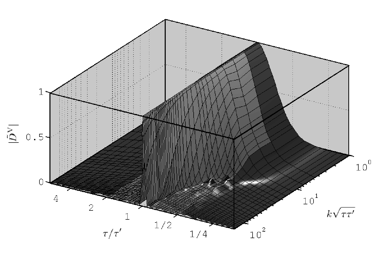
This behaviour can be considered in more detail via the coherence function, which we also use for $\tau/\tau^{\prime}$ extrapolation. We define this function as follows in order to remove the equal-time $k\tau$ dependence from the unequal-time results:

where the modulus in the square-root is relevant only for $\tilde{C}^{\mathrm{S}}_{12}$. This has the attractive feature of being equal to $\pm 1$ at equal-times and is positive at such times for all auto-correlations. Our results are shown in Fig. 5, Fig. 6, and also in Fig. 9. The small-scale behaviour can be understood by considering that the network can quickly decohere when coarse-grained on sub-horizon scales $1/k\ll\xi$ since the relativistic strings must simply travel $\sim 2\pi/k$. As a result the coherence function decays by $|k\tau-k\tau^{\prime}|\sim 2\pi$. Figure 6 highlights this decay, and that the form of $\tilde{D}$ as a function of $k(\tau-\tau^{\prime})$ is scale-independent on small scales. On the other hand, when plotted as a function of $\tau/\tau^{\prime}$, as in Fig. 5, the equal-time ridge becomes increasingly sharp on these scales.

On super-horizon scales the decay is much slower, taking of order a Hubble time: $\tau/\tau^{\prime}\sim 2$. For these longer wave modes the coarse-grained regions each contain a number of horizon volumes. A particular horizon volume that is initially over-dense will become under-dense due to the stochastic string dynamics in a time that is of the same order its initial size, i.e. $\sim\tau^{\prime}$. Therefore the averaged properties of the large coarse-grained region decohere on this time-scale and the decoherence functions for large scales show decay at a fixed value of $\tau/\tau^{\prime}$, independent of scale.

We extrapolate our UETC scaling function results to greater time ratios in the auto-correlation cases by first noting that the form of the coherence function at fixed $k\sqrt{\tau\tau^{\prime}}$ is approximately Gaussian in $\log(\tau/\tau^{\prime})$, but with the width dependent on $k\sqrt{\tau\tau^{\prime}}$. For super- and near-horizon scales we hence take each $k\sqrt{\tau\tau^{\prime}}$ value in turn and match a Gaussian profile $\exp[-\log^{2}(\tau/\tau^{\prime})/2\sigma^{2}]$ to the data at the most extreme $\tau/\tau^{\prime}$ value and then use that profile to extrapolate to larger time ratios. On the other hand, for sub-horizon scales the decay is very rapid and we simply extrapolate with zeros. The results of these extrapolations can be seen in Figs. 4 and 5.

For the cross-correlator $\tilde{C}^{\mathrm{S}}_{12}$ on the other hand, our results show that the $\tau/\tau^{\prime}$-profile on horizon and super-horizon scales is complex and non-Gaussian, making reliable extrapolation impossible. For this correlator we use the Gaussian fits to $\tilde{C}^{\mathrm{S}}_{11}$ and $\tilde{C}^{\mathrm{S}}_{22}$, with widths $\sigma_{11}$ and $\sigma_{22}$, to provide information on the likely decay timescale. We then fit a Gaussian of width $\sigma_{12}=(\sigma_{11}+\sigma_{22})/2$ but with free mean and normalization to the $\tilde{C}^{\mathrm{S}}_{12}$ data from the most extreme time ratios, and then employ that to yield extrapolation.

Figure 7 shows a plot of $k\tau\tilde{C}^{\mathrm{S}}_{11}$ for $\tau^{\prime}=\tau$ from simulations with $s=0$. From the upper pane it can be seen that this quantity is approximately independent of $k\tau$ on sub-horizon scales until $k\tau\sim 200$ at the earliest time shown or until about $k\tau\sim 400$ at the latest time plotted. The plateau highlights an important point: that $\tilde{C}^{\mathrm{S}}_{11}$ drops off as $\approx 1/k\tau$ on sub-horizon scales, which matches our basic expectations as well as similar measures from NG simulations [64]. However, on smaller scales there is a sudden attenuation of power, and at a $k\tau$ value that is increasing with time. The lower pane clarifies the later by re-plotting this against $k$ rather than $k\tau$, showing that this is occurring at a fixed comoving scale of $k\approx 2\phi_{0}$. This corresponds to a few times the string width, which is a fixed comoving width in this $s=0$ simulation.

We find evidence that all equal-time scaling functions vary as approximately $1/k\tau$ on small scales (except in the vector case for which $(k\tau)^{2}\tilde{C}\!\!\stackrel{{\scriptstyle\scriptstyle{\mathrm{V}}}}{{{}_{\!\!}}}$ varies roughly as $1/k\tau$). Figure 8 shows power-law fits to $k\tau\tilde{C}$ (and $(k\tau)^{3}\tilde{C}$ in the vector case) over the range $k\tau=30\rightarrow 100$, which lies between the interesting effects on horizon-scales and the artifacts of the string width on very small-scales. While it would be desirable to have a further order of magnitude via which to confirm the behavior in this regime, it is clear in all cases that a substantial improvement in our estimate of the scaling functions on small scales would be arrived at by extrapolating this trend down to scales near and below the string width.

We extrapolate the unequal time scaling functions to small scales using our knowledge of the attenuation experienced at equal-times for both $\tau$ and $\tau^{\prime}$. First we define the attenuation level $R$ as the ratio of the extrapolated equal-time scaling function and the measured version at time $\tau$:

where we have added a subscript to $\tilde{C}$ to indicate that the measured correlator does not scale exactly and so is not only dependent upon $k\tau$, while $p$ and $Q$ are constants found from the power-law fit. We then extrapolate the UETC scaling function as:

This is based on the correlators being quadratic quantities and includes an appropriate compensation factor for each of the two times involved, which in practice must be nearly equal for the scaling function to be significant, while in the equal-time case this simply returns the power-law fit.

As explained in Sec. II, having determined the UETC scaling functions $\tilde{C}(k\sqrt{\tau\tau^{\prime}},\tau/\tau^{\prime})$, we decompose them into a sum of terms involving functions of a single variable $\tilde{c}_{n}(k\tau)$, which then act as the sources of metric perturbations in the CMB calculations. Each function hence corresponds to one term in the sum for the CMB temperature or polarization power spectra.

The following discussion is simplified if we discuss initially only the tensor case, for which we require a single UETC that is symmetric under the exchange of $\tau$ and $\tau^{\prime}$. Since we can only represent $\tilde{c}_{n}(k\tau)$ numerically at discrete $k\tau$ values $\kappa_{i}$ (with $i=1,\ldots,M$), then this step boils down to the decomposition of a real and symmetric $M\times M$ matrix $\tilde{C}_{ij}=\tilde{C}(\sqrt{\kappa_{i}\kappa_{j}},\kappa_{i}/\kappa_{j})$, the eigenvectors of which form an orthonormal set. It can hence be seen that the decomposition:

is equivalent to determining the eigenvalues $\lambda_{n}$ and eigenvectors $\tilde{c}_{ni}$ of the matrix $\tilde{C}_{ij}$. In the scalar case, the situation is more complex but the discussion proceeds similarly³³ 3 In the scalar case there are two source functions $\tilde{S}_{\Phi}$ and $\tilde{S}_{\Psi}$ between which there is a finite correlation. To deal with this we form a $2M\times 2M$ symmetric matrix by tiling $\tilde{C}^{\mathrm{S}}_{11}$, $\tilde{C}^{\mathrm{S}}_{12}$, $\tilde{C}^{\mathrm{S}}_{21}$ and $\tilde{C}^{\mathrm{S}}_{22}$ and then take $\tilde{S}_{\Phi}$ to be the first $M$ elements of the eigenvector and $\tilde{S}_{\Psi}$ to be the second half (see BHKU). However, this barely changes the present discussion of small scales, while in the vector case we apply the decomposition to $k^{2}\sqrt{\tau\tau^{\prime}}\tilde{C}$.

In BHKU we found that accurate results over the relevant angular scales were obtained with $M=512$ and $\kappa_{M}=200$, while only the terms with the $128$ highest $|\lambda_{n}|$ values were needed. However, here we wish to include the high-$k\tau$ tails of the UETCs out to $k\tau\sim 5000$, but the narrow width of the equal-time ridge requires $\Delta\kappa\approx 1$ and hence we would require $M\sim 5000$. Additionally, the small amplitude of the tails implies that their signal is likely to be contained in eigenvectors with very low eigenvalues, and therefore we would need to include all terms in our CMB calculations. Due to the nature of the sources, each Einstein-Boltzmann integration is much slower than the corresponding primordially-seeded calculation required for CMB predictions from inflation and hence this process would be particularly time consuming. Further, the contributions to the CMB power spectrum in our target range $2\leq\ell\leq 4000$ from extremely high $k\tau$ are minor, while our knowledge of the UETCs on such scales is only via the above power-law extrapolations.

We proceed instead by performing the decomposition in such way that each “eigenvector” is localized in $k\tau$, since we then have an immediate understanding of how it contributes to the CMB power spectra. Firstly we arrange for all of the dominant horizon and super-horizon power ($k\tau\lesssim 100$) to be contained within a particular set of eigenvectors, which then completely dominate the CMB temperature power spectrum for multipoles $\ell\lesssim 1000$, but their contributions decay for smaller angular scales. Secondly, the simple form of the UETC scaling functions on sub-horizon scales allows us to obtain a knowledge of the CMB contributions from extremely high $k\tau$ values by combining our calculations for moderate $k\tau$ values with approximate scaling laws, as explained momentarily.

The $k\tau$ localization is achieved by noting that the rapid decay of the scaling functions for unequal times means that $\tilde{C}_{ij}$ can be approximated as the sum:

where, as indicated in Fig. 9, $\tilde{C}_{ij}^{m}$ is finite only for $\delta_{m}\leq i,j<\delta_{m+2}$, with the $\delta_{n}$ chosen to yield an array of overlapping matrix blocks which cover the important regions of the $k\tau$-$k\tau^{\prime}$ plane: horizon scales and the sub-horizon equal-time ridge. In the regions of overlap, the UETC power is shared between the two matrix blocks such that the contribution from a given block varies smoothly from zero at the extremes of the corresponding $k\tau$ range, up to full at the block centre. As a result of this construction, each component matrix $C_{ij}^{m}$ has eigenvectors $\tilde{c}_{i}^{mn}$ which have the desired locality in $k\tau$, being finite only for $\delta_{m}\leq i<\delta_{m+2}$, while there are $\delta_{m+2}-\delta_{m}$ eigenvectors for each block. We chose the $\delta_{m}$ values and $k\tau$ spacing such that the first block is finite only for $k\tau<100$, while the subsequent blocks have width $\Delta(k\tau)=20$, as indicated in Fig. 9.

Importantly, the content in all of the higher blocks is of the same form: a ridge of given width with a central height that decays by a fraction $\sim\Delta k\tau/k\tau$ across the block (in addition to the decays required to share power between overlapping sub-matrices). So long as $\Delta k\tau<<k\tau$, then the $\sim 1/k\tau$ power-law decay has minimal impact and the differences between the higher blocks are effectively just translation in $k\tau$ and a change in normalization. That is, the eigenvectors are effectively translated in $k\tau$ while the eigenvalues absorb the normalization change.

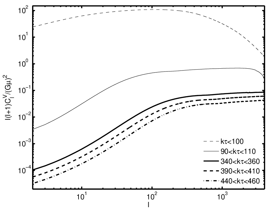
When our modified version of CMBEASY is applied to the eigenvalues and eigenvectors from the higher blocks, the temperature and polarization power spectra returned also have effectively the same form, except for the approximate re-scaling:

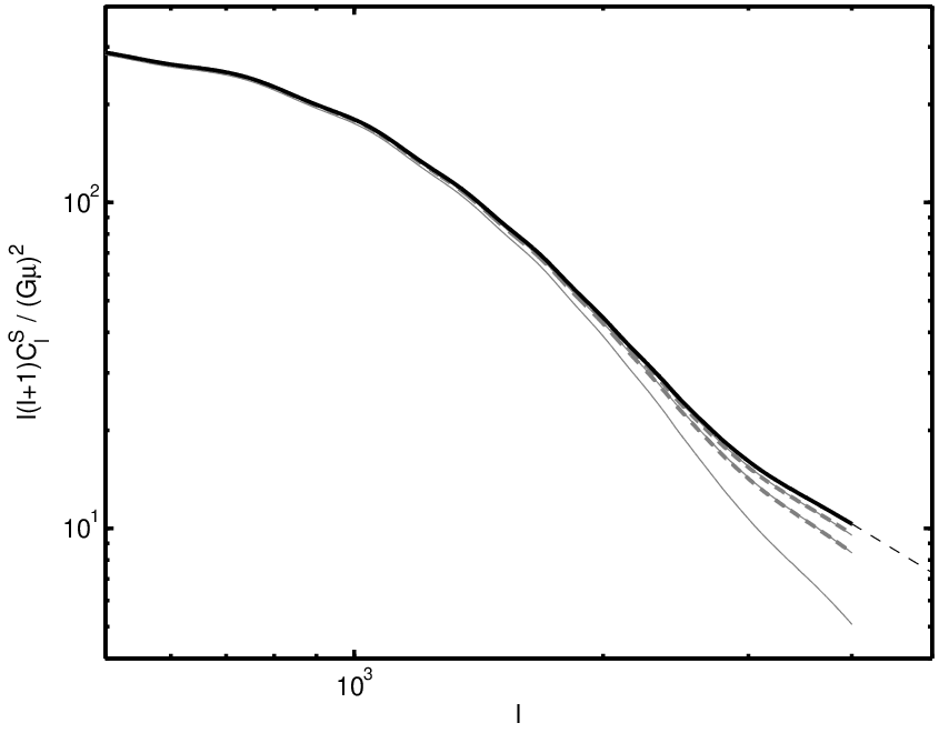
where $\kappa_{m}$ is the central $k\tau$ value of the $m$th block while $\beta\approx 2$ is a constant to be determined. This is illustrated for the vector mode in Fig. 10. It can also be seen that the contribution from a given block rises as approximately $\propto\ell$ up to a plateau for $\ell\approx\kappa_{m}\rightarrow 200\kappa_{m}$ before rapidly decaying for higher $\ell$. The key point is that given this scaling, we can find an approximation to the CMB power spectrum contribution from $k\tau$ values beyond the maximum value for which we perform full calculations $\kappa_{\mathrm{full}}$, by simply summing over many such re-scaled forms until the desired accuracy is reached. The total power spectrum is hence:

which is shown in Fig. 11 for the scalar mode. Furthermore, since $\mathcal{P}_{\ell}^{m}$ decays rapidly for $\ell\gtrsim 200\kappa_{m}$, then we may extrapolate the sum for $\ell\rightarrow\infty$ with $m_{\mathrm{max}}\rightarrow\infty$ by approximating it as an integral, which then varies as:

independent of the detailed form of the function $f(\ell)$. For $\beta\approx 2$, this yields roughly the $1/\ell$ form expected at very small angular scales due to the GKS effect [33], as will be discussed in Sec. IV.1.2. For the scalar, vector and tensor modes respectively we find $\beta=2.5$, $1.9$ and $1.7$ and we hence tentatively predict that the CMB contributions from each vary as $\ell^{-1.5}$, $\ell^{-0.9}$, $\ell^{-0.7}$ at very high $\ell$ (see next section).

Note that the use of this approximate re-scaling property is applied only to $k\tau$ values for which our knowledge of the UETC scaling functions is arrived at via power-law extrapolation. That is, we perform full CMB calculations for the range of $k\tau$ for which the simulations provide direct information, and it is fortunately the case that these provide the overwhelmingly dominant contribution for scales $\ell\lesssim 1500$, while in the present article we are limiting ourselves to $\ell\leq 4000$ and hence the extrapolations made are fairly reliable.

CMB polarization anisotropies differ from those for temperature in that they are created almost exclusively at recombination. Since the polarization is caused by Thompson scattering in the presence of a quadrupole anisotropy, the universe must be ionized in order to create it, but with Thompson scattering still weak enough for it not to have suppressed the quadrupole too heavily. Polarization is hence created only very close to recombination, and also weakly during the recent re-ionized epoch. As a result, the polarization signal comes primarily from horizon-scale UETC power impacting at times close to recombination. The contributions from high $k\tau$ near last scattering are outside our window of interest $\ell\leq 4000$ and are suppressed by Silk-damping. Further, the contributions from high $k\tau$ at recent times are negligible because there is little UETC power at such scales and the re-ionization contribution is secondary in importance. Our present results, shown in Fig. 16, therefore add little new information for CMB polarization from strings beyond our previous results [24, 22].

However, for completion, it should be noted that while the string contribution is sub-dominant for all scales in the E-mode polarization spectrum (EE) and the cross correlation of the E-mode with temperature spectrum (TE), it may dominate the B-mode polarization spectrum (BB) for scales $\ell\lesssim 400$. This is possible because the inflationary scalar mode contributes to BB only via weak gravitational lensing, which converts EE power into BB. Furthermore, our results indicate that the string contribution peaks at significantly lower $\ell$ than the weak lensing contribution, which should readily prevent confusion between the two, while the weak-lensing contaminant can also be partially removed [74]. Note that we find a BB peak from strings that is at larger scales than is seen in USM results when that model is set to approximate Nambu-Goto simulations [46], as expected given our lower string densities, and that the USM results suggest more confusion with the weak-lensing signal. It is also possible that the inflationary tensor mode may make a sizable contribution to the BB spectrum at very large angular scales, as shown in Fig. 16, but its normalization depends on the details of the inflationary model and is poorly constrained by current data. A wealth of B-mode data will soon be available and promises to be highly sensitive to cosmic strings [74, 24, 46].