Properties of the Top Quark
Abstract
The top quark was discoverd at the CDF and D0 experiments in 1995. As the partner of the bottom quark its properties within the Standard Model are fully defined. Only the mass is a free parameter. The measurement of the top quark mass and the verification of the expected properties have been an important topic of experimental top quark physics since. In this review the recent results on top quark properties obtained by the Tevatron experiments CDF and D0 are summarised. At the advent of the LHC special emphasis is given to the basic measurement methods and the dominating systematic uncertainties.
pacs
14.65.HaTop quarks1 Introduction
The aim of particle physics is the understanding of elementary particles and their interactions. The current theory of elementary particle physics, the Standard Model, contains twelve different types of fermions which (neglecting gravity) interact through the gauge bosons of three forces [1, 2, 3, 4]. In addition a scalar particle, the Higgs boson, is needed for theoretical consistency [5]. These few building blocks explain all experimental results found in the context of particle physics, so far.
Nevertheless, it is believed that the Standard Model is only an approximation to a more complete theory. First of all the fourth known force, gravity, has withstood all attempts to be included until now. Furthermore, the Standard Model describes several features of the elementary particles like the existence of three families of fermions or the quantisation of charges, but does not explain these properties from underlying principles. Finally, the lightness of the Higgs boson needed to explain the symmetry breaking is difficult to maintain in the presence of expected corrections from gravity at high scales. This is the so called hierarchy problem.
In addition astrophysical results indicate that the universe consists only to a very small fraction of matter described by the Standard Model. Large fractions of dark energy and dark matter are needed to describe the observations [6, 7, 8, 9, 10]. Both do not have any correspondence in the Standard Model. Also the very small asymmetry between matter and anti-matter that results in the observed universe built of matter (and not of anti-matter) cannot be explained until now.
It is thus an important task of experimental particle physics to test the predictions of the Standard Model to the best possible accuracy and to search for deviations pointing to necessary extensions or modifications of our current theoretical understanding.
The top quark was predicted to exist by the Standard Model as the partner of the bottom quark. It was first observed in 1995 by the Tevatron experiments CDF and DØ [11, 12] and was the last of the quarks to be discovered. As the partner of the bottom quark the top quark is expected to have quantum numbers identical to that of the other known up-type quarks. Only the mass is a free parameter. We now know that it is more than 30 times heavier than the next heaviest quark, the bottom quark.
Thus, within the Standard Model all production and decay properties are fully defined. Having the complete set of quarks further allows to verify constraints that the Standard Model puts on the sum of all quarks or particles. This alone is reason enough to experimentally study the top quark properties. The high value of the top quark mass and its closeness to the electroweak scale has inspired people to speculate that the top quark could have a special role in the electroweak symmetry breaking, see e.g. [13, 14]. Confirming the expected properties of the top quark experimentally establishes the top quark as we expect it to be. Any deviation from the expectations gives hints to new physics that may help to solve the outstanding questions.
Since the last review on top quark physics in this journal [15] the luminosity at the Tevatron has been increased by more than an order of magnitude. Now measurements of the top quark mass are no longer limited by statistical but by systematic uncertainties. Even discussions about the knowledge of the implicitly used theoretical mass definition become relevant. Moreover measurements of additional top quark properties now reach a viable precision. In this review the recent results on top quark properties obtained by the Tevatron experiments CDF and DØ are summarised. At the advent of the LHC special emphasis is given to the basic measurement methods and the dominating systematic uncertainties. Other reviews with different emphases are available in the literature [16, 17, 18, 19, 20, 21, 22, 23, 24].
After a short introduction to the Standard Model and the experimental environment in the remainder of this section, Chapter 2 describes the current status of top quark mass measurements. Then measurements of interaction properties are described in Chapter 3. Finally, Chapter 4 deals with analyses that consider hypothetical particles beyond the Standard Model in the observed events.
1.1 Theory
The physics of elementary particles is described by the Standard Model of particle physics. It describes three of the four known forces that act on elementary particles, the electromagnetic and the weak force are unified in the GSW-theory [1, 2, 3], the strong force is described by quantum chromodynamics (QCD) [4]. So far the influence of gravitation could not be unified with the other three forces in a consistent quantum theory. Due to its weakness it is usually safe to neglect its influence in the context of particle physics.
In the following a short description of the Standard Model shall be given to set the stage for later descriptions. For this the natural units where will be used.
1.1.1 The Standard Model
Lagrangian
The Standard Model is a quantum field theory with local gauge symmetry under the group . Its Lagrangian contains fields corresponding to three types of particles: Gauge or vector bosons, fermions and scalars. Gauge boson are described by vector fields, , scalars by complex fields, . Fermions can be described by Weyl spinors, , with left and right handed helicity. Using Einstein’s summation convention the Lagrangian can be written as
| (1) | |||||
Here capital Latin letters run over the gauge bosons, lower case Latin letters over the scalar fields and Greek letters , index the fermions of the standard model. and are Dirac indices. The field tensor is defined as
| (2) |
where are the structure constants of the gauge group. The covariant derivative is defined from the gauge symmetry to be
| (3) |
Here is the coupling strength for the gauge boson , i.e. , or . are the generators of the gauge symmetry in the representation that corresponds to the particle field on which the derivative acts.
| (4) |
where is the vector of Pauli matrices. The positive sign applies to fermions of right handed helicity, the negative for left handed ones.
The Yukawa couplings, , are free parameters that may be non-zero only when the combination of the fermions and with the scalars is gauge invariant. is a quartic form.
Particle Content
The particle content of the Standard Model is specified by defining the representations of the gauge symmetry for each of the fields contained.
The Weyl spinors describing the fermions transform according to fundamental representations for each of the subgroups or may be invariant under a subgroup. Quarks transform under the three dimensional representation of the group, . All left handed spinors transform under according to the two dimensional representation, , while the right handed spinors are singlets, i.e. invariant under rotations. This reflects the left handed nature of weak interactions. The transformation properties under are specified by the hypercharge. In the Standard Model all representations are repeated three times and build the three generation of fermions.
In Tab. 1 the representations of the fermions of the Standard Model are summarised. The representations of the non-Abelian gauge groups and are specified by their dimension (in bold-face), the hypercharge corresponding to the group is given as index.
| Gene- | Quarks | Leptons | |||
|---|---|---|---|---|---|
| ration | |||||
| 1st | |||||
| 2nd | |||||
| 3rd | |||||
| Symbol | Representation | Coupling strength |
|---|---|---|
| g | ||
For a few years it is known from the measurement of neutrino oscillations [25, 26, 27, 6] that also the neutrinos have mass and thus right handed neutrinos should be added to Tab. 1. The necessary extensions of the Standard Model are not unique and thus they are usually not considered part of the Standard Model. In the context of top quark physics neutrino oscillations do not play any role and can thus be ignored for the purpose of this review.
The gauge bosons of a quantum field theory need to transform according to the adjoint representation of their sub-group. Thus we get eight gauge bosons for the symmetry, the gluons, three for and one for the symmetry, c.f. Tab. 2. In addition to the bosons and fermions described the Standard Model contains a complex scalar doublet, the Higgs doublet , which transforms according to . It is needed for symmetry breaking.
Symmetry breaking: Higgs mechanism
In nature the symmetry of the Standard Model is broken. The symmetry breaking is implemented by the Higgs mechanism [5], which assumes that the scalar isospin doublet has a vacuum expectation value. This is achieved by proper choice of parameters in the most general potential, , for the scalar field in Eq. (1). According to the symmetry this can be chosen to exist in the lower component of the doublet:
| (5) |
By expanding the complex scalar field around the vacuum expectation value first four real scalar fields are specified. Three of these can behave like longitudinal components of the gauge bosons, . Usually the theory is thus written in terms of three massive vector bosons , , , a massless vector boson, the photon , and the fourth real scalar field, the Higgs boson :
| (6) |
Here is the gauge boson of the (hypercharge) symmetry and the Weinberg angle is defined by the ratio of coupling constants
| (7) |
After this rewriting the theory remains invariant. The symmetry now corresponds to the electrical charge. So the Standard Model parts are quantum chromodynamics (QCD) and quantum electrodynamics with their and symmetries, respectively.
The Higgs mechanism not only yields massive vector bosons, it is also responsible for the masses of the fermions. For the specified particle content, the Yukawa terms in Eq. (1) may be non-zero for left-handed quark or lepton doublets paired with the corresponding right-handed quark and lepton -singlets. For the first generation these terms are
| (8) |
Corresponding terms can be written not only for the other generations, but in general also for fermion pairs between different generations. Unitary rotations in the three dimensional space of generations are commonly used to redefine the lepton and quark fields such that Yukawa couplings occur only between particles of the same generation. This provides the mass eigenstates of the quark and lepton fields. These rotations cancel in most terms of the Lagrangian. The only observable remainder of this rotation is the Cabibbo-Kobayashi-Maskawa (CKM) matrix [28, 29, 6] which occurs in the coupling of the bosons to quarks:
| (9) |
At the same time this is the only process in the Standard Model that connects the different generations. Numerically this unitary matrix has diagonal entries close to unity and off-diagonal entries that are around between the first and second generation, around between the second and third generation and even smaller for the transition of the first to the third generation [6].
1.1.2 Perturbation Theory
Predictions of the Standard Model for high energy reactions are so far generally performed in perturbation theory. The reactions are described as one or more point-like interactions between otherwise free particles. The allowed reactions can be read off the Lagrangian and are usually represented by Feynman diagrams. For example the Yukawa term yields an interaction vertex of the strength with two fermions and the scalar field .
Each Feynman diagram serves simultaneously as a diagrammatic description of the reaction and as a short hand notation for the corresponding computation of the transition amplitude. The quantum mechanical amplitude of a given process that transforms a set of initial state particles to a set of final state particles is given by the sum of all possible diagrams with the corresponding initial and final state particles as external lines.
Diagrams with few interactions usually give the largest contributions and higher order corrections are suppressed by factors of the additional coupling strengths. Thus calculations are usually performed in a fixed order of the coupling constant(s). In some cases, however, kinematic enhancements of logarithmic type may compensate the suppression by additional powers of the coupling constant. Notably these occur in cases of collinear or soft gluon radiation and for top quark pair production near threshold. In these cases resummation of the leading (or next to leading) logarithms to all order of the coupling are performed.
Diagrams of higher orders generally involve loops which require to integrate over all possible momenta of the internal lines. Naively, such integrals diverge. It is necessary to renormalise the theory in order to obtain finite predictions. There are several possible schemes to perform this renormalisation. Most commonly the so called scheme is used, which itself depends on a continuous parameter the renormalisation scale . The dependence of results on the choice of this parameter is often used as a measure for theoretical uncertainties of a prediction.
Perturbation theory described so far deals with the particles of the Standard Model named above, i.e. with quarks, leptons, gauge bosons and the Higgs boson. In nature, however, quarks have not been observed as free particles, rather they are confined in bound states of colour neutral hadrons. The dynamics of quarks and gluons inside hadrons cannot be described by perturbation theory.
To describe the collisions of hadrons with perturbation theory the (soft) physics that governs the behaviour of quarks and gluons in the hadron needs to be factorised from the hard process in the collisions. The partons inside an incoming hadron are considered as a number of “free” partons that may enter the hard interaction. The distribution of partons inside the incoming hadron is taken from parton distribution functions (PDFs) that are derived from experiments. With this the cross-section, , to produce final state particles can be described in terms of cross-sections of incoming quarks and gluons to produce :
| (10) |
Here is the centre-of-mass energy squared of the incoming hadrons. At the Tevatron Run II . The colliding partons carry momentum fractions and , and is their centre-of-mass energy squared. and are the parton distribution functions for the partons and , i.e. the probabilities to find this parton in the proton and anti-proton, respectively. Formally, the parton density functions , and the partonic cross-section, , depend on the factorisation scale, , which specifies which effects are included in the PDFs and which remain to be described by the hard matrix element. They also depend on the renormalisation scale, . These dependencies are not written out in Eq. (10).
1.1.3 Top Quark Production in Hadron Collisions
††feynman-diagram: (Feynman diagram, (x2) ††feynman-diagram: (Feynman diagram, (x2) ††feynman-diagram: (Feynman diagram, (x2)
In hadron collisions, like the proton-antiproton collisions at the Tevatron, top quarks can be produced singly or in pairs. The pair production occurs dominantly via the strong interaction. In leading order the quark anti-quark annihilation and gluon fusion processes shown in Fig. 1 contribute. In higher orders also quark-gluon processes exist. The relative contribution of these diagrams depend on the parton distribution functions. At the Tevatron with a centre-of-mass energy of next-to-leading order predictions lead to an expectation of contribution from annihilation and from gluon fusion. The total cross-section of top quark pair production has been computed in perturbation theory using various approximations [30, 31, 32, 33, 34, 35]. Its value has a significant dependence on the top quark mass, which near the world average value is about . For a top quark (pole) mass of Moch and Uwer [34] find , based on the CTEQ6.6 [36] PDF. The uncertainty includes uncertainties of the PDF and the scale uncertainty.
Single top quark production can only take place via the weak interaction. The leading processes are quark annihilation through a boson, also called -channel, the quark gluon fusion with a boson in a -channel, c.f. Fig. 2, and production of single top quarks in association with a (close to) on-shell -boson. Charge conjugate diagrams apply for anti-top quark production. At the Tevatron Run II the cross-section to produce a single top or anti-top quark is . The - and -channel contribute a little less than and , respectively. The associated production contributes less than [37, 38, 39]. These numbers were derived assuming and using the MRST2004 [40] PDFs.
††feynman-diagram: (Feynman diagram, (x3) ††feynman-diagram: (Feynman diagram, (x3)
After production top quarks decay very rapidly through the weak interaction into a boson and a quark. In the Standard Model contributions from decays to light quarks are suppressed due to the smallness of the corresponding entries of the CKM matrix. The expected decay width of about corresponds to a lifetime of the order of [6]. Thus the top quark decays before it can couple to light quarks and form hadrons. The lifetime of bound states, toponium, is too small, , to allow for a proper definition of a bound state as already pointed out in the early 1980s [41].

The decay modes are defined purely by the boson decays. bosons may decay to quarks, i.e. hadronically, or leptonically. For top quark pairs this yields three basic decay modes: the all hadronic channel, the semileptonic channel and the dilepton channel. The all hadronic channel has a branching fraction of . Each of the three charged Standard Model leptons contributes in the semileptonic channel. The dileptonic decays have a total branching fraction of . See Fig. 3 for a graphical representation. Decays that involve leptons are usually not considered in analyses of the semileptonic and dileptonic decay modes, because leptons are difficult to identify. The analyses, however, include the events in which the tau decayed to an electron or muon.
Following this experimental nomenclature the semileptonic and dileptonic channels are considered to include only electrons and muons. If an analysis considers identified tau leptons this fact shall be explicitly stated. For single top quark analyses so far only the leptonic boson decays (to electrons and muons) are considered.
1.2 Experiments
Up to recently only one collider provides centre-of-mass energies sufficiently high to produce top quarks: the Tevatron at the Fermi National Accelerator Laboratory (FNAL) near Chicago, IL, USA. At the two collision points typical general purpose experiments of present collider physics are positioned, CDF and DØ. Each consists of a cylindrical part that covers particles produced at large angles to the beam and two end-caps that detect particles at smaller angles. Close to the beam tracking and vertex reconstruction components are placed, followed to the outside by calorimetry and muon detection systems. Some more details of the Tevatron and the two detectors shall be described below.
1.2.1 The Tevatron
The Tevatron collides beams of protons and antiprotons. The protons and antiprotons are produced and pre-accelerated in a series of smaller machines and then filled into the Tevatron to circulate in opposite directions. In a first phase of operation between 1992 and 1996 the beams were accelerated to . This phase is commonly called Run I. After an upgrade the Run II started in 2001. The upgrade enables the Tevatron to accelerate the beams to a final energy of to yield a centre-of-mass energy of . Also the peak luminosity was gradually improved and now reaches a factor of approximately 10 over the Run I performance [43, 44].
In Run I an integrated luminosity of about was delivered to both experiments. This was sufficient to discover the top quark in proton-antiproton collisions with a centre-of-mass energy of [11, 12]. With the increased centre-of-mass energy a increased cross-section was achieved for top quark pair production. At the time of writing an integrated luminosity of more than was delivered to both experiments. Preliminary results using up to have been made public by the experiments.
It is currently foreseen to continue running the Tevatron at least until the end of 2010 and an extension into 2011 is being discussed. The total integrated luminosity is expected to increase by about for each year of running. Thus until the end of the Tevatron program the total luminosity will more than double compared to what has been analysed so far [45].
1.2.2 The CDF Detector
The Collider Detector at Fermilab (CDF) [46, 47, 48] is one of two detectors recording collisions at the Tevatron. The vertexing and tracking components, the calorimetry and muon detection systems as used in the Run II measurements shall be described shortly in turn.
The tracking system of CDF is placed in a solenoidal magnetic field. The heart of the CDF tracking for Run II consists of three separate silicon detectors. The innermost (L00) consists of a single layer of single sided sensors at a radius of about . The upgraded silicon vertex detector (SVX II) consists of five cylindrical double-sided layers that along the beam axis reach to from the centre of the detector at radii between and [49, 50]. Finally the intermediate silicon layer (ISL) consists of double-sided sensors in one central layer at and in two layers at and for the forward regions [51]. The tracking system is completed by wire drift chambers with an outer radius of . Their length of allows to cover the central region of . The tracking systems provides full coverage and thus precise tracking for to measure the momentum of charged particles, to find the primary vertex of the collision as well as to find possible secondary vertices from long lived particles like quark hadrons.
Outside the tracking system a time of flight system (TOF) based on scintillator bars is positioned. This allows particle identification and is used in identifying hadrons [52]. The solenoid that provides the magnetic field for the tracking system is placed between the TOF and the calorimetry.

The central electromagnetic calorimeter is composed of alternating layers of lead and scintillator. It covers the pseudo-rapidity range of . To detect more forwardly produced particles layers of lead and proportional chambers are installed at pseudo-rapidities . The hadronic calorimeter uses lead as absorber material. The central region and the end cap wall use scintillator as active material. The forward regions also use gas proportional chambers. In total the calorimeter covers pseudo-rapidities of . The calorimeter allows energy measurements and identification of electrons, photons, jets and missing transverse momentum.
The calorimeter is surrounded by several systems of drift chambers to identify muons. The ‘central muon system’ is placed at a radius of . Behind an additional 3.3 interaction lengths of steel of the return joke the central muon upgrade system is located. Both systems cover pseudo-rapidities of . The third system, the central muon extension, extends this coverage at . So called barrel muon chambers extend the coverage for . Track segments in these components are used to identify muons.
CDF uses a three-level trigger system. The level 1 system has a pipeline for beam-crossings. After the level 1 trigger the event rate is approximately . At level 2 trigger processors analyse a substantial fraction of the event and further reduce the rate to . The 3rd level consists of a cluster of computers which perform an optimised event reconstruction. With this information the event rate is reduced to about . The events selected by level 3 are stored permanently to tape.
1.2.3 The DØ Detector
The DØ (Dzero) detector [53, 54] is the second of the two detectors recording collisions at the Tevatron. It has been significantly upgraded to adapt to the reduced bunch distance and increased luminosity of the Tevatron Run II. The upgraded DØ detector shall be shortly described here.
The tracking system at the centre of DØ has been fully replaced since Run I and now consists of a silicon micro-strip tracker (SMT) and a scintillating-fibre tracker within a solenoidal magnet. The SMT consists of a barrel with four layers of single and double sided silicon micro-strip detectors with a total length of about 70 cm. The barrel is separated into six subsections along the beam-pipe. Each subsection is capped with a disk of silicon detectors (F-disks). Three additional F-disks are placed on each side further outside of the barrel. Larger disks (H-disks) are placed at distances of and from the beam pipe. The SMT barrel provides excellent --information, the disks provide - as well as - measurements. During a shutdown period in 2006 the DØ silicon system was extended by adding an additional layer of sensors directly on top of the beam pipe. This Layer-0 significantly improves the ability of vertex reconstruction. DØ measurements are usually performed separately for data taken before and after the installation of Layer-0. The two run periods are commonly denoted as Run IIa and Run IIb. Outside the SMT the central fibre tracker (CFT) is placed. It consists of scintillating fibres mounted on eight concentric support cylinders at radial distances between and covering to about . At each distance one layer of fibres is oriented along the beam axis and a second is mounted with stereo angles of of .

To the outside of the CFT the solenoidal magnet is placed that produces a magnetic field for the tracking components. It is followed by the calorimetry that consists of a pre-shower detector that is placed in front of the cryostat and the sampling calorimeter based primarily on uranium/liquid-argon inside the cryostat. The end-caps that cover the forward regions have a similar structure, i.e. a pre-shower detector and a calorimeter cryostat. The calorimeters consists of three regions. The innermost is the electromagnetic calorimeter which uses thin () plates of depleted uranium as absorber material. It is followed by the fine hadronic calorimeter with thick plates of uranium-niobium. The outermost subsection, the coarse hadronic calorimeters, uses thick (about ) absorber plates of copper (in the central) and stainless steel (in the end-caps). The active medium in all three regions is liquid argon. Additionally, inter-cryostat-detectors (ICD) are mounted between the central and the forward cryostat to improve on the incomplete coverage of the calorimeters at .
The DØ muon systems outside the calorimeter consist of tree layers of drift chambers, one inside and two outside a toroidal magnetic field. The central muon chambers cover with proportional drift chambers and have a magnetic field of . The forward muon chambers use mini drift chambers and a toroidal field of . They extend the coverage to .
Also DØ uses a trigger system with three stages. The first level consists of a set of hardware trigger elements that provide a trigger accept rate of . In the second level hardware engines and embedded microprocessors provide information to a global processor that considers individual detector information as well as correlations. It reduces the rate by a factor of about . The third level consists of a farm of computers that reduces the rate to based on a limited event reconstruction. The accepted events are stored to tape for offline analysis.
1.3 Basic Event Selection
The selection of events in general, in particular the selection of top quark events, is based on the reconstruction of a number of different objects: The primary vertex of the collision, electrons, muons, jets and transverse missing energy. In addition, to reduce the background, often methods to identify jets from -quarks are applied. In the following these objects shall be shortly described in turn.
The reconstruction of the primary vertex is determined by assigning well measured tracks to a common origin in the interaction region. The primary vertex is constructed event-by-event and is used as reference for some of the following objects.
Electrons are reconstructed by a combination of tracking and calorimeter information. Quality cuts on the tracks typically include a threshold of the order of and the matching energy deposit in the calorimeters should be well contained in the electromagnetic subsection. In the absence of bremsstrahlung the energy deposit is expected to have a small radius in the - plane. Sophisticated algorithms take into account bremsstrahlung photons. Discriminating observables include the relative sizes of the energy deposit in the hadronic and the electromagnetic calorimeter. DØ uses a fixed ratio of the electromagnetic to the total energy [56] while CDF uses an energy dependent cut on [57].
Muons are identified by the presence of signals in the dedicated muon chambers that can be matched to a track found in the tracking system. For this purpose CDF and DØ extrapolate isolated tracks with standardised quality cuts through the calorimeter out to the muon chambers to find matching track segments.
For both lepton objects different quality classes are defined, named “loose”, “medium”, “tight”, etc, with increasingly stricter requirements on the isolation of the track and the calorimeter cluster. These different criteria can be used to obtain an acceptable signal to background ratio. The selection of “loose” leptons excluding those that also have a “tighter” identification is often used to define sideband samples to extract background estimates from data. The triggering and reconstruction efficiencies are usually studied in events using the tag and probe method.
Jets are reconstructed from all calorimeter towers. They usually show a substantial contribution from the hadronic subsection and are usually broader than signals from electromagnetic particles. At the Tevatron experiments the “improved legacy” cone algorithms [58] with radii of and are used by CDF and DØ, respectively. Quality cuts typically require that the energy of a jet is not contained to more than in a single tower and deposits from electron and photon candidates are removed. The jet energy reconstructed from the calorimeter cells needs to be corrected for a number of effects. These corrections include imperfections of the calorimeter but also energy offsets due to contributions from the underlying event, multiple hadron interactions and noise in the electronics. This correction, usually called the Jet Energy Scale (JES), is obtained from precisely measured electromagnetic objects by assuming momentum conservation in the transverse plane for jets events.
Jets stemming from -quarks can be identified due to the long lifetime of about of the hadrons in such jets. At the typical energies in top quark events of to the mean decay length is of the order of . This fact is exploited by computing the impact parameter for tracks or by explicitly reconstructing a secondary vertex from the tracks that is displaced from the primary vertex. To identify -jets CDF uses only tracks that fall within the cone radius of the considered jet. A secondary vertex is reconstructed in two passes with different track requirements [59]. The 2d decay length is computed as the distance of primary to the secondary vertex. The significance, i.e. the decay length over its uncertainty, is required to be larger than 3. If the direction from the primary to the secondary vertex is opposite to the direction of the jet, the tag is called a negative tag. These negative tags are useful to determine the purity of mis-tag rates. In DØ first track jets are built with a cone algorithm independent of the calorimeter jets described above. Secondary vertices are reconstructed with tracks from a given track jet. Calorimeter jets are considered as identified -jets, if an identified track jet falls within a radius of . The most recent DØ tagging algorithm uses the impact parameters of tracks matched to a given jet and information on the secondary vertex mass, the significance of displacement, and the number of participating tracks for any reconstructed secondary vertex within the cone of the given jet. The information is combined in a neural network to obtain the output variable, , which tends towards one for -jets and towards zero for light jets [60].
The presence of a neutrino is inferred from the momentum imbalance in the transverse plane, that occurs because neutrinos are invisible to the detectors. If all objects of an event were measured the sum of the transverse momenta should vanish. Thus the sum of the transverse momenta of all neutrinos can be deduced from the missing transverse momentum needed to assure momentum conservation. It is derived from the calorimetric measurements and their direction with respect to the interaction region as the negative vector sum of the transverse energies and thus usually named Missing Transverse Energy, . The sum is taken over all calorimeter cells that remain after noise suppression. In general corrections for identified objects with known energies like electrons, muons or jets are applied.
Triggering and preselection of single top quark events and of top quark pair events in the semileptonic and dileptonic channels are based on reconstructed lepton, jet and objects described above. Typically the leptons and the missing transverse energy are required to have . Signal selection in addition requires the presence of jets also with a typical momentum requirement . The number of jets required of course depends on the channel under consideration. Some analyses here improve the signal to background ratio by requiring one or more identified -jets. Others construct a likelihood for an event being top quark like based on topological quantities to consciously avoid -jet identification. Additional cuts may be introduced to enhance the signal to background ratio or to improve the data to Monte Carlo agreement. In the semileptonic selection DØ e.g. recently requires the leading jet to fulfil and avoids events in which missing transverse momentum and the selected lepton are aligned.
Events of the all-hadronic channel have to be selected by requiring multijet final states. Due to the overwhelming background from multijet events in these analyses usually stronger cuts are applied on the transverse momentum of the jets.
2 Top Quark Mass Measurements
The mass is the only property of the top quark that is not fixed within the Standard Model of particle physics. The Yukawa coupling responsible for the coupling of the top quark to the Higgs boson and thus for the mass of the top quark is a free parameter of the Standard Model. This already illustrates the importance of measuring the top quark mass.
Moreover Standard Model predictions of electroweak precision observables depend on the value of the top quark mass via radiative corrections. By correlating the boson mass with the top quark mass the mass range for the yet undiscovered Higgs boson can be constrained. Measurements of the top quark mass are thus an important preparation for discovering the Higgs boson and will serve as a consistency check of the Standard Model after its discovery.
In the following theoretical aspects of fermion mass measurements are discussed, before the experimental methods used in the various decay channels are explained. Then issues of modelling non-perturbative effects in collisions and their influence on the existing measurements are discussed and the combination of the various measurements to a final result is reviewed. The conclusions contain a critical comparison of current results with expectations and future prospects.
2.1 Theoretical Aspects
For free particles the physical mass is usually taken to correspond to the pole of their propagator, i.e. their value of the four-momentum squared, . Because of confinement quarks cannot exist as free particles and this definition becomes ambiguous.
The definition of the pole mass is still possible on an order by order basis in perturbation theory, but is considered to be intrinsically ambiguous on the order of the confinement scale [61]. Mass definitions can also be obtained following other renormalisation schemes such as the -mass in the -scheme. Other definitions have been suggested by [62, 63].
The relation between the various mass definitions can usually be computed in perturbation theory. For the top quark the numerical values of the different definitions may differ significantly. In NNLO for example the -mass of the top quark is about smaller than the pole mass.
This large difference makes it important to understand which definition and order of perturbation theory of the top quark mass is measured by the experiments. As we shall see below, all direct methods to determine the top quark mass use Monte Carlo simulation to either extract the mass or calibrate the procedure. Thus the question really is, which definition of the top quark mass is used as a parameter in these Monte Carlo generators.
Unfortunately, it is not well understood which field theoretic mass definition the currently used generators correspond to. Clearly, as the hard matrix elements of (most) generators is implemented in leading order, they correspondingly use the leading order mass. It is usually argued that this corresponds to the pole mass, because in the pole mass definition any shifts of the position are to be absorbed in the mass definition. Monte Carlo generators do not absorb corrections from the parton shower or the hadronisation into the mass definition. And it is not clear in how far the parton shower and the modelling of hadronisation alter the mass definition, nor which approximation of QCD this mass parameter corresponds to. Partial answers have been given in [63], but at this point a conceptual uncertainty remains that is considered to be of the order of .
Comparisons of the top quark mass from direct measurements with electroweak precision data to determine e.g. the Higgs boson mass currently assume the measured top quark mass values corresponds to the pole mass definition. They thus have to be interpreted with care.
Experimentally precise measurements of the top quark mass are nevertheless useful. On the one hand they are needed to set the mass parameter for simulating top quark events, which will be important backgrounds for some LHC searches. On the other hand the consistency between the various experimental methods and the top quark decay channels gives confidence in these methods. Finally, it seems feasible that a theoretically more precise specification of the top quark mass definition used in the Monte Carlo generators can be derived in the future [64]. Any bias from the interpretation as a pole mass may then be corrected for.
2.2 Lepton plus Jets Channel
The lepton plus jets channel is considered to be the golden channel in top quark mass measurements. Due to a lepton and a neutrino in the final state it has a good signal to background ratio. In addition one of the top quark quarks is fully measured in the detector.
Several method have been applied by CDF and DØ to measure the top quark mass in this channel. The methods exploit the kinematics of the events to different levels and make different assumptions about details of the production mechanisms.
2.2.1 Template Method
The basic template method was already applied to lepton plus jets events in the papers describing the first evidence and discovery of the top quark.
In this method a top quark mass is reconstructed for the each of the selected events using the momenta measured for lepton and jets and the transverse missing energy. The distribution of the reconstructed masses is then compared to template distributions from simulation. These templates are constructed from signal Monte Carlo with varying top quark mass values and contain the expected amount of background events. The method thus relies on good Monte Carlo modelling of signal and background.
CDF Run II Template Measurement
CDF has applied an improved template method in up to of data combining the lepton plus jets channel and the dilepton channel [65, 66, 67, 68]. For clarity the two analysis parts will be described separately. The dilepton portion of this analysis can be found in Section 2.3.1.
Lepton plus jets events are selected requiring a single high lepton, large missing transverse momentum and at least four jets. Events are separated by the number of jets identified as -jets based on the transverse decay length of track inside the jet [69]. In case of only a single identified jet only events with exactly four jets are considered. For events with more than one identified -jet more than four jets are allowed.


In each event a top quark mass is fitted using a constrained fit. Besides the top quark mass, the momenta of the top quark decay products (the quarks and leptons) are fitted to the observed transverse jet and lepton momenta, , and the unclustered energy, . The unclustered energy is the calorimetric energy in the transverse direction not associated with any reconstructed object. Jet momenta are corrected to parton level with CDFs common jet energy scale correction. The invariant masses of the boson decay products on both sides, and , are constrained to be consistent with the nominal boson mass within the boson width. The reconstructed top quark mass is required to be consistent within the top quark width with the invariant mass of the top quark decay products on both sides, and . The fit thus is written as
| (11) | |||||
The fitted unclustered energy, , is related to the transverse momentum of the neutrino used in the computation of and . This is computed for all possible associations of quarks to four jets, allowing -jets only to be matched with quarks. Only the top quark mass value of the association with the best fit is kept. If this best the event is rejected.
To constrain the jet energy scale simultaneously with the top quark mass, the dijet mass, , is measured from the non--tagged jets among the four leading jets without applying the above kinematic fit. This is only unique for events with two identified jets. In other events the two jets that yield the dijet mass closest to the -boson mass are chosen.
Thus for each event one top quark mass value, , and one dijet mass, , is entering the following analysis.
Monte Carlo simulations are used to determine the expected behaviour of signal events as well as the background contributions. The dominant jets background is simulated with Alpgen+Pythia [70, 71] with a normalisation derived from data. The multijet background is modelled with samples containing non-isolated leptons. Smaller background from single-top and diboson events are taken from Monte Carlo with normalisation to theoretical cross-sections. All backgrounds are assumed to have no dependence on the nominal top quark mass, but are allowed to vary with the jet energy scale. Signal samples for various nominal top quark mass values, , are generated using Pythia. All simulations are passed through the full CDF detector simulation and reconstruction.
These simulations are used to generate probability density functions, , to find a signal event with measured values and given a nominal top quark mass, and jet energy scale shift, . Similarly a probability density for background events, , is computed as function of the jet energy scale shift, only. CDF uses a Kernel Density Approach, where each simulated event contributes not only with its reconstructed values and , but also in the neighbourhood around these. The size of this neighbourhood is controlled by smoothing parameters. The parameters are chosen dynamically: small near the maximum of a given distribution where the statistics require less smoothing and larger in the tails. Examples of the resulting density functions are shown in Fig. 6.
With these probability densities the likelihood is constructed. The number of signal and background events in the single -tag and the double -tag sample are used as additional parameters with Gaussian constraints on the background estimations obtained above. Also the jet energy shift, , is constrained by a Gaussian term to be consistent with zero within its nominal uncertainty, .
| (12) |
Here indicates the subsamples with one or more than one identified -jets, respectively. and are the number of signal and background events and the background expectations in the samples.
The described likelihood formulae can only be evaluated at the discrete values of and for which simulations were run. To obtain the likelihood for arbitrary values of and a quadratic interpolation is used. The central result is obtained by maximising the likelihood and its uncertainty is quoted as the (largest) mass shift corresponding to a likelihood change of .
Systematic uncertainties are evaluated by modifying several aspects of the analysis described. The dominating uncertainty in top quark mass measurements is the jet energy scale. Through the simultaneous fit its contribution is part of the statistical uncertainty in this measurement. Residual effects remain through uncertainties in the and dependence. The uncertainty of modelling the top quark pair signal events is evaluated by comparing pseudo experiments generated with Pythia and Herwig. These two systematic uncertainties contribute with about to the uncertainty and are the two largest single contributions to the systematic uncertainty. Additional contributions in order of decreasing importance include the uncertainties on modelling colour reconnection [72, 73, 74], the background shape, the parton density functions.

With of data using the lepton plus jets channel only CDF determines a top quark mass of [68]
| (13) |
For the jet energy scale shift the fit yields , very consistent with the external jet energy scale but with a significantly reduced uncertainty. Combining the results with an analogous measurement in the dilepton channel which uses a consistent jet energy scale shift (c.f. Section 2.3.1) yields
| (14) |
The likelihood contour of the two dimensional measurement of and is shown in Fig. 7.
DØ Run II Template Measurements
DØ has produced preliminary results for top quark mass measurements using the template method [75, 76]. The method differs from the CDF method as the templates are not smoothened and in the use of a binned likelihood. As these results were not updated nor published in the last years they shall not be described in more detail here.
2.2.2 Ideogram Method
The ideogram method was transfered to top quark mass measurements from a method used in the DELPHI boson mass measurement [77, 78].
Also this method relies on an event by event reconstruction of top quark mass values. But in contrast to the template method the signal likelihood is constructed event by event from the theoretically expected Breit-Wigner distribution smeared with the experimental resolution of each individual event. Events with a configuration that allows a more precise reconstruction thus contribute more than events with a configuration that is difficult to reconstruct.
DØ
DØ has published an analysis of of data based on semileptonic top quark pair events [79]. The event selection requires an isolated lepton, missing transverse energy and four or more jets. To identify quark jets the decay length significance of a secondary vertex reconstruction is used [80]. No cut is placed on the number of identified -jets.
The top quark mass in each event is reconstructed using a constrained fit that determines the momenta of the top quark pair decay products ( from the measured momenta of the charged lepton, the four leading jets and the missing transverse momentum and their uncertainties. Constraints are placed on the invariant mass of the two light quarks and the two leptons, respectively, which are required to be consistent with the boson mass. The reconstructed top and anti-top quark masses are required to be equal. The 12 possible assignments of jets to quarks that yield different constraints are considered. In addition two possible solutions for the neutrino momentum are considered, which results in 24 top quark mass values per event. As the common jet energy scale of DØ corresponds to the particle level, i.e. what would be visible in an ideal detector, the fit uses jet-parton mapping functions determined from Pythia simulation. These mappings contain an overall scale factor, , for the jet energy scale that may modify the default jet energy scale.


The described fit is repeated for various values of the jet energy scale factor, so that the resulting mass values and the fit are functions of . Through the constraints to the nominal boson mass, the fit is expected to be the smallest for the correct jet energy scale (and top quark mass value). Events with no jet-parton combination reaching at the central jet energy scale are rejected at this point.
To determine the expected performance of the selection and the corresponding background contamination, top quark pair signal for various nominal top quark mass values and jets background events are generated using Alpgen+Pythia. The events are passed through the full detector simulation and reconstruction. Multijet background is modelled with side band data obtained from inverted lepton quality cuts. The sample composition is determined from a likelihood discriminant that combines topological observables, with tracking based jet shape and tagging information, c.f. Fig. 8. The observables are selected to have low correlation to the top quark mass.
An event by event likelihood is now constructed to observe the top quark masses reconstructed in the kinematic fit, the discriminant and the number of identified -jets given the nominal values of and :
| (15) | |||||
Here represents the measured observables for the event under consideration and is the signal fraction of the corresponding sample. The signal and background probabilities, and , are proportional to the probabilities to find signal or background at the observed discriminant value. Because of the selection of observables in the discriminant, this factor does not depend on the top quark mass and the jet energy scale and is factorised as:
| (16) |
The top quark mass and jet energy scale dependent portion of the signal probability, , is computed as the sum over all 24 jet-parton assignments and neutrino solutions. Their relative weight, , is computed from the probability of the kinematic fit and in presence of identified -jets includes the probability for the quarks associated to the -jets to produce a tagged jet. Because the result of the kinematic fit depends on the jet energy scale factor the weights depend on .
| (17) |
The background probabilities are obtained from the simulated jets events. The signal probabilities are computed as the convolution of a Breit-Wigner, , that describes the theoretical distribution of mass values and a Gaussian, , that represents the detector resolution. As this ansatz is valid only for the correct jet-parton assignment and because the wrong pairings do contain information about the top quark mass, a second contribution to describe wrong pairings is added:
| (18) |
with being the fraction of events in which the weight is assigned to the correct jet-parton pairing. For the width of the Gaussian the uncertainty, , of the mass determination obtained in the constrained kinematic fit is used. Thus events with a well-determined mass from the kinematic fit contribute more than events with a less precise fit result. The expected mass value distribution in wrong pairings, , also contains information about the true top quark mass. It is determined from simulation as function of the number of identified -jets. Also the background function, , is taken from simulation.
Due to the presence of wrong jet-parton assignments and background events the described likelihood does not yield unbiased results for the jet energy scale factor, . The likelihood is thus corrected with an -dependent but mass-independent correction factor.

The likelihood for the complete sample of observed events is then simply the product of the jet energy scale corrected likelihood, , for all individual events:
| (19) |
This likelihood is maximised simultaneously with respect to the top quark mass, , the jet energy scale factor, and the signal fraction .
Before this procedure is applied to data its performance is determined on large numbers of pseudo experiments with varying nominal parameter values. The bias is determined as the mean difference between the nominal value and the measured result. The correctness of the fit uncertainty is checked from the distribution of pull values, i.e. the distribution of differences between the measured values and their means normalised to the individual fit error. The bias and the width of the pull distributions for the fitted top quark mass and jet energy scale factor, , are determined as function of the nominal top quark mass and jet energy scale factor simultaneously. Linear corrections are applied to correct for the obtained biases and to correct the uncertainty for any deviation of the pull width from the ideal value of one.
Systematic uncertainties for this measurement are determined from pseudo experiments with events shifted according to the systematic variation under study. Due to the two dimensional fit the uncertainty of the overall jet energy scale is contained in the uncertainty obtained from the likelihood fit. Residual discrepancies between the data and Monte Carlo energy scales still affect the result and give the largest contributions to the systematic uncertainties. DØ evaluates uncertainties due to quark fragmentation modelling [81] and the calorimeter response to -jets to and , respectively. The uncertainty from the of the jet energy scale yields . Another large contribution of comes from the signal modelling which is estimated by varying the fraction of high energy gluons produced in addition to a top quark pair. Further uncertainties include the influence of uncertainties on the trigger efficiencies, the background modelling and the calibration.
The ideogram method with in-situ jet energy scale calibration applied in of data [79] yields a top quark mass of
| (20) |
the jet energy scale factor is determined to be consistent with the nominal value of , which corresponds to the calibration obtained in jet-photon events. The fit probability contour lines for the individual lepton channels and the combined results are shown in Fig. 9.
2.2.3 Matrix Element Method
The Matrix Element method in the lepton plus jets channel was pioneered by DØ in Run I [82] and is based on ideas described in [83, 84]. In this method the likelihood is constructed according to the expected distribution from the mass dependent top quark pair production matrix element. With respect to the previously described methods this includes additional information from top quark mass dependent kinematics into the measurement.
DØ
Results for the top quark mass using the Matrix Element method have been regularly updated with DØ Run II data [85, 86, 87, 88] with the latest result including of data. The analyses select events from semileptonic top quark pair decays by requiring a single isolated lepton, missing transverse momentum and exactly four jets. In the recent analyses at least one of the jets needs to be identified using DØ’s neural network jet identification [60]. Vetoes are applied on additional leptons and on events in which the lepton and the missing transverse momentum are close in the azimuthal direction.
The top quark mass and an overall jet energy scale factor are determined simultaneously from an event by event probability that the observed event may occur given the assumed values of the top quark mass, , the jet energy scale factor, and the signal fraction :
| (21) | |||
Here represents the measured momenta of the lepton, the jets and the missing transverse momentum. is the probability for the configuration to be accepted in the analysis. The probabilities, and , for signal and background events to be observed in the configuration given the set of parameters, , and , are computed from matrix elements of the dominating processes.


The signal probability is computed from the matrix element for top quark pair production and decay through quark anti-quark annihilation , convoluted with the transfer function, , that describes the probability to observe a parton configuration, , as the measured quantities, .
| (22) | |||
The sum is over the possible flavours of the incoming quarks and the integral over their momentum fractions, and , as well as the 6-body phase space for the outgoing particles, . are the parton densities for the incoming quarks and is the centre-of-mass energy squared. The normalisation factor is the cross-section observable with the selection used, i.e. it includes effects of efficiencies and geometric acceptance.
For the background probability a corresponding formula is used with the top quark pair matrix element replaced by the jets matrix element, which of course is independent of . The contribution from multijet events is considered to have a similar shape and is not included separately.
Both, and contain the same transfer function, . It is derived from full simulation for individual jets and leptons. Only changes of the size of the momenta but not of the directions are considered. Because it is not known which jet stems from which parton, a weighted sum over all 24 possible assignments is made. The weight, , reflects the probability of the event’s -tags to be consistent with the jet-parton assignment under consideration:
| (23) |
The values and are the measured and the assumed momenta of the lepton, is the measured momentum of the th jet and the momentum of the matrix element parton associated to the th jet in the jet parton association number . and are the transfer functions for leptons and jets, respectively, which are zero when the directions do not coincide.
The likelihood to observe the measured data is computed as the product of the individual event probabilities, :
| (24) |
For each assumed pair of the nominal top quark mass and the jet energy scale factor, and , the likelihood is maximised with respect to the top quark fraction, . In [85, 86, 87] the top quark mass and jet energy scale factor are then determined by maximising the two dimensional likelihood . In [88] the jet energy scale factor is constrained with a Gaussian probability distribution to its nominal value and its uncertainty as obtained from photon plus jet and dijet events.
Before the method is applied to data, its performance is calibrated in pseudo experiments. Random events are drawn from a large pool of simulated top quark pair signal and jets background events with proper fluctuations of the signal and background contribution such that the total number of events corresponds to the number of events observed in data. The simulated events were generated with Alpgen+Pythia and passed through the full DØ simulation and reconstruction. This procedure is repeated 1000 times for several fixed nominal values of , and . Thus for each of the nominal values the signal fraction, the top quark mass and the jet energy factor can be measured with the described procedure 1000 times. The mean result for each set of pseudo experiments with fixed nominal , and are compared to the nominal values in the calibration curves in Fig. 10. The final result is corrected for any deviation of these calibration curves from the ideal diagonal. Also the pull width is computed and the statistical uncertainty corrected accordingly.
The leading source of systematic uncertainty contributing (Run IIb) stems from the modelling of differences in the detector response between light quark and quark jets. The next important contribution arises from uncertainties modelling hadronisation and underlying event. It is estimated from the difference between Pythia and Herwig and contributes with nearly . Also the sample dependence of jet energy scale corrections in simulation contributes with this size. For the first time in [88] this measurement includes an estimate of the uncertainty due to colour reconnection effects [72, 73, 74], which contributes to the uncertainty. The squared sum of the individual contributions yields a total uncertainty of (Run IIb). DØ has applied this analysis to their dataset separated by run periods. The Run IIa result and the Run IIb result, shown in Fig. 11, are combined with the BLUE method [89] following the error categories used by the Tevatron Electroweak Working Group [90] (see also subsection 2.7 below) and yield
| (25) |
where in this combined result the uncertainty due to the overall jet energy scale factor is contained in the systematic uncertainty. This measurement is currently DØ’s most precise top quark mass result.

CDF
The CDF collaboration is using the concept to measure the top quark mass from a likelihood based on the production matrix element in the lepton plus channel in several variations [91, 92, 93, 94, 95, 96].
The recent analyses all base on an event selection that requires a single isolated lepton, missing transverse momentum and exactly four jets, at least one of which is required to be identified as jet. Then the top quark mass and an overall jet energy scale factor are determined simultaneously from an event by event probability that the observed event may occur given the true values of the top quark mass, , the jet energy scale factor, and the signal fraction . The various CDF analyses differ in the construction of the likelihood.
The CDF Matrix Element method (MEM) [91, 92] follows closely the procedure outlined in Section 2.2.3. The matrix element used to describe signal is that of the process with its decay. For background the jets matrix element is employed. Finally, the transfer functions of Eq. (23) use only parton-jet assignments consistent with -tagging information and assumes the lepton measurement to be exact. For the background probability, , the dependence on the jet energy scale is taken from a parameterisation of the average likelihood response rather than an explicit change of the transfer functions.
The Dynamical Likelihood method (DLM) [93, 94] differs from the Matrix Element method in that it bases its likelihood only on the signal contribution, . In this signal term the squared matrix element is factorised into a production matrix element, the (anti-)top quark propagators and their decay matrix elements: , which removes spin-correlations. However, in contrast to previously described measurements it includes gluon diagrams, i.e. can be or . For the treatment of background contributions the method fully relies on results obtained in ensembles of pseudo-datasets similar to the calibration step of the other methods. This correction is computed depending on the jet energy scale correction and the background fraction.
The Matrix Element Method with Quasi-MC-Integration (MTM) [97, 98, 99] uses an again more complete matrix element to construct the signal likelihood. The applied matrix element [100] includes the and the production channels with full spin-correlations. The method treats the background by subtracting the expected contribution of the logarithm of the likelihood. Equation (21) is thus rewritten as
| (26) |
with being the average obtained in background events. The expected background fraction, , is computed from simulation and applied event by event as function of the output of a neural network discriminant, c.f Fig. 12.

Moreover the analysis removes events which are likely to be mismeasured, e.g. due to extra jets, misidentification etc. For this events are required to have for at least some range of .


In all methods the overall likelihood is computed from the various event likelihoods following Eq. (24). It is maximised to find the optimal top quark mass and jet energy scale parameters. For the MEM also the background fraction is fitted. The performance is then checked by applying the top quark mass measurement on ensembles of pseudo-experiments with various nominal values of the top quark mass, , and the jet energy scale shifts, . The results are corrected for any observed shifts and the uncertainties scaled to fit the observed spread of results in the ensemble tests. The observed shifts vary between for the Dynamical Likelihood method [93], which relies on this calibration to describe the background effects, and for the Matrix Element method [92], which has the most complete background term.
As all methods apply an in-situ jet energy calibration this important systematic is already covered by the uncertainty of the fit result. The residual effect of the jet energy scale is estimated by varying the and dependence. The uncertainty of the jet energy scale of -jets from various sources is considered separately. The uncertainty of signal modelling is determined from comparison of Pythia and Herwig and by varying the amount of initial and final state radiation produced in the parton shower. Further uncertainties include an estimate of the background modelling and treatment in each method. The DLM has the uncertainty due to initial and final state radiation as the most important single contribution, while in the MEM and the MTM the residual jet energy scale and the difference between generators used for signal simulation are the two leading contributions. In MEM and MTM colour reconnection effects [72, 73, 74] are estimated and yield significant contributions of and , respectively.
The most recent results of the various Matrix Element like methods of CDF were obtained at different integrated luminosities. All results yield in-situ jet energy scale corrections consistent with the default calibration used in CDF.
| (27) |
where the first uncertainty is the statistical one and includes the overall jet energy scale uncertainty, the second uncertainty is the systematic one. The two dimensional representation of these results which simultaneously determine the jet energy scale are shown in Fig. 13. These measurements of course use (partially) the same data, thus for the combination only the most precise one is used, until their correlation is determined.
2.2.4 Decay Length and Lepton Momentum Methods
The top quark mass measurements described so far, aimed to use the maximal available information to yield the best statistical uncertainty for the given number of events. However, all these measurements have significant uncertainties from the jet energy scale. Alternative observables that have little or no dependence on the jet energy scale are therefore an interesting complement.
In the lepton plus jets channel of top quark pair decays CDF has investigated two observables: the transverse decay length of tagged jets and the lepton transverse momentum. One analysis combines the mean values of both observables [101, 102] while the other uses the mean and distribution of the lepton transverse momentum alone [103].
Two observable mean value method
For the method using both observables the data selection requires one isolated lepton, missing transverse momentum and at least three jets. For events with exactly three jets two of the jets need to be identified as jets with CDFs secondary vertex algorithm [69]. For events with four or more jets only one needs to have such a reconstructed secondary vertex.
The expected sample composition is determined from a combination of data and simulation. Top quark pair signal is simulated using Pythia with CTEQ5L parton densities for various nominal top quark mass values. Also single top quark samples are generated with various nominal top quark mass values. The dominating background jets is simulated with Alpgen+Pythia, the multijet background is modelled from a data sample with modified lepton selection criterion. All simulated events are passed through the full CDF detector simulation and reconstruction.


For the top quark mass determination the transverse decay length of the tagged jets is measured with the vertex algorithm used for the selection above. The actual measurement is performed using the means of the observed decay lengths, , and the transverse lepton momentum, . The expected contribution from background is taken from the described background model. Because the observables chosen are sensitive to the details of the event kinematics the signal simulation is corrected to yield parton distributions consistent with CTEQ6M [36]. In addition the total contribution from gluon fusion is corrected as function of the top quark mass. The performance of the simulation for determining the decay length of the tagged jets is calibrated in a dijet control sample.
With these corrections the expected means of decay lengths and transverse lepton momentum and their expected statistical spread are determined as function of the nominal top quark mass using ensembles of pseudo-data. The curves obtained are fitted by quadratic polynomials to obtain smooth curves. Figure 14 (left, middle) shows the mean values and and the resulting top quark mass ranges from the individual observables. The combined result is obtained from the likelihood to find the observed mean values at various nominal top quark masses, c.f. Fig. 14 (right).
The dominant systematic uncertainties for the measurement from arises from the uncertainty on the modelling of initial and final state radiation in the signal simulation, from the lepton momentum scale and the shape of the background description. In the measurement from the uncertainty of the data to Monte Carlo correction for the decay length dominates the uncertainties. The jet energy scale gives a non-negligible contribution to the measurement from the average decay length through effects on the event selection.
In of data CDF measures the top quark mass from the mean decay length, , and the mean lepton momentum, to be [102]
| (28) |
where the jet energy scale uncertainty is included (as a small) contribution to the systematic uncertainty. The larger statistical uncertainty (compared to the Matrix Element methods) prevents a significant weight to the current combination of top quark masses [90].
Lepton momentum shape method
The analysis that concentrates on the transverse lepton momentum alone [103] is based on events with a single isolated lepton, missing transverse energy and at least four jets. At least one of the jets is required to be identified as -jet.
Top quark pair signal events are simulated for various assumed top quark mass values. Backgrounds due to jets, jets diboson and single top quark production are described with simulation. Estimates for multijet background with fake leptons and the normalisation for light flavour jets are derived from data. These signal and background models are used to determine parametrised templates for the distribution of the lepton spectrum as function of the top quark mass. To extract the top quark mass these templates are compared to the observed data using an unbinned maximum likelihood fit. Leptonic boson decays are used to calibrate the lepton .
The uncertainty of the final result is dominated by the statistical uncertainty. The systematic uncertainties are dominated by effects related to signal and background modelling. The uncertainty on the fake lepton description contributes with ; differences between generators for the signal modelling contribute with to the systematic uncertainty.
In of CDF data the top quark mass determined from the shape of the lepton momentum distribution is [103]
| (29) |
This result has been combined with a corresponding study of dilepton events [104], c.f. section 2.3.3, to yield [105]
| (30) |
The large statistical uncertainty of these methods prevents a significant contribution to the world average from such measurements at the Tevatron. Its independent and low systematics will make them more relevant at the LHC.
2.3 Dilepton Channel
Due to the small branching fraction the dilepton channel has much fewer events, but the two charged leptons also yield a much cleaner signature. For a measurement of the top quark mass the dilepton channel has the additional complication that the kinematics are under-constrained due to the two unmeasured neutrinos. Two of the six missing numbers can be recovered from the transverse momentum balance, two more from requiring that the invariant mass of the charged lepton and its neutrino should be consistent with the boson mass in the top and the anti-top quark decay, a fifth constraint can be obtained by forcing the top and the anti-top quark masses to be equal. Thus for a full reconstruction of an event including the top quark mass one constraint is missing.
2.3.1 Weighting Methods
To completely recover the event kinematics additional assumptions can be made on a statistical basis, i.e. by assuming the distribution of one or more kinematic quantities. For a given event top quark masses corresponding to certain values of these kinematic quantities are weighted by the probability that these kinematic values occur. The top quark mass reconstructed in the given event is then chosen such that it corresponds to the largest weight. This basic idea leads to various so-called weighting methods for measuring the top quark mass in dilepton events that mainly differ in the distribution that is assumed a priori. In the following the relevant methods recently used by the two collaborations are described.
CDF Neutrino Weighting
One of these weighting methods is the neutrino weighting method that is used in CDFs combined lepton plus jets and dilepton analysis [65, 66, 67, 68]. The lepton plus jets part of this analysis is described in Section 2.2.1.
Dilepton events are selected by requiring two oppositely charged leptons, missing transverse energy and exactly two energetic jets. In addition the scalar sum of the transverse momenta, , is required to be greater than . Events in which at least one of the jets was identified as jet are kept separately throughout the analysis.
To reconstruct one top quark mass for each selected event the distribution of neutrino pseudo-rapidities is assumed a priori. The distribution is taken from top quark pair simulation and found to be Gaussian with an approximate width of one. The weight is computed in two steps for each assumed top quark mass.
First, for fixed values of the neutrino pseudo-rapidities, and , the event kinematics are reconstructed using constraints on the assumed top quark mass and the nominal boson mass (ignoring the measurement of the transverse momentum). The weight of these choices is constructed as the probability that the sum of the reconstructed transverse neutrino momenta agree with the measurement of the missing transverse momentum, :
| (31) |
Here, the sum adds the four possible sign choices that occur in solving the above constraints and the two possibilities to assign the two measured jets to the or quark. and are the transverse neutrino momenta for the choice and is the experimental resolution of the measurement of the missing transverse momentum.
The second step now folds the weights obtained for fixed pseudo-rapidities with the a priori probability, , that these pseudo-rapidities occur:
| (32) |
The top quark mass that yields the highest is the reconstructed value, , for the event under consideration. In addition to this top quark mass the variable is used for further analysis. , where are the transverse mass of the top and the anti-top quark, respectively. The minimisation is performed over all possible neutrino momenta consistent with the missing transverse energy. Previous versions of the analysis instead used the scalar sum of the jets and lepton transverse momenta and the missing transverse momentum, .


Simulation is now used to determine the expected distribution of and . The backgrounds in the dilepton sample stem from fake events with a jet misidentified as lepton, from Dell-Yan and from diboson production. The dominating fake background is modelled from data. Drell-Yan events are simulated with Alpgen+Pythia, diboson events with Pythia. The simulated events are passed through the CDF detector simulation and reconstruction.
These simulations are used to generate probability density functions for the two observables, and , as function of the nominal top quark mass, , and the jet energy scale shift, , see Fig. 15. From the probability densities a likelihood is constructed that is maximised to find the final result. The construction of the probability densities and the likelihood and the determination of the resulting measured top quark mass follows the lepton plus jets analysis described in Section 2.2.1 The dependence on the jet energy shift is only used for simultaneously fitting the lepton plus jets and dilepton events. Systematic uncertainties for the pure dilepton measurement are dominated by jet energy scale uncertainties, followed by the uncertainty of modelling colour reconnection effects.
In of data CDF determines the top quark mass [68] in dilepton events using the neutrino weighting method and to be:
| (33) |
A combined fit including lepton plus jet events and in-situ jet energy scale determination the dataset yields
| (34) |
With the combined fit the dilepton result profits from the constraint of the jet energy scale. The overall precision is still dominated by the lepton plus jets result.
CDF Neutrino Weighting Methods
The neutrino weighting method uses the distribution of neutrino azimuthal directions, , as an a priori distribution. CDF has analysed up to of dilepton events to measure the top quark mass [106] with this method.
Events are selected by requiring one isolated well-identified lepton, one oppositely charged isolated track, missing transverse momentum and at least two jets. Vetoes are applied on events where the missing transverse momentum is close to a jet, on cosmic events, conversions and boson events.
For each value pair on a grid of azimuthal directions the top quark mass is reconstructed using a constrained fit that determines the top quark mass, , the lepton and (anti-) quark momenta using the measured lepton, track and jet momenta, the missing transverse momentum and the constraints on the boson mass and the equality of the top and anti-top quark mass. The is defined similarly to Eq. (11), but uses Breit-Wigner distributions rather than Gaussians for the mass constraints. For this fit two possibilities exist to assign the two measured jets to the and anti- quarks. In addition the quadratic nature of the boson mass constraints gives a fourfold ambiguity. Of the corresponding 8 top quark mass results at each pair only the one with the lowest is kept. To arrive at a single mass value for the event under consideration the masses obtained at the various azimuthal directions are averaged weighted with their probability. Only events with a weight of at least of the maximum are considered in the average.
The top quark mass is finally measured by comparing the distribution of mass values reconstructed for each event in data to templates in a likelihood fit. The templates are derived from simulation. For the dilepton signal Herwig [107] is used at many nominal top quark mass values. The background is simulated with Pythia for the Drell-Yan background and Alpgen+Herwig for the fakes from jets production. The diboson background was simulated with Pythia and Alpgen+Herwig [65]. Signal and background templates were parametrised to obtain smooth templates. The signal templates yield a smooth dependence on the nominal top quark mass.
The likelihood for events is built as the product over the probabilities that each event agrees with the sum of the signal and background templates, and , weighted according to the signal and background contributions, and . The likelihood contains a Poissonian term on the total number of expected events and a Gaussian constraint on the background contribution, , to be consistent with the a priori expectation, :
| (35) | |||||
In addition a term, , that describes the parametrisation uncertainties of the template curves is included into the likelihood. Minimising the total likelihood yields the top quark mass results, , and estimates for the signal and background contributions, and . The statistical uncertainty is obtained by finding the top quark masses corresponding to a likelihood decrease of . Due to the inclusion of in the likelihood this includes the uncertainties from the template parametrisation.
The systematic uncertainties are evaluated by measuring the top quark mass in ensembles of pseudo data generated from simulation with modifications that reflect a one sigma change of the systematic under consideration. The systematics are dominated by the jet energy scale that has to be taken from the external calibration of the CDF calorimeter. It contributes . The next to leading contributions from the background composition and the jet energy scale contribute less than of this uncertainty.
In of CDF data with the described lepton plus track selection the method yields [106]
| (36) |
The method shows similar statistical precision as the neutrino weighting method and similar sensitivity to the jet energy scale systematics.
DØ Neutrino Weighting Method


DØ has applied the Neutrino Weighting method in up to of data [110, 108, 109]. Events are selected by requiring two isolated, oppositely charged, identified leptons or an isolated, identified lepton and an isolated track of opposite charge. In addition the events are required to have two energetic jets and missing transverse energy. For lepton plus track events at least one of the jets needs to be identified as -jet. Vetoes on the lepton pair (or lepton plus track) invariant mass and the scalar sum of transverse momenta are applied to reject jets and other backgrounds depending on the identified lepton types.
The event kinematics is reconstructed by assuming the neutrino rapidity distribution which according to simulations is expected to be Gaussian. Scanning through the range of possible top quark masses an event weight is computed as function of the top quark mass.
First, for given values of the neutrino rapidities and the top quark mass a constrained fit is performed to determine the momenta of the top quark decay products, . As constraints the boson mass and the assumed top quark mass are used, ignoring the measured values of the missing transverse momentum. An individual weight, , is computed from a term that compares the sum of neutrino momenta in the transverse plane with the measured missing transverse momentum, c.f. Eq. (31). Then the a priori Gaussian distribution of the neutrino rapidities are folded into a total weight, , by adding the at 10 values of the neutrino rapidity with appropriate unequal distance.
To take detector resolution for jet and lepton energies into account the determination of is repeated for a number of jet and lepton momenta fluctuated according to their experimental resolution. The weight averaged over these fluctuations, , shows a much smoother distribution and yields fit results for a wider range of top quark masses, see Fig. 16 (left).
To determine the top quark mass the mean of the weight distribution and its variance are computed for each individual event:
| (37) |
Compared to using alone, including to the following extraction of the top quark mass yields an improvement in the statistical uncertainty. Previous analyses of DØ used even more detailed information about and thus the statistical information was exploited slightly better but at the cost of higher complexity [110, 109].
The distribution of and values in data is now compared to templates derived from simulation. Top quark pair signal events were generated with Alpgen+Pythia for various nominal top quark masses. Background contributions from +jets are simulated using Alpgen+ Pythia, diboson events with Pythia. All simulated events are passed through the full DØ detector simulation and reconstruction. For +jets events with or the amount of fake missing transverse momenta and of fake isolated leptons or tracks is derived from control samples in data and used in the normalisation of the samples. Template histograms are obtained from the above signal and background estimates. The observed data distributions are compared directly to the template histograms or are compared to parameterised smooth functions fitted to the templates, see Fig. 16 (right) for an example. This yields two methods, a histogram based and a function based method.
The final top quark mass result is extracted by maximising a likelihood as function of the number of signal and background events as well as the top quark mass. The likelihood describes the agreement of the data with the templates, a Gaussian constraint on the expected amount of background and a Poisson term for the total number of observed events as in Eq. (35).
The performance and precision of the method is tested on a large number of pseudo data with known nominal top quark mass composed from the signal and background models. Calibration curves of the nominal vs. the measured top quark mass are obtained by comparing the average of the measured top quark masses on many such pseudo data with their nominal top quark mass. The observed offsets of around and deviations of the pull distribution from the normal distribution are corrected for.
As for the other dilepton measurements the dominating systematic uncertainty stems from the energy scale uncertainties for the two jets in the event. In this analysis it contributes about . Sub-leading uncertainties arise from limited template statistics and from the difference between modelling the top quark pairs with pure Pythia and using Alpgen+Pythia.
The histogram based method and the method using parametrised templates show a correlation of only . They are thus averaged using the BLUE method. Using dilepton events selected in of data DØ determines the top quark mass to be [109]
| (38) |
An updated result including up to of data and combining with the Matrix Weighting method is described at the end of the next section. Despite the large systematic uncertainty from the jet energy scale the measurement is statistically limited at this luminosity.
DØ Matrix Weighting Method
Another method to measure the top quark mass in dilepton events is the Matrix Weighting method. This has been applied by DØ in Run II to of data [109]. The event selection requires two identified oppositely charged leptons, large missing transverse momentum and at least two jets. As above, vetoes on the lepton pair invariant mass and the scalar sum of transverse momenta are applied to reject jets and other backgrounds depending on the identified lepton types.
To reconstruct the top quark mass in each event this method assumes the distribution of lepton energies in the top quark rest frame [111] and the parton density functions. First the kinematics is reconstructed as function of the top quark mass. At each assumed top quark mass a kinematic fit is applied to reconstruct the top quark decay products from the measured quantities. The two leading jets are identified with the quarks, the missing transverse momentum is required to be consistent with the sum of neutrino momenta in the transverse plane. In addition kinematic constraints from the boson mass and the assumed top quark mass are applied. With the reconstructed kinematics a weight as function of the top quark mass is computed:
| (39) |
Here the quark parton densities, , at the quark and anti-quark momentum fractions, and , are explicitly included in the weight. For the neutrino weighting described above they are included implicitly in the expected distribution. are the probabilities that (given the hypothetical top quark mass, ) the reconstructed energy of the lepton in the rest frame of the corresponding top quark is . The distribution of these energies is taken from the top quark pair production and decay matrix element [111].
In each event there are up to four possibilities to solve the constraint from the boson mass and two possibilities to assign the two jets to the two quarks, thus up to eight values of may exist. The total event weight is computed as the sum of these.
| (40) |
As for the neutrino weighting method resolution effects are included by recomputing the with the measured quantities fluctuated according to their resolutions and averaging the results: . In each event the top quark mass which maximises this smeared weight, , is used as the estimator of the top quark mass for this event.
The distribution of the top quark mass estimators observed in data is compared to templates obtained from simulation for a range of nominal top quark mass values. The simulations use Pythia to generate top quark pair signal and diboson background events. Backgrounds from jets are generated with Alpgen+Pythia. The generated events are passed through full DØ detector simulation and reconstruction. For the comparison and to extract the final top quark mass a binned likelihood is used.
The method is calibrated by using ensembles of pseudo data constructed from the simulated events for various nominal top quark masses. The obtained bias in the determination of the central result and its statistical error are corrected for. Ensemble tests are also used to determine the effect of systematic uncertainties. As for the other dilepton mass measurements the systematic uncertainty is dominated by uncertainties related to the jet energy scale. They account for .
In DØ measures the top quark mass using the Matrix Weighting method in dilepton events to be [112, 109].
| (41) |
With respect to the DØ neutrino weighting this Matrix Weighting method yields a slightly worse statistical precision, but has a smaller dependence on the jet energy scale. DØ has averaged the two weighting methods described taking correlations into account using the BLUE method [109]. The combined result updated to yields [113]:
| (42) |
As different events contribute to the two methods to a different amount, this allows a significant improvement of the statistical uncertainty over the individual results.
2.3.2 Matrix Element Methods
An alternative to the weighting methods of measuring the top quark mass in dilepton events is the Matrix Element method described above already for the lepton plus jets channel, see Section 2.2.3. Instead of assuming individual distributions to add effective constraints, the full knowledge from the matrix element is used to check the agreement of the measured events with different top quark mass assumptions.
CDF Matrix Element Method
CDF has applied the Matrix Element method to the dilepton channel in several analyses [114, 115, 116]. The analyses require two oppositely charged leptons, missing transverse energy and two or more energetic jets.
The probability to observe a given event depends on the top quark mass and is computed from folding the matrix element with parton densities and detector resolutions along Eqs. (21) and (22). In a dilepton sample of course the integration needs to include the unmeasured momenta of two neutrinos. The transfer functions that connect the measured quantities with the parton momenta correspondingly contains terms for only two jets. The momenta of the charged leptons are kept unsmeared.
In the analysis [115] an additional contribution to the transfer function was used to connect unclustered energy and energy from additional sub-leading jets with the transverse momentum of the top quark pair system. This more accurate treatment was found to yield better statistical power, but also larger systematics. In the recent update to [116] such a term is no longer used, instead events with more than two jets are rejected.
The matrix element used for top quark pair events corresponds to the quark annihilation process. Background contributions are computed using the matrix elements for jets, jets and jets. The contributions are added according to their expected fractions in the selected dataset, depending on the number of identified -jets in the event.
The probability for the full sample, , is the product of the event by event probabilities. As the jet energy scale can not be constrained in dilepton events the external nominal CDF energy scale is used. The mean, , is used as the raw measured mass. The result is calibrated using ensembles of pseudo data with varying nominal top quark masses. The pseudo data are modelled using Herwig for signal events, Alpgen+Pythia for jets and pure Pythia for diboson samples. Misidentified leptons are modelled from data. The observed bias and pull width observed by applying the above procedure on the ensembles are used to correct the raw mass measurement and its statistical uncertainty.
The systematic uncertainties are again dominated by the jet energy scale uncertainty. In the analysis [115] the additional inclusion of additional jets is found to increase the dependence on the jet energy scale by . In the analysis [116] the jet energy scale accounts for a mass uncertainty. The next leading uncertainties in this analysis stem from simulation statistics for the background description, which of course can be addressed, and the uncertainty in the calibration. Differences of signal simulation with Pythia vs. Herwig give only a marginally smaller contribution.
DØ Matrix Element Method
DØ has applied the Matrix Element method to measure the top quark mass in dilepton events to [117]. The event selection requires one isolated electron and one isolated muon of opposite charge and at least two jets.
The probability to observe a given event is computed as function of the top quark mass by folding the matrix element with parton densities and detector resolutions along Eqs. (21) and (22). The integration includes the additional unknowns due to the second unseen neutrino and the unknown transverse momentum of the top quark pair system. The weight function, , contains terms to describe the detector resolution for two leptons and two jets. The two possible jet to (anti-)-quark assignments are summed. For the signal description DØ uses the matrix element of quark annihilation to top quark pairs and the subsequent decay. The backgrounds are all described with the matrix element for jets process with . Special transfer functions were used to relate the measured electron and muon momenta from a tau decay to the tau momentum.
The likelihood for the observed data sample as function of the assumed top quark mass, , is the product of the event probabilities, c.f. Eq. (24). As dilepton events cannot constrain the jet energy scale, the externally determined nominal jet energy scale is used. The measured top quark mass is the one that maximises the sample likelihood . Its statistical uncertainty is taken from the masses that yield an decreased by half a unit from the maximum.
The performance of the method is evaluated using ensembles of pseudo data that are created from simulation. Top quark pair signal and jets background events were generated with Alpgen+Pythia, diboson events are generated with pure Pythia. The samples were normalised to theoretical cross-sections. All simulated events are passed through the full DØ detector simulation and reconstruction. The bias and widths of the pull distribution observed in the ensemble tests are used to correct the above measured numbers.
Systematics are dominated by uncertainties related to the jet energy scale of the two jets in the event. They account to about of the total systematic uncertainty.
DØ has applied the Matrix Element method to determine the top quark mass to the Run IIa () and Run IIb () run periods separately and combined the individual results using the BLUE method [89] with the error categories used by the Tevatron Electroweak Working Group [90] (see also subsection 2.7 below):
| (44) |
Combinations with the other DØ results in the dilepton are available in [117] also.
2.3.3 Lepton Momentum Method
The so far described methods of determining the top quark mass in the dilepton channel, suffer from uncertainties of the jet energy scale. This uncertainty dominates here the uncertainties much more than in the lepton plus jets channel, where the in-situ calibration allows to constrain the jet energy scale. Measurements with lepton based quantities thus yield complementary results.
CDF has performed an analysis of of data in the dilepton channel using the transverse momentum of the leptons to extract the top quark mass [104]. Events are selected by requiring two isolated leptons of opposite charge and large missing transverse momentum. For the signal sample at least two jets are required, one of which needs to be identified as jet.
The background in this selection is dominated by fake signals from multijet events, which is estimated from events with same charge leptons. Contributions from diboson and events are simulated with Pythia passed through full detector simulation and reconstruction. Events of jets are generated with Alpgen+Pythia.
To extract the top quark mass from the selected events the distribution of the lepton transverse momenta is employed. The expected distribution of the leptons’ transverse momenta is parametrised as function of the top quark mass. A binned likelihood is used to compare the observed data to parametrised templates. The observed distribution and the best fit templates are shown in Fig. 17.

Systematic uncertainties of this measurement are dominated by effects related to signal simulation. The choice of the generator and the uncertainty in modelling initial and final state radiation contribute with and , respectively. The momentum scale contributes with only .
In this preliminary result based on of data the top quark mass determined from the shape of the lepton distribution is [104]
| (45) |
The combination with the corresponding study of semileptonic events [103], c.f. section 2.2.4, yields [105]
| (46) |
The statistical power of these methods is not sufficient to yield significant contributions to the average from measurements at the Tevatron. Due to its independent and low systematics it will become more relevant at the LHC, though.
2.4 All Hadronic Channel
The full hadronic channel is the most difficult of all top quark pair decay modes. The channel has the advantage of the largest branching fraction and fully reconstructed events, but the huge background from multijet production makes it difficult to separate signal from background.
DØ has published a measurement of the top quark mass using the all hadronic decay channel in Run I using the template method [118], but not yet published a result with Run II.
2.4.1 Template Method
CDF has applied a template method with in-situ jet energy calibration to of data [119]. The event selection requires between six and eight jets and vetoes on large missing transverse momentum and on identified leptons in the event. To further suppress the huge multijet background without top quarks a neural network is employed which uses 13 input variables. These input variables include event shape observables like sphericity, the minimal and maximal two and three jet invariant masses and observables based on the transverse jet energies and the jet angles. Only events above a threshold value of the neural network output are accepted. The threshold has been optimised for the most precise top quark mass result and depends on the number of tagged jets in the events. Finally, at least one of the six leading jets needs to be identified as jets using CDFs secondary vertex tagger.
The background remaining after the selection is estimated from data. Jet by jet tag rate functions are measured in events with exactly four jets and parameterised as function of the jet transverse energy, the track multiplicity and number of vertices in the event. These jet tag rates are applied to the selected data with six to eight jets, but before requiring tagged jets. Corrections for the fact that heavy flavour quarks are produced in pairs and for the signal content in the pre-tag samples are applied. This background model was verified on data with the neural network cut inverted.
The top quark mass is reconstructed in each selected event by performing a constrained kinematic fit to the six leading jets. The quark energies are allowed to vary within the experimental resolution of the measured jet momenta. The two pairs of light quark momenta are constrained to the boson mass within the boson width. The invariant mass of the two triples of quarks from the top and anti-top quark decays are constrained to agree with the top quark mass within the nominal top quark width, which is assumed as . The top quark mass and the quark energies are free parameters of the fit. The corresponding fit can thus be written as follows:
| (47) | |||||
Of the possible jet to parton assignments required for the above fit, only those that assign tagged jets to quarks are used. With six jets this still allows thirty permutations for events with one identified jet and six permutations in presence of two tagged jets. The top quark mass obtained from the jet-parton assignment that yields the lowest is used as the reconstructed mass for the event under consideration. To obtain a handle on the jet energy scale, also the mass is reconstructed in each event. This is done by repeating the above fit with also the boson mass as a free parameter. Again the jet-parton assignment with the lowest is chosen for further analysis.

The distribution of these mass values reconstructed in each of the data events is compared to templates for various nominal top quark masses. These templates are constructed by applying the above fitting procedure to events from top quark pair signal simulation for various nominal top quark masses and to the described background background estimate. For the background estimate the reconstructed top quark and boson masses are entering the distributions with weights computed from the tagging probabilities and the corrections described above. Signal templates are created not only for various top quark mass values but also for a range of jet energy scale shifts, . To obtain smooth signal templates the distribution obtained at discrete values of the nominal top quark mass and jet energy scale shift are fitted by functional forms. See Fig. 18 for examples of such templates and their parametrisation.
Now the results obtained in data are compared to these templates with a likelihood that is maximised with respect to the top quark mass, , the jet energy scale shift, , and the number of signal and background events. The likelihood consists of a term describing the agreement with the boson mass templates and of terms for the subsamples containing one or more than one tagged jets, and :
| (48) |
The individual terms are constructed very similar to the CDF template method lepton plus jets, see Eq. (12).

To estimate the performance of the method, the procedure is applied to ensembles of pseudo-data for various nominal values of the top quark mass and of the jet energy scale shift. The pseudo-data are constructed from the simulated signal and the data based background templates. Then the nominal top quark mass for an ensemble of pseudo-data is compared to the average of the results obtained for each of the pseudo-data in that ensemble. Similarly, a calibration curve for the jet energy scale shift is constructed. These calibration curves show excellent linearity and only very minor overall offsets. In addition the uncertainty estimate is verified with the width of the pull distribution and corrected accordingly.
Systematic uncertainties are estimated as the average effect determined on ensembles of pseudo-data with systematic effects included. The largest single uncertainty is estimated to stem from residual (mass and jet energy dependent) biases from the template parametrisation, not covered by the calibration procedure (). Residual effects of the jet energy scale follow with . This analysis also evaluates the effect of changing the underlying event model from a default [120] to a new model including colour reconnections [72, 73, 74] and finds an uncertainty of .
In of data CDF determines the top quark mass with in-situ jet energy calibration from events in the all hadronic channel to be [119]
| (49) |
The measured two dimensional likelihood is shown in Fig. 19. The jet energy scale shift determined is consistent with CDFs nominal value, but has a smaller total uncertainty.
2.4.2 Ideogram Method
Also the ideogram method described for the case of lepton plus jet events in Section 2.2.2 is well suited to be applied in the all hadronic channel.
CDF applied this method of measuring the top quark mass in up to of data [121, 122]. The first steps of the analysis are very similar to the template based analysis for the all-hadronic channel. The selection of events requires exactly six jets. A neural network is used to further suppress background from multijet production with no top quarks. For the signal sample at least two of the jets are required to be identified as jets using CDFs secondary vertex algorithm.
The background contribution after this selection is computed by applying jet by jet tag rate functions on the data before the tag requirement. The required tag rate functions are derived on events with four jets, where the signal contamination is negligible.
Then a constrained kinematic fit is performed to simultaneously determine the top quark mass and the boson mass for the event under consideration. Transfer corrections are applied to correct differences between the jet energy inside the chosen cone radius of 0.4 and originating quark. These transfer corrections optionally implement a jet energy scale shift. The constraints of the fit are that the quark momenta yield identical top quark masses and identical boson masses in the two decay chains of the event, c.f. Eq. (47). The result for all possible jet to parton assignments which assign tagged jets to (anti-) quarks are kept for the further analysis.
With these numbers in the ideogram method an event by event likelihood is computed that describes the probability to observe the reconstructed top quark and boson masses for the various jet to parton assignments given the true top quark mass and jet energy scale shift. This likelihood consists of probabilities, and , corresponding to the signal and the background hypothesis, c.f. Eq. (15). The signal and background probabilities obtained for each of the jet to parton assignment are weighted by their probability, , which depends on the jet energy scale applied. In addition CDF adds a term to the signal probabilities to describe events with no correct jet to parton assignment of the selected six jets:
| (50) |
is the number of possible jet parton assignments, i.e. 6 for doubly tagged events and 18 for events with three tagged jets. the jet energy scale shift in units of the nominal jet energy scale uncertainty, and are the fit results for the jet parton assignment number and is the fraction of events with no correct jet parton assignment.
The signal probability, , is written as the convolution of the theoretically expected Breit-Wigner, , and the experimental smearing represented by a Gaussian, . Here two Breit-Wigner functions are needed, one for the top quark and one for the boson, and the Gaussian is two dimensional, constructed including correlations between the top quark and the boson mass extracted from the kinematic fit:
| (51) |
The background probability, , and the probability for the signal events with no matching, , are derived from simulation. The final likelihood is then written as the product of the event likelihoods times a prior likelihood for the jet energy scale shift to describe the external calibration
| (52) |
and maximised with respect to the top quark mass, , and the jet energy scale shift, .
The performance of this method is evaluated in ensemble tests. Ensembles of pseudo data are generated for a grid of nominal top quark masses and jet energy scale shifts using the Pythia generator and full CDF detector simulation and reconstruction. The mean response of the analysis on these ensembles is used to correct the top quark mass and jet energy scale shift obtained in data.

Systematic uncertainties are evaluated on ensembles of pseudo data with the corresponding systematic variation. A variation of initial and final state parameters of the simulation yields the dominating contribution of , followed by the difference obtained from comparing Pythia to Herwig(). The residual jet energy scale contributes with .
2.5 Top Quark Mass from Cross-Section
As discussed in Section 2.1 the definition of quark masses is inherently ambiguous. The quoted mass values are often considered to be given in the pole mass definition. However, this definition usually yields significant higher order corrections. For Monte Carlo simulations the order of the corrections included in the determination cannot be easily computed due to the presence of parton shower cut offs and modelling of hadronisation.
Deriving the top quark mass from the top quark cross-section measurements avoids using the simulation for calibration and allows the determination of the top quark mass using a well defined mass definition in an understandable approximation.
Both predicted and the measured cross-section depend on the true top quark mass. In the theoretical prediction this dependence stems from the change in phase space with varying top quark mass. For the experimental results this dependence is introduced through the selection efficiencies which vary with the amount of energy available for the decay products.

DØ has compared their cross-section measurement for up-to of data to theoretical predictions as function of the top quark pole mass for various theoretical approximations [124, 125, 126].
For the extraction of the top quark mass the dependence of the theoretical predictions and the experimental cross-section results are parametrised with a polynomial. Both the theoretical and the experimental cross-section uncertainties are assumed to be Gaussian to build a likelihood that then allows to find the top quark pole mass that yields the best agreement and its uncertainty. This assumption is justified also for the theoretical uncertainty as it is dominated by PDF uncertainties.
The measured cross-section is compared to several theoretical predictions in Fig. 21: A pure NLO prediction [127], approximate next-to-next-to leading order [34, 35] and a next-to-leading order with resummation of leading and next-to-leading soft logarithms [32]. All are evaluated with the CTEQ6.6 parton density distribution [128].
In this method statistical and systematic uncertainties are already combined. Using the combined cross-section in jets, dilepton and lepton, DØ derives in [126]:
| (54) |
The results on the top quark pole mass agree well with the world average of direct measurement, but have a much larger uncertainty. As these numbers refer to the same data, the differences between the results of about has to be attributed to theoretical differences and may be an indication of the sensitivity of the pole-mass definition to higher order corrections.
Recently in a first determination of the -mass of the top quark has been presented [129]. Based on the data of the same DØ cross-section result [126] a running top quark mass of is extracted using the approximate NNLO prediction [34]. To compare this number to the pole mass result quoted above it has to be converted to the pole mass. This conversions strongly depends on the order used. In leading order no change occurs, while using the NNLO formula yields . (For simplicity the slightly asymmetric uncertainties were symmetrised by the author.) It should be noted that the -mass determined from different orders of the cross-section calculation change by less than between leading order and next-to-next-to-leading order, while the corresponding pole mass of the same order changes by nearly .
2.6 Modelling of Non-Perturbative Effects
Modelling non-perturbative effects in simulations is a notoriously difficult task. Beside the effect of hadronisation, which is believed to be well understood since LEP times, in hadron-hadron collisions multiple parton interactions yield a different kind of non-perturbative effects. The uncertainties on the top quark mass due to their modelling uncertainties have only recently been considered.
In the context of hadron collisions at the Tevatron several efforts to tune the default model present in Pythia to data [120] resulted in several parameter tunes, known as Tune A, Tune DW, Tune D6, etc. These tunes required large values of parameters describing the colour correlations between the multiple parton interactions and the hard process. This is often interpreted as an implicit hint for the need of colour reconnections, i.e. a modification of the colour flow obtained from the simulation of the hard and semi-hard process and parton showers.
Newer versions of Pythia implement an extended model to describe the underlying event including variants of the Pythia model with explicit colour-reconnection [72, 73]. These are tuned and their influence on the top quark mass measurements is studied with a toy top quark mass analysis [73, 74]. Compared to the variants of the default Pythia-model the new model and its variants yields shifts in the extracted top quark mass of up to . The greater portion, namely , of this shift can be assigned to differences between the different parton showers used in the old and the new underlying event models. Less than is attributed to non-perturbative effects. It should be noted here that additional alternative models of colour reconnection suitable for hadron collisions exists [130, 131], but were not yet studied in the context of the top quark mass.
While the smallness of the non-perturbative portion of the derived shift on the top quark mass confirms the prejudice that non-perturbative effects are expected at the order of (a few times) the confinement scale, , the sizable shift due to parton shower details is very worrying. Only very recent top quark mass measurements include an uncertainty on the colour reconnection effects (see the previous subsections) and confirm the estimated uncertainty due to modelling of non-perturbative effects. The greater shift due to the parton shower differences is still not included.
It has recently been realised that the two types of models differ mainly in their -quark jet energy scale and that the shape of -jets does not agree with the models using the -ordered parton shower [132, 133]. The simultaneous determination of the light quark jet energy scale and the -quark jet energy scale as suggested by [134, 135] may thus help to resolve the issue.
2.7 Combination of Top Quark Mass Results
The Tevatron experiments regularly combine their Run I and Run II top quark mass results to take advantage of the increase in statistical power. The most recent combination was performed in July 2010 [90].
For each measurement that enters the combination a detailed break down of errors is performed. Uncertainties that are believed to have correlations of one measurement with any other measurement of the same or the other collaborations are separated so that these correlations can be taken into account in the combination. At this point only measurements from independent dataset or selections are used in the combination. The evaluation of partial correlations, as they would appear when using results form multiple methods on the same dataset and channel, are thereby avoided. The various uncertainty contributions are considered to be either fully correlated or to be uncorrelated.
2.8 Mass difference between Top and Anti-top Quark
According to the CPT-theorem local quantum field theories require the mass of any particle to be equal to that of its anti-particle. A measurement of the mass difference between top and anti-top-quarks is a unique test of the validity of the CPT-theorem in the quark sector, as other quark masses are more difficult to assess due to hadronisation. Both Tevatron experiments have extended their studies of the top quark mass to determine this mass difference.
2.8.1 Matrix Element Method
DØ extends the Matrix Element method using of data [136]. The analysis selects events with one isolated lepton, transverse missing energy and exactly four jets. At least one of the jets is required to be identified as -jet.
The Matrix Element method used to measure the top quark mass as described in Sect. 2.2.3 is extended by explicitly keeping a separate dependence on the top quark mass, , and the anti-top quark mass, in Eqs. (21) to (24). For this the leading order matrix element is rewritten to explicitly depend on and . At the same time the dependence on the overall jet energy scale factor, , is dropped. This yields a likelihood corresponding to Eq. (24). The likelihood to observe a mass difference of is obtained by integrating over all possible average mass values .
| (56) |
Here is the fraction of top quark events fitted for the considered values of and . The measured mass difference is the one that maximises this likelihood.
As for the mass measurements the method is calibrated using pseudo-experiments. The pseudo-data in these tests are constructed from signal events and jets background. For the signal various values of and were generated with a modified version of Pythia that allows to set . It was confirmed that the mass difference measured in the various pseudo datasets is very close to the generated value. The small deviation in the reconstructed value and the derived uncertainty are corrected for in the final result.
Many uncertainties that are important for the mass measurement cancel in the determination of the top anti-top quark mass difference. This includes the uncertainties due to the jet energy scale and the uncertainty due to a difference in the detector response between light and quark jets. Instead the dominating systematic uncertainty in the measurement of the mass difference is that of modeling additional jets in events of top quark pairs. This signal modeling uncertainty is estimated from data and simulation.


Using simulation the amount of events with more than four jets is varied to agree with data. In addition, pseudo experiments are performed in which appropriate data events with more than four jet are added to the standard signal simulation with various amounts. In combination DØ finds an uncertainty of due to signal modelling. Because of the necessity to distinguish top from anti-top quarks also the uncertainty in the lepton charge determination and the uncertainty in modelling the differences of the calorimeter response for and jets is evaluated. The latter gives a sizable contribution of 0.4 GeV in the DØ result, but its determination is limited by the statistics of the corresponding simulation. Due to the negligence of multijet background in the likelihood computation and its calibration the multijet contamination yields another contribution of . The total systematic uncertainty is .
DØ applies the described method using of data in the jets and the jets channel separately. The corresponding likelihood functions are shown in Fig. 22. The two channels are then combined by a weighted average which yields
| (57) |
in good agreement with the CPT-theorem expectation of zero [136]. As a cross-check the likelihood is integrated over all possible mass differences and used to determine the standard top quark mass. From this the relative difference is obtained to be
| (58) |
2.8.2 Template Method
For the measurement of the top quark mass difference [137] CDF has expanded the template method with full reconstruction of the top quark decay products described in Sect. 2.2.1. The event selection requires one isolated energetic lepton, missing transverse energy and at least four energetic jets in the final state. Events are categorised by the charge sign of the lepton and the number of identified -jets. Only for events with more than one identified -jets more than four high jets are allowed.
In each event the mass difference is reconstructed with a fit constrained by the top quark decay kinematics. The for this fit is described by Eq. (11) when replacing with . If the top quark decays hadronically and the anti-top quark leptonically, the positive sign applies for term including and the negative sign for the term including . If the top quark decays leptonically instead, the signs are exchanged so that represents the reconstructed mass difference in all cases: .
The is minimised for all possible associations of jets to the four quarks requiring that identified -jets are only associated to -quarks. For further analysis the values of and corresponding to the association with the smallest and the second smallest are used. Events where the lowest is larger than 3.0 (9.0) are rejected for events without (with) -tagged jets.
Simulations are used to compute the expected signal contributions as function of the two reconstructed mass difference values for various nominal mass differences using MadGraph+Pythia. The contribution of multijet background is modelled using data with loosened lepton identification criteria. The distribution of mass differences reconstructed in jets background is modeled with Alpgen+Pythia. Its normalisation is derived from data. Further smaller backgrounds are taken from simulation normalised to the NLO cross-sections.
As for the mass determination (Sect. 2.2.1) the signal simulations are used to derive a probability density, , to reconstruct a pair for a signal event with a given nominal mass difference. These two dimensional functions depend on the lepton charge, which is the reason to separate samples of different lepton charge. Similarly a probability density for background events, , is computed. Then a likelihood for the six subsamples, , is computed as
| (59) |
with and being the number of signal and background events in the corresponding sample; and are the corresponding background expectations and its error.
The final likelihood, i.e. the product of all , is available only at discrete values of the nominal mass difference. For the final maximisation of the likelihood it is interpolated with polynomial smoothing. CDF found their method to be bias free in pseudo experiments. A small correction to the derived statistical uncertainty is applied.
Systematic uncertainties are dominated by the signal modeling uncertainty of , which is derived by comparing MadGraph to pure Pythia and by comparing the results of using the Herwig to the Pythia parton shower. The next to dominating uncertainties stem from the description of multi hadron interactions and differences in the detector response for and quarks. The former is derived by verifying the agreement of the simulation with data as function of the number of primary vertices. The latter is determined by comparing the balance in di--jet events. These effects yield systematic uncertainties of and , respectively.
Using of data CDF finds the top quark to anti-top quark mass difference to be [137]
| (60) |
which agrees with the CPT-theorem at a little less than two standard deviations. The analysis assumes explicitly an average (anti-)top quark mass of .
2.9 Conclusions and Outlook to LHC
In the Standard Model of particle physics the top quark mass is an a priori unknown parameter. The Tevatron experiments have employed many different techniques to determine its value. Emphasis has been put on the reduction of the experimental uncertainties. The Ideogram and the Matrix Element methods aim at the maximal utilisation of the available experimental information. The simultaneous ’in situ’ determination of the jet energy scale along with the top quark mass addresses the dominant systematic uncertainty. Also the next dominant uncertainty, the -jet energy scale, can in principle be determined in situ, however, more statistics is needed to achieve an improvement over the current uncertainty.
These results constrain the Standard Model prediction for processes that involve top quarks either as real particles or in virtual loops. Besides the real production of top quarks, electroweak precision data are sensitive to the value of the top quark mass. Even before the discovery of the top quark the electroweak precision data constrained the top quark mass [138]. Now such indirect values are compared with the direct measurements at the Tevatron to verify the consistency of the Standard Model [90, 139]. Figure 23 shows the direct measurement of the boson and the top quark mass compared to the indirect top quark mass from electroweak precision measurements. It indicates the Standard Model expectation as function of the Higgs mass. Also the Standard Model agreement with the global electroweak results is usually computed. Figure 24 shows the fit as function of the Higgs boson mass which also determines the indirect constraints on the allowed Higgs boson mass.


Implicitly, such comparisons assume that the experimentally measured top quark mass values are given in the pole mass scheme. This assumption, however, is not confirmed to the level of the experimental precision of the combined result from direct top quark mass measurements. Therefore conclusions based on such comparisons need to be drawn with great care. Hopefully, in the future it will be possible to evaluate the exact top quark mass definition used in the Monte Carlos and used in the calibration of top quark mass measurements. Any bias in the current usage of the value can then be corrected for and the quoted experimental uncertainties can be used in these comparisons unchanged. Until the mass definition of the simulations used for calibration can be determined, it will be an important task to develop top quark mass measurements that are based on well defined mass schemes.
The LHC has started data taking in 2010 at an initial centre-of-mass energy of . First results show a tremendous quality of the data taken by the experiments and top quark pair production was already seen in about [140, 141]. With the planned LHC luminosity of the LHC experiments will become competitive to the Tevatron experiments within 2011. Systematic uncertainties on the top quark mass using the methods developed essentially at the Tevatron were expected to be below even before the initial data taking [142, 143, 144]. With the performance shown in the first year of running a result comparable to the current Tevatron result can be expected. The statistical uncertainty in these results will still be noticeable.
A truly negligible statistical uncertainty can only be expected after a successful LHC data taking at the design centre-of-mass energy of or close. This energy can be expected only after a long year shutdown. Only then the correspondingly enhanced production cross-section will open the door to methods applicable only at the LHC. The top quark mass determination involving leptonic decays from the -quark jet [145, 146] is expected to be less dependent on the jet energy scale allowing to cross-check the in situ methods. In production with very high transverse top quark momentum the top decay products are clearly separated from the antitop quark decay products. These events are theoretically better understood and allow a mass measurement in a well defined mass definition [63, 147]. At a design LHC this might resolve the puzzle of interpreting the current experimental top quark mass.
3 Interaction Properties
The Standard Model fixes the properties of top quark for all three interactions considered in the Standard Model. To establish that the top quark discovered at the Tevatron is in fact the Standard Model top quark it is important to verify the expected properties experimentally and to set limits on possible deviations. This subsection will consider interaction properties, i.e. measurements of top quark properties and possible deviations from the Standard Model that do not assume explicit presence of non-Standard Model particles. First measurements of top quark properties regarding the weak interaction shall be described. Then the verification of the electrical charge is summarised followed by properties of the top quark production through the strong force. Measurements that involve non-Standard Model particles are covered in Section 4.
3.1 Boson Helicity
One of the first properties of the electroweak interaction with top quarks that was measured is that of the boson helicity states in top quark decays. Within the Standard Model top quarks decay into a boson and a quark. To check the expected structure of this weak decay the boson helicity is investigated. Only left-handed particles are expected to couple to the boson and thus the boson can be either left handed () or longitudinal (). For the known and quark masses the fractions should be and , respectively. The right handed () contribution is expected to be negligible.
Depending on the boson helicity () the charged lepton in the boson decay prefers to align with the quark direction, stay orthogonal or escape in the opposite direction. Several observables are sensitive to the helicity: the transverse momentum of the lepton, the lepton--quark invariant mass, , and the angle between the lepton and the quark directions, . For best sensitivity at Tevatron energies is measured in the boson rest-frame.
All of these observables have been used to measure the boson helicity fractions at the Tevatron. The most recent and thus most precise results use as the observable.
CDF
Analysis based on

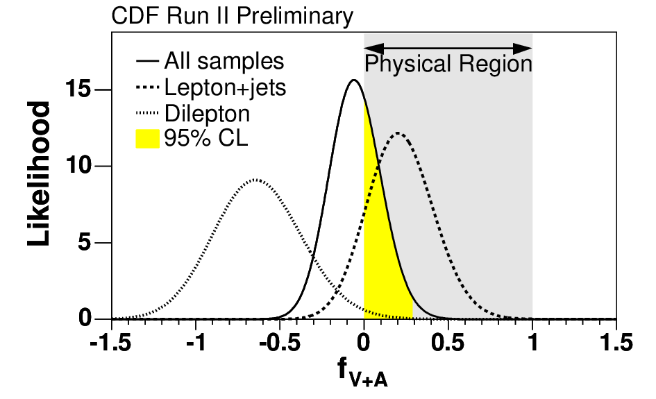
The lepton--quark invariant mass, , was used in an analysis of approximately [148]. Events with a lepton plus jets signature containing an isolated lepton, missing transverse energy and at least 3 jets with identified -jets were studied separately for one and two identified jets. In addition events with a dilepton signature containing two identified leptons with opposite electrical charge, missing transverse energy and at least 2 jets are investigated.
For each selected event the squared invariant lepton--quark mass, , is computed. In lepton plus jets events with a single identified -jet the computation is unambiguous, however, the identified -jet and the lepton are from the same top quark in only half of the cases, see Fig. 25 (left). For events with two identified -jets a two dimensional distribution of is constructed. One dimension being computed with the higher energetic -jet, the other with the lower energetic -jet. In the dilepton events the two dimensional histogram is filled twice, i.e. using each of the leptons.
The contribution of background events in the lepton plus jets samples is modelled by Alpgen events and by multijet events obtained from a control data sample. In the singly tagged sample multijet events contribute 15%, in the doubly tagged sample they are neglected. For the dilepton sample the background is described by about 50% jets from Alpgen, 30% W+jets with one jet misidentified as lepton using a single lepton sample and applying the misidentification rate. The final 20% of background are from diboson samples, and .
The signal expectation is simulated with Alpgen and Pythia assuming a top mass of for both and coupling to the boson. A binned log likelihood fit is used to extract the fraction of coupling in the top decay, . The likelihood uses Poisson probabilities to describe the expected number of events in each bin of the distributions. The parameters of the Poisson distributions are taken from the described simulation and are smeared with nuisance parameters for top pair cross-section and the total background contribution in each of three samples. These nuisance parameters are constrained to their nominal values with Gaussian probability distribution.
The procedure was verified using a large number of pseudo experiments with different nominal contributions from decays. The fit was found to be stable and unbiased. Systematic uncertainties are dominated by the uncertainty on the jet energy scale, followed by uncertainties of the background shape and normalisation as well as the limited Monte Carlo statistics.
The likelihood distributions obtained with this procedure are shown in Fig. 25 (right). The left-handed boson fraction in the top quark decay is measured to be in agreement with the Standard Model expectation of a negligible contribution. The upper limit is computed using Bayesian statistics with a flat prior for between and and yields at 95% C.L. Results for individual samples differ by at most standard deviations.
Analyses based on
The angle, , measured in the boson rest-frame between the lepton and the quark direction yields calculable distributions of this angle for each of the possible boson helicities ():
| (61) |
Measuring thus allows to reconstruct the contribution of each of these helicities in top quark decays.
CDF has used this observable in several analyses to measure the helicity fractions in top decays [149, 150]. In [149] events with an isolated lepton, missing transverse energy and at least four jets including at least one identified -jet of are investigated. Two different methods of reconstructing the full top pair kinematics are used to then compute the boson rest-frame and for each individual event.


One method recovers the unmeasured neutrino momentum from the missing transverse energy and from solving the quadratic equation following from the decay kinematics when using the nominal boson mass. This part of the analysis (for reasons that will become clear below) is called the “convolution” method. The other method (which will be called “template” method) uses a constrained kinematic fit to determine the lepton and parton momenta, where these momenta are allowed to float within the experimental uncertainties of the measured quantities. Constraints are built from the boson mass and the equality of the top and anti-top quark masses constructed from the fitted lepton and parton momenta. Both methods require an association of the measured jets to the partons of the top quark pair topology and use the quality of the constrained fit to select this assignment.
The reconstructed distribution is used in two different likelihood fits to determine the helicity fractions and either individually, fixing the other one to the Standard Model value, or simultaneously. Both methods require simulation to construct their log likelihood function. Pythia and Herwig are used to simulate Standard Model top quark pair production. Modified versions of Herwig and Madevent+Pythia [151] are used to generate samples with varied helicity fractions. The jets background is simulated with Alpgen+Herwig and normalised to the amount of data before -tagging and after removing all other background and signal events. Multijet background is taken from a control sample. Additional minor backgrounds from diboson, jets and single top quark production are taken from simulation normalised according to their theoretical cross-sections.
In the “template” method the background expectations are combined with signal templates for the three different helicity states. The helicity fractions are taken from an unbinned likelihood fit with proper correction for acceptance effects. For this method an additional cut on the scalar sum of all transverse energy was required, .
The “convolution” method uses the signal simulation to derive acceptance functions which are then convoluted with the theoretically predicted number of events in each bin of . The helicity fractions are then taken from a binned likelihood fit after subtracting the background estimation from data.
Systematic uncertainties for both methods were determined from pseudo datasets with templates modified according to the systematic effect under consideration. The jet energy scale uncertainty is among the dominating systematic effects in both methods. Only for the in the two dimensional fits the initial/final state radiation uncertainties are more important. In general the “convolution” technique yields slightly larger systematic uncertainties. Data are compared to the estimated results for the optimal fit parameters in Fig. 26. For the “convolution” method (right) the data shown are de-convoluted and compared to the pure theory prediction.
The results of the methods are combined using the BLUE method [89] with the statistical correlation between the two methods determined in pseudo experiments and the systematic uncertainties considered completely correlated. The combined results yields an improvement of about 10% compared to the individual methods. The model independent 2d fit yields
| (62) |
with a correlation of between and . Upper limits on the positive helicity fraction, are not set.
In [150] CDF investigates the dilepton channel in to determine the boson helicity fractions from . The selection requires two isolated leptons and at least two jets one of which is required to be identified as -jet.
To reconstruct the neutrino momenta are deduced by assuming the top quark pair decay kinematics with an intermediate boson. Requiring that the momenta of the corresponding decay products are compatible with the boson mass and a top quark mass of and using the missing transverse energy allows to determine the neutrino momenta up to an 8-fold ambiguity. To account for the experimental resolutions this determination is repeated with appropriately smeared input momenta. Of the eight (smeared) solutions the one that yields the smallest invariant mass is used. The distribution of measured reconstructed values is compared to templates with a binned likelihood function. Templates for the signal are obtained for various values of and using a customised Herwig generator. In addition templates for background processes of diboson, Drell-Yan and fake leptons are added to obtain the complete expectation.
Significant systematic uncertainties come from the jet energy scale and from the uncertainty of the modelling of initial and final state radiation. This special study is also suffering from limited template statistics.
In dilepton events of CDF determines the helicity fractions to be [150]
| (63) |
Additional improvements are expected from relaxing the requirement of identified -jets.
Analysis using the Matrix Element Method
In addition to the two analyses with explicit reconstruction of the top quark kinematics described above, CDF has performed an analysis that uses the Matrix Element technique to measure the longitudinal boson helicity fraction, , in of data [152, 153]. The analysis selects events with one isolated lepton, large missing transverse energy and at least four energetic jets including at least one jet identified as -jet.
For each selected event a likelihood, , to observe the measured quantities, (the lepton and jet momenta and the missing transverse energy), is computed as function of the helicity fractions. This likelihood consists of a signal term which depends on and , and a background term which is independent of these:
| (64) |
The signal and background probabilities, and , are computed by integrating the differential parton level signal and background cross-sections according to the leading order cross-sections for and jet production, respectively. These integrations account for the experimental resolutions. The product of likelihoods for all selected events is evaluated for discrete values of and . At each point the signal fraction, , is chosen to minimise the total likelihood. The result for the longitudinal helicity fraction and its statistical uncertainty are taken from the minimum of the log likelihood and its change by units.
The method is validated and calibrated using simulation for top pair signal and various background processes. Samples of various nominal values were created by reweighting the top pair events according to the expected distribution. Applying the above method to various pseudo datasets with various nominal values yields a calibration curve. The observed slope of less than one is explained by the incomplete description of signal and background each with only a single leading order matrix element. The final results are corrected with this calibration curve.
The largest systematic uncertainty for this method stems from the uncertainty in simulation. It is estimated by checking the difference between Pythia and Herwig. In addition, uncertainties due to initial and final state radiation, different PDF sets, the jet energy scale uncertainty and various other experimental effects are considered.
Using the described Matrix Element method for and assuming CDF finds
| (65) |
with a correlation of . A variation of the assumed top quark mass shifts the results for by and for by per of shift in the top quark mass from the central value [153].
DØ
The DØ collaboration has investigated a total of to determine the boson helicity fractions based on the reconstruction of the decay angle in lepton plus jets and in dilepton events [154, 155]. In the lepton plus jets events the hadronic decay is utilised to measure which helps to measure the longitudinal fraction, .
Events are selected by requiring an isolated lepton, missing transverse energy and at least 4 jets. No second lepton is allowed in the event. Dilepton events are selected with two isolated charged leptons with opposite charge, large missing transverse energy and at least two jets. Some additional cuts are applied to suppress events in the and channels and to assure a minimal transverse energy in the channel. All channels use a multivariate likelihood discriminant based on kinematic observables and the neural network -jet identification to improve the purity of the top quark pair signal.


In lepton plus jets events the decay kinematics of the top quark pairs is reconstructed using a constrained fit that determines the momenta of top quark and the boson decay products from the measured jets and lepton momenta as well as from the missing transverse energy. Only the four leading jets in are used. The fit requires the momenta of boson decay products to be consistent with the nominal boson mass and the momenta of the top quark decay products to yield a top quark mass of . Of the 12 possible jet-parton assignments the one with the highest probability of being the correct one is chosen. This probability for each association is computed using the fit as well as the output value of the neural network -tagger for the four jets and its consistency with the light or heavy quark assignment under consideration. From the chosen solution is computed from the leptonic side and a second measurement of absolute value from the hadronic side, see Fig. 27 (top and middle).
The kinematics of dilepton events can be solved assuming the top quark mass with a fourfold ambiguity. In addition the two possible assignments of the two leading jets in to the quarks are considered. For each of these solutions the decay angle is computed. To explore the full phase space consistent with the measurements, the measured jet and charged lepton momenta are fluctuated according to the detector resolution and is computed for each fluctuation. The average over all solutions and all fluctuations is computed for each jet to find two values per event. The resulting distribution for Run IIb data is shown in Fig. 27 (bottom).
The expected distribution for signal top pair events is simulated using Alpgen+Pythia with various to ratios. These samples are then reweighted to form samples corresponding to the three boson helicity states. Important backgrounds in the selected event sample are +jets and multijet events in the lepton plus jets channel, jets and jets in the dilepton samples. Backgrounds of a single weak boson with jets are simulated with Alpgen+Pythia, diboson samples are generated with Pythia. The multijet contribution is estimated from data for each bin of the distribution.
From the data and the estimated signal and background contributions a binned likelihood, , is computed for the observed data to be consistent with the sum of the backgrounds and the estimates for the three boson helicity states. The normalisation of the background is kept as a nuisance parameter with a Gaussian constraint to its nominal value. The measured helicity fractions, and , are those that minimise this likelihood.
Systematic uncertainties are evaluated in ensemble tests. Pseudo datasets are drawn from models with systematic variations and compared to the standard templates to find the resulting shift in the obtained helicity fractions. Dominating uncertainties stem from the modeling of , which are determined by exchanging the standard Alpgen+Pythia with pure Pythia, Herwig and Mc@nlo. Further significant contributions to the systematic uncertainties stem from background modeling, from the limited template statistics, from jet energy scale, jet energy calibration and jet reconstruction. An uncertainty due to the top quark mass uncertainty of is also included.
Combining the datasets of Run IIa and Run IIb, which are analysed separately, DØ finds
| (66) |
The correlation between the two numbers is about . The result shows a good consistency between the Run IIa and Run IIb datasets as well as between the dilepton and lepton plus jet channel. As for the other good agreement with the Standard Model expectation.
3.2 The CKM Element
Another aspect of the weak coupling is that of flavour changing charged currents. The Standard Model explains these through the CKM matrix that needs to be determined from experiment. The elements and of this matrix have been determined from experiment assuming the Standard Model and allow to infer [6, 156] using unitarity of a CKM matrix. Physics beyond the Standard Model may invalidate these assumptions and leave unconstrained [156]. The value of directly influences the single top quark production cross-section and the ratio between top quark decays to -quarks () and to light-quarks ( with ). Both effects have been studied by the Tevatron experiments to constrain the CKM elements related to the top quark.
3.2.1 Single Top Quark
The single top quark cross-section from Standard Model sources is proportional to . Both experiments have used this relation to convert their cross-section measurements to determinations of the CKM element [157, 158, 159]. In addition to the uncertainty of the single top quark cross-section measurement, theoretical uncertainties on the Standard Model cross-section need to be taken into account.
The combination of the CDF and DØ measurements yields a cross-section for single top quark production of [159] assuming a top quark mass of in modelling the signal efficiencies. To extract the CKM matrix element it is assumed that is much larger than and , so that the top quark decay is dominated by the decay to and no significant production through and quarks in the initial state takes place. No assumption about the unitarity of the CKM matrix is made.
With theses assumptions the analyses performed to determine the cross-section can remain unchanged for the determination of . Attributing the full deviations of the experimental result from the SM prediction to the value of the combined CDF and D0 single top quark production yields [159]:
| (67) |
3.2.2 Top Quark Pairs
In top quark pair decays the number of identified jets is used to measure the branching fraction for . This fraction can be expressed in terms of the CKM matrix elements
| (68) |
assuming that the top quark decay is restricted to Standard Model quarks.
CDF
CDF has investigated of data using both events with lepton plus jets and dilepton events [160]. For the lepton plus jets sample events are selected by requiring an isolated lepton, missing transverse momentum and four jets. Dilepton events consist of two charged leptons, missing transverse momentum and two jets. Both samples are classified according to the number of jets that are identified as jets.
The background in the lepton plus jets sample is dominated by jets events and multijet events with fake electrons. The multijet background is estimated from data using a range of control samples. The jets background is simulated using the Alpgen+Herwig generator. In the subsamples with one or more than one identified -jet, it is normalised using data before -tagging. The fraction of heavy flavour in these samples is scaled according to the Monte Carlo to data ratio in a control sample of inclusive jet events. For the description of jets events without identified jets, a neural network based on kinematic observables is used, which enriches jets background at low values and top quark pair signal at high values. The neural network was trained on Alpgen+Herwig samples. The distribution of neural network output values measured in data is compared to the simulation of jets and to fit the signal and background contribution. The shape of the multijet background is included at the rate determined above.
For the dilepton sample the main backgrounds stem from Drell-Yan, diboson and from jets events with fake leptons. The Drell-Yan background for and is simulated using Pythia normalised to the number of bosons in a mass window around . Other electroweak backgrounds are fully taken from simulation. The jets backgrounds are taken from the Alpgen+Herwig simulation applying lepton fake rates, that are determined in a complementary jet sample. A tag rate probability for generic QCD jets is used to find the contribution of fake lepton events to the various -tag subsamples.
The distribution of the number of -tags for top quark pair events depends on the branching fraction, . It is determined from events generated with Pythia and passed through full CDF detector simulation (as all simulations above).
Finally, a Poisson likelihood for the observed data to agree with the expectation is constructed as function of . Gaussian functions with nuisance parameters are used to take systematic uncertainties including correlations between the samples and the -tag bins into account. The dominant uncertainty comes from the background estimate in the -tag samples and the quark identification efficiency.
DØ
DØ has measured the top quark branching fraction, , in conjunction with the top quark pair cross-section using [162]. Events are selected for the lepton plus jets channel requiring an isolated lepton, missing transverse momentum and at least three jets. In data jets are identified using a neural network tagger.


Top quark pair signal is simulated with Pythia including samples in which one or both top quarks decay to a light quark and a boson. The dominating jets background is simulated using Alpgen+Pythia. Its heavy flavour content of the jets background was corrected according to a measurement in a control sample. The fake lepton background from multijet events is fully estimated from data. Additional smaller backgrounds from diboson, single top and jets are simulated using Pythia, SingleTop and Alpgen+Pythia, respectively, and normalised to their NLO cross-sections. All simulations are passed through the DØ detector simulation and reconstruction. In the simulation tag rate functions, determined on control samples in data, are used to describe the probability for a given jet to be identified as jet. Figure 28 (left) illustrates the probability to have zero, one or more identified jets in top quark pair events as function of the top quark branching fraction obtained from simulation.
The event samples are separated by lepton type, number of jets ( or ) and number of identified jets (, or ). The --tag sample with four or more jets is further split in bins of a topological likelihood discriminant to obtain additional separation between jets background and top quark pair signal events, c.f. Fig. 28 (middle).
To simultaneously determine the top quark pair production cross-section, , and the branching fraction, , a binned likelihood is constructed. Poisson distributions according to the expected event count as function of and is used for each sample and discriminant bin. The normalisation for jets is fixed globally by subtracting all other backgrounds as well as top quark pair estimates from data. Systematic uncertainties are included using nuisance parameters with Gaussian constraints.
For the determination of the measurement is dominated by the statistical uncertainty. Systematic uncertainties are dominated by the uncertainty of the tagging efficiency. In contrast to the CDF measurement, due to the global determination of the jets normalisation, the uncertainty on the size of this background is no significant source of uncertainty.
In of lepton plus jets data DØ obtains [162] consistent with the expectation of the Standard Model. In Fig. 28 (right) the observed number of events is compared to expectations for various values of . Limits on obtained using the Feldman-Cousins procedure yield
| (70) |
This limit is converted to a limit on the ratio of to the off-diagonal elements:
| (71) |
The only assumption entering this limit is that top quarks cannot decay to quarks other than the known Standard Model quarks. Thus it is valid even in presence of an additional generation of quarks as long as the quark is heavy enough.
3.3 Flavour Changing Neutral Currents
Flavour changing neutral currents (FCNC) do not appear in the SM at tree level and are suppressed in quantum loops [163, 164, 165, 166]. However, anomalous couplings could lead to enhancements of FCNC in the top quark sector and their observation would be a clear sign of new physics [167, 168].
The Tevatron experiments have looked for FCNC both in top quark decays [169] and in the production of (single) top quarks [170, 171, 172]. Limits on the single top production through anomalous couplings were also set with LEP and HERA data [173, 174, 175, 176, 177, 178, 179, 180].
3.3.1 Top Quark Decay through Bosons
In an investigation of data with a total luminosity of CDF looks for top quark pairs that show a flavour changing neutral current decay through a boson [169]. The analysis aims to identify events in which the boson decays leptonically and the second top quark decays through a boson into hadrons. The event selection thus looks for a pair of leptons and at least four jets. The leptons need to be of the same flavour and have opposite charge. Their invariant mass is required to be within of the boson mass. The cuts on the total transverse mass and the transverse energy of the leading and sub-leading jets were optimised in simulation. Events failing these cuts are used as control sample, events passing these cuts are split into events without any identified jet and events with at least one identified jet.
The dominant background with this selection stems from Standard Model jets production, which is simulated using Alpgen. Further but much smaller background contributions stem from Standard Model top quark pair production, and diboson production. The signal of top pairs with FCNC decay was simulated using Pythia. The events are reweighted to yield helicities of 65% longitudinal and left-handed bosons.
To separate signal from background the mass of the boson is reconstructed from two jets, the top quark mass is reconstructed by adding a third jet and a second top quark mass is reconstructed from the boson with the fourth jet. A variable is built from the differences of the reconstructed masses to the nominal boson and top quark masses, respectively. The of the jet parton assignment that yields the lowest is used to build a distribution of values.
The estimated shapes of the various backgrounds and the signal events are used as templates that are fitted to the distribution measured in data. The main parameters of the fit are the branching fraction, , and the normalisation of the dominating jets background (in the control sample). Further parameters describe the difference of the background normalisation between the signal and the control samples (with a Gaussian constraint), the quark identification fraction and the jet energy scale shift. The latter is considered to cover all shape changing affects.


The distribution of observed values is shown with the best fit of the signal and background templates in Fig. 29. Data agree well with the Standard Model templates and thus limits on the branching fraction are set. For this the Feldman-Cousins method is applied and yields at C.L. [169] The Run I result in addition sets a limit on flavour changing neutral currents in the photon plus jet mode of [181].
3.3.2 Anomalous Single Top Quark Production
While the above study of top quark decays addresses a flavour changing neutral current through the boson, investigations of the production of single top quark events can be used to restrict anomalous gluon couplings.
CDF
In an analysis of CDF looks for the production of single top quarks without additional jets, . To select such events with a leptonic top quark decay, one isolated lepton, transverse missing energy and exactly one hadronic jet are required. The jet must be identified as jet. Additional cuts are used to reduce the backgrounds without a boson as in the single top quark analyses [170].
To describe the expected background from Standard Model processes diboson and top quark pair events are simulated with Pythia and normalised to the NLO cross-sections. Single top quark events are simulated using MadGraph+Pythia [182, 183]. Finally, processes of weak vector bosons are simulated with Alpgen+Pythia. In these samples the heavy flavour contribution is enhanced according to the findings in a control sample. The total normalisation of the jets samples is taken from sideband data. The signal of FCNC production of single top quark is simulated using TopRex+Pythia [184].
Due to the large background from jet data, a neural network is employed to differentiate between FCNC and Standard Model production. Fourteen observables, which each allow a significance of more than in discriminating signal and background, were chosen as inputs to the neural network. They utilise kinematical properties of the measured quantities and the reconstructed boson as well as the output of a special flavour separation neural network. The neural network is trained on samples with equal amount of signal and background. It is then applied to the individual signal and background samples to obtain templates for all simulated physics processes considered, see Fig. 30 (left).
To determine the possible contribution of FCNC single top quark production the background templates are added according to their expected contribution and a binned maximum likelihood fit is used to measure the contribution due to FCNC production. Systematic uncertainties are parametrised in the likelihood function with Gaussian constraints. They are dominated by uncertainties on the cross-sections of the background samples normalised to NLO and the selection efficiency for signal events.


CDF finds no significant contribution of FCNC single top quark production in of data. The limit on the allowed production cross-section is set using Bayesian statistics with a flat prior for positive cross-sections and yields at C.L. [185]. This cross-section limit is converted to limits on FCNC top quark-gluon coupling constants following [186, 187]. Assuming that only one of the couplings differs from the Standard Model expectation CDF finds or . Expressed in terms of the top quark branching fraction through this processes these limits correspond to and as shown in Fig. 30 (middle and right). These small limits justify the approximation of pure Standard Model decays made in simulating signal samples above.
DØ
DØ has set limits on the FCNC anomalous couplings of the top quark in up to of data [171, 172]. The analyses investigate the singly production of a top quark in association with at least one additional jet. The event selection requires an isolated charged lepton, missing transverse momentum and at least two jets. Exactly one of the jets has to be identified as jet. With this the selection follows closely the selection used for the measurements of the single top quark production [188, 189, 190, 157].
In the most recent analysis the single top quark samples for the SM and the FCNC signal processes are simulated with the SingleTop generator [191, 192]. Background contributions from top quark pair, jets and jets production are simulated using Alpgen+Pythia and diboson production is simulated by Pythia. All samples are passed through Geant to simulate the DØ detector and then reconstructed with the standard event reconstruction. The SM samples of single top quarks, top quark pairs, jets and dibosons are normalised to the NLO (or better) cross-sections. Events from jets production are normalised to data before -tagging accounting for other simulated backgrounds and multijet background. The multijet background is described using data in which the lepton candidates fail one of the lepton identification cuts.
To separate FCNC from Standard Model prediction the method of a Bayesian neural network (BNN) is employed. A large number of variables is used as input to the neural network. These variables describe object and event kinematics, top quark reconstruction, jet width and angular correlations. For training the BNN the two FCNC processes including and couplings, respectively, are combined into a single training sample. Separate BNNs are trained for each lepton flavour and jet multiplicity. The distribution of BNN outputs observed in data agrees well with the pure SM expectation, thus limits on the allowed anomalous gluon couplings are computed.

These limits are computed using a Bayesian approach. A likelihood for the distribution of neural network outputs observed in data to occur is computed from the events expected in the Standard Model and the FCNC production of single top quark as function of the anomalous gluon couplings and . The likelihood for each bin is based on a Poisson distribution. Systematics are taken into account by smearing the Poisson parameters with a corresponding Gaussian distribution. The dominant uncertainties stem from shape changing effects like those from the jet energy scale and the modelling of quark identification. In addition normalisation uncertainties for the background simulations and the overall luminosity uncertainty give a significant contribution.
The likelihood is folded with a prior flat in the FCNC cross-sections and exclusion contours are computed as contours of equal probability that contain of the volume. The two dimensional limits on the squared couplings observed by DØ in [172] are shown in Fig. 31. One dimensional limits are obtained by integrating over one of the two anomalous couplings and yield and , corresponding to branching fractions of and . These DØ results are the currently most stringent branching fraction limits.
3.4 Top Quark Charge
The top quark’s electrical properties should be fixed by its charge. However, in reconstructing top quarks the charges of the selected objects are usually not checked. Thus an exotic charge value of is not excluded by standard analyses. Furthermore the amount of photon radiation off the top quark may a priori differ from the expection based on the top quark charge. The Tevatron experiments have searched for deviations from the SM expectation in both aspects of the top quark charge.
3.4.1 Exotic Top Quark Charge
To distinguish between the Standard Model and the exotic top quark charge it is necessary to reconstruct the charges of the top quark decay products, the boson and the quark. The boson charge can be taken from the charge of the reconstructed lepton, but finding the charge of the quark is more difficult.
DØ
DØ has performed an analysis of jets events with at least two -tagged jets in using a jet charge technique to determine the charge of the jets [193]. Semileptonic events are selected following the cross-section analysis by requiring exactly one isolated lepton, transverse missing energy and four or more jets. At least two of the jets must be identified as jets using a secondary vertex tagging algorithm.
The charge of a jet can be defined as the sum of the charges of all tracks inside the cone of that jet. In this analysis the sum has been weighted with the component of the track momenta transverse to the jet momentum, :
| (72) |
where the sums run over all tracks, , within the jet under consideration and is the charge sign of the track . Because particles may easily escape the jet cone such a jet charge fluctuates strongly from event to event, so only statistical statements can be made. It is crucial to determine the expected distribution of in the case of or quark and, because a significant fraction of charm quarks gets flagged by the secondary vertex tagger, also for the and quarks. These expected distributions, c.f. Fig. 32 (left), are derived from dijet data using a tag and probe method.


To determine the top quark charge an assignment of -jets to the leptonic or hadronic event side is necessary. This analysis uses the quality of a fit to the hypothesis, which uses the boson and top quark masses as constraints, to select the best possible assignment. The jet charge for the jet on the leptonic (hadronic) side, () is then combined with the charge of the measured lepton to define two top quark charge values per event: and . The distribution of the measured top quark charges is compared to templates simulated for the Standard Model and the exotic case, where the exotic case has been obtained by inverting the jet charge, see Fig. 32 (right). The top quark pair events are simulated using Alpgen+Pythia. The dominating jets background is simulated using Alpgen+Pythia with a normalisation to data. Multijet templates are derived from data alone. All simulated events are passed through full DØ detector simulation.
CDF, Jet Charge
The corresponding analysis by CDF investigates with events from the semileptonic and the dileptonic decay channel [195]. The former are selected requiring an isolated charged lepton, missing transverse momentum and at least four jets. Two of the jets are required to be identified jets using CDFs secondary vertex algorithm. Dilepton events are selected by asking two oppositely charged leptons, missing transverse momentum and at least two jets, one of which needs be identified as jet.
Compared to the DØ analysis the jet charge is computed slightly differently. Instead of the transverse momentum the scalar product of the jet and the track momentum is used to weigh the measured charges:
| (73) |
Depending on the sign of the identified jet is considered to stem from the or the quark. The purity of this assignment is calibrated on dijet events with two identified jets. One of the jets is required to contain a muon, that serves as tag in the tag and probe method. The resulting purity is corrected for effects due to muons from secondary decays, for meson mixing and for light or -quark jets misidentified as jets.


To compute the charge of the top and anti-top quark the jets need to be associated to the leptons. In the semileptonic channel a kinematic fit with constraints on the top quark mass and the -boson mass is used. The jet-parton association with the lowest of this fit is kept. In the dilepton channel the invariant mass of each pair of one lepton and one jet, , is computed. The combination which does not produce the largest value of is used. In both channels cuts on and , respectively, are used to enhance the purity of correct assignments.
Each event can now be classified as Standard Model like or as exotic model like. To obtain a statistical interpretation a likelihood is computed as function of the fraction of Standard Model like signal pairs, . Nuisance parameters that represent the number and purity of signal and background events are optimised for each value of . The systematic uncertainties considered include effects from the choice of parton density function, the uncertainties in the simulation of initial and final state radiation, the jet energy scale and the choice of the generator. All systematic uncertainties are included in the statistical treatment through their effect on the nuisance parameters.
Background predictions are obtained as for other CDF lepton plus jets and dilepton analyses based on a mixture of simulation and data. For this analysis each background is checked for a correlation between the charge of the signal lepton and the jet charge value of the corresponding jet. Such a correlation could occur for the semileptonic channel from the background when the lepton from the decay passes the lepton selection criteria and from single top quark events. In both cases the correlation is found to be small and consistent with zero within uncertainties.
In of data CDF finds the most likely value of the fraction of Standard Model like signal events to be . This corresponds to a -value of [195], see also Fig. 33. Because this is larger than the a priori chosen limiting probability of to falsely reject the Standard Model hypothesis, CDF claims to confirm the Standard Model hypotheses. The confidence limit corresponding to this choice is computed as . CDF computes the Bayes factor to be , which shows that this analysis with yields a much stronger exclusion of the exotic hypothesis than the DØ analysis of described above.
CDF, Soft Lepton Tag
With more data an alternative method to determine the charge of the quarks is to concentrate on the leptonic decays of the quarks. CDF applies this method on [196].
Events are selected requiring an isolated energetic lepton, missing transverse energy and at least four jets. Vetoes are applied against additional isolated energetic leptons, conversion electrons, cosmic muons, and bosons. In the four jets at least one soft lepton and one secondary vertex tag must be reconstructed. The soft lepton tag is optimised to select leptonic quark decays, , but to suppress cascade decays, . With this the charge of the quark can be deduced from the measured soft lepton charge.
To resolve the ambiguities of assigning the measured jets and energetic leptons to the (anti-)top quark decay products a kinematic fitter is applied. For the computation of the top quark charge the solution with the best fit quality is used. Only solutions which assign the tagged jets to quarks are considered. Events with a bad fit quality are rejected, if or for events with one or two tagged jet, respectively.
To estimated the expected performance of the analysis, signal events are generated with Pythia using EvtGen [197] for the decays. Background from jet events are generated using Alpgen+Pythia correcting the heavy flavour contribution by a factor derived in jet events. These samples are normalised to the data before requiring any tags. The contribution of diboson single top, jets and Drell-Yan events is considered using simulation normalised to the theoretical or experimentally measured cross-sections. Contributions from multijet events with fake leptons are estimated from data. The total background estimation is events. The purity of the charge determination is determined from these simulations and then calibrated in data using pure events.
In of data CDF finds a total of 45 events, of which are reconstructed as SM like and with the exotic charge value [196]. The statistical significance of this result is obtained by considering a large number of pseudo experiments. Figure 34 shows the expected distribution in terms of the asymmetry
| (74) |
where and are the dilution factors obtained in the calibration step for signal and background, respectively.

The SM scenario corresponds to positive values, the exotic model to negative values. In of the pseudo experiments assuming the SM the asymmetry turned out to be smaller than the measured value. Only in of the pseudo experiments assuming a fully exotic top quark showed an asymmetry larger than the measured value. From these studies the exotic charge model can be excluded at C.L.
3.4.2 Photon Radiation of Top Quarks
The top quark charge is also expected to define the amount of photon radiation off the top quark. The measurement of this process is thus a complementary way of verifying the electrical charge of the top quark. The CDF collaboration has searched for top quark pairs with an additional photon in as part of a more general search [198].
For the search of the final state, events are selected that contain an isolated energetic photon, one isolated energetic lepton, large missing transverse energy and at least three jets. One of the jets is required to be identified as -jet.
With this selection the dominant backgrounds stem from jets misidentified as photons and from light-jets misidentified as -jets. The former is estimated from data by measuring the photon fake rate in jet events as function of . This fake rate is then applied on events passing the selection without the photon requirement. Also the amount of fake -jets is determined from data and then applied to the events without the requirement of a -jet identification. Additional backgrounds including jet and diboson events are estimated using MadGraph+Pythia normalised to NLO cross-sections. MadGraph+Pythia passed through the full detector simulation and the reconstruction is also used to determine the signal selection efficiencies.
In of data CDF finds a total of 16 events which pass the described selection. The expectation including SM events is events. Attributing the full difference between the expectation and the data to the process, CDF measures the cross-section for radiation off top quark pair events of
| (75) |
with the quoted uncertainty being dominated by the statistical uncertainty. The result is in agreement with the SM expectation of [198].
3.5 Spin Correlations
At the level of the hard interaction the spins between the top and the antitop quark are correlated in top quark pair production. Because top quarks decay before they hadronise these correlations are conserved in the weak decay and thus “good” quantum-mechanic observables [199, 200, 201, 202, 203]. The degree of correlation depends on the production and decay processes. Its measurement thus probes the details of the production mechanism (when assuming a SM weak decay). The amount of correlation also depends on the reference axes used to define the top and anti-top quark spin states. At the Tevatron the spin-correlations expected in the SM are largest in the so-called off-diagonal and beam bases.
Both Tevatron experiments have measured the spin correlation of top quark pairs in different channels and using different spin bases.
3.5.1 Dilepton Channel
In the dilepton channel both experiments use the normalised double differential cross-section with respect to the angle of flight directions of the two leptons as their observable. The angle of flight, , is measured with respect to the spin quantisation axis chosen in the analysis. This double differential cross-section depends on the spin correlation coefficient :
| (76) |
In the off-diagonal and beam bases the SM predicts a correlation coefficient of about .
CDF
The CDF analysis of the dilepton channel is based on [204]. The event selection requires two leptons of opposite charge, large missing transverse energy and at least two energetic jets. A veto is applied on Drell-Yan events and on special multijet fake configurations.
The analysis selects the off-diagonal basis for the definition of the flight directions. In this basis the spin quantisation axis is defined in the centre-of-mass frame. It is defined as the direction which deviates from the direction of flight of the (anti-)top quark by the angle in clockwise direction. The value of is computed as function of the top quark velocity, , and the angle between the top quark and proton flight direction, :
| (77) |
The directions of flight with respect to the direction defined by are measured in the rest frames of the top and the anti-top quark. The analysis uses the angles obtained for the leptons () and the (anti-)-quarks ().
To reconstruct these angles in an individual event a full kinematic reconstruction of the top quark pair and its decay to is necessary. In the dilepton channel with its two neutrinos this requires the six constraints. The reconstructed boson and the top quark masses need to be consistent with their nominal values (two constraints each). In addition the sum of the transverse momenta of the reconstructed neutrinos are required to agree with the measured missing transverse energy, . Due to the quadratic nature of the corresponding equations these constraints yield up to four solutions for the unmeasured neutrino momenta, and .
To further improve the reconstruction a kinematic fit is applied that varies the reconstructed (anti-) quark energies within the experimental resolution of the jet measurements and the reconstructed sum of transverse neutrino momenta within the resolution of . Besides these resolutions the kinematic fit includes the probability densities for the distribution of the , the and the invariant mass of the top quark pair in its likelihood. Of the initially up to four solutions for the neutrino momenta, and , the one which gives the best likelihood is used to compute the flight directions in each event.
Simulations are used to determine the expected outcome of this measurement as function of the spin correlation. For the signal simulation Pythia is used. Because the Pythia samples do not contain spin correlations between the generated top quarks, the generated events are weighted proportional to according to the generated values of and . Background of dibosons and Drell-Yan are simulated using Pythia and Alpgen+Pythia, respectively. Background due to fake leptons is simulated from data with a single energetic lepton and jets. In these events one jet is artificially interpreted as a fake lepton. Both signal and background templates are smoothened by a polynomial function, where for the signal template the dependence on is kept.
The measured two-dimensional distributions of the reconstructed () and () values are now compared to the templates to determine the spin correlation coefficient using a likelihood fit. The measured value is corrected slightly according to a calibration performed on ensembles of pseudo experiments.
In of dilepton top quark pair events CDF measures the spin correlation coefficient in the off-diagonal basis to be
| (78) |
The total uncertainty is by far dominated by the statistical error. The leading systematics stems from the uncertainty on relative contribution of signal and background events. At the available statistics this results poses only a very minor constraint on the real spin correlations.
DØ
The measurement of the spin correlation by DØ uses dilepton events of up to of data [205]. Events are selected requiring two oppositely charged leptons, large missing transverse energy and at least two jets. Drell-Yan events are vetoed near the boson resonance.
In this study the flight directions in Eq. (76) are computed using the beam basis. The spin quantisation axes for the beam basis are the directions of the proton and anti-proton in the rest frame. The flight directions with respect to the quantisation axes are measured in the top and anti-top quark rest frame, respectively. DØ uses the direction of flight angles for the two measured leptons, and .
For the full reconstruction of the top quark pair kinematics DØ applies the Neutrino Weighting Method described in the context of top quark mass measurement in Sect. 2.3.1. For the spin correlation measurement the weight, , is computed for a fixed top quark mass of , but scanning possible values of the flight angles to find its dependence on the product , i.e. for each event . For further analysis the mean, , of the weight function in each event is used:
| (79) |
The distribution of values found in the selected events is now compared to templates obtained from simulation. Signal templates for a range of values are obtained by reweighting Pythia. Templates for the events is generated with Alpgen+Pythia, while for diboson processes Pythia is used alone. Both background types are normalised to the theoretical cross-sections. To enhance the bad simulation of the boson distribution, a reweighting of these events has been applied. The measured spin correlation parameter is obtained by a binned likelihood fit of the templates to the measured data.
DØ has studied the performance of this method in ensembles of pseudo experiments using various nominal values of . This calibration is used in the Feldman-Cousins procedure [161, 6] to obtain the final results. Using dilepton events DØ determines the spin correlation coefficient in the beam axis
| (80) |
The uncertainty is dominated by statistics. The leading systematic uncertainty is found to come from signal modelling. This includes a dependence on the assumed top quark mass as well as differences observed when replacing Pythia by Alpgen+Pythia or Mc@nlo. The observed spin correlation is in slight tension with the SM expectation of about .
3.5.2 Lepton plus Jets Channel
CDF has also determined top quark spin correlations in the semileptonic decay channel [206, 207]. In events with one energetic lepton, large missing transverse momentum and at least 4 jet are selected; at least one of the jets is required to be identified as -quark jet.
This analysis uses the the beam and the helicity bases. The spin quantisation axes are defined in the rest frame. For the beam basis the beam direction is used, for the helicity basis the (anti-)top quark directions are taken. Then the angles between the flight directions of the top quark decay products, , and the quantisation axis are reconstructed in the (anti-)top quark rest frame. The analysis considers the lepton direction, , the bottom quark from the hadronic top quark decay, , and the down-like quark, .
For the determination of these angles the full event kinematics of the top quark pair decay is reconstructed using a kinematic fitter which constrains the top quark mass to . Only events with a reasonable fit quality are considered in the analysis. In the following analysis the distributions of the of the reconstructed angles are compared to templates. For the reconstructed value of the jet which is closest to the -jet in the rest frame is used. This is found to be the down-type quark in about of the cases.
For the analysis of the angles in the helicity basis, samples of the four possible helicity combinations of the top and anti-top quark are generated with a modified version of Herwig. From these four combinations, equal helicity and opposite helicity samples are obtained assuming parity and conservation. In the analysis of the angles with respect to the beam basis the signal samples are obtained by reweighting Pythia events according to the generated decay angles. In addition templates for the expected background are produced, including multijet, jets and diboson events.
To determine the spin correlation the two dimensional distribution of vs. is fitted with the described templates using a binned likelihood fit. The contribution of the same spin and the opposite spin templates are allowed to float freely, the background contribution is allowed to float but constrained to the expectation within its errors. The determined fractional contribution of the opposite spin contribution, , is converted to the spin correlation coefficient using .
In CDF determines the spin correlation in the helicity and in the beam bases to be
| (81) |
The measurement is clearly dominated by the limited statistical uncertainty. Of the systematic uncertainties the uncertainty on the signal modelling is by far dominating.
3.6 Charge Forward Backward Asymmetry
At the Tevatron the initial state of proton anti-proton is not an eigenstate under charge conjugation. Thus in principle also the final state may change under this operation. In QCD, however, such a charge asymmetry appears only at next-to-leading order and arises mainly from interference between contributions symmetric and anti-symmetric under the exchange of top and anti-top quarks [208, 209, 210, 211, 212].
Experimentally, CDF and DØ investigated forward backward asymmetries [213, 214, 215, 216]
| (82) |
where and are the number of events observed in the forward and backward direction, respectively. The forward and backward directions are either defined in the laboratory frame, i.e. according to the sign of the rapidity of the top quark, , or can be defined in the frame where the top quark pair system rests along the beam axis, i.e. according to the sign of the rapidity difference between top and anti-top quark, . The two different definitions of forward and backward yield two different asymmetries that are labelled and according to their rest frame of definition. In the Standard Model at NLO asymmetries are expected to be and , respectively [217], but at NNLO significant corrections are predicted for the contributions from [218].
The smallness of the asymmetries expected within the Standard Model make them a sensitive probe for new physics.


CDF
The CDF collaboration has investigated up to of data and measures both charge asymmetries defined above from top quark pairs with semileptonic decay [214, 216]. The event selection requires an isolated lepton, missing transverse energy and at least four hadronic jets, one of which must be identified as jet.
The top and anti-top quark kinematics are reconstructed from the jet momenta, the lepton momentum and the missing transverse momentum using mass constraints from the boson and the top quark. The reconstructed values of these masses are constrained by the nominal values of and and tagged jets are assigned to quarks only [216]. Of the possible jet parton assignments the one with the best fit probability is taken. The rapidity of the hadronically decayed (anti-)top quark, , is multiplied by minus the charge, , of the lepton to obtain the top quark rapidity: . For the frame asymmetry, the rapidity difference is computed as , with and as above and being the rapidity of the leptonically decayed (anti-)top quark.
The NLO Standard Model expectation of top quark pair production is done with Mcfm [219] and the next-to-leading order generator Mc@nlo [220] which contain a small asymmetry. Leading order signal simulation without asymmetry from Pythia is used to check for any detector or selection asymmetry. The dominating background events of jets are simulated with Alpgen+Pythia, diboson backgrounds and single top quark events are simulated with Pythia and Madevent, respectively. The normalisation of the jets background and contributions from misreconstructed multijet events are estimated from data.
The uncorrected rapidity and rapidity difference distributions measured in data are compared to the expectations in Fig. 35. These distributions differ from the true particle level shape due to acceptance and reconstruction effects. After background subtraction CDF derives the particle level distributions inverting the acceptance efficiencies and migration probability matrices as derived from Pythia simulation with zero asymmetry using a reduced number of only four bins. The final asymmetries are computed from these unfolded distributions.
The dominating systematic uncertainties are the background normalisation and shape. For the amount of initial and final state radiation contributes significantly, while for the jet energy scale is the next leading uncertainty. Further uncertainties from the parton distribution functions, due to colour reconnection and the MC generator are considered.
The final asymmetries measured in the update to of CDF data are [216]:
| (83) |
These values are somewhat larger than the and expected in the Standard Model at NLO, respectively, but agree within two standard deviations.
CDF also investigated the dependence of the asymmetry on several other topological and kinematic properties. Considering the two ranges of yields:
| (84) |
Clearly, the deviation from the expectation is driven by the effect at large rapidity differences.
The functional dependence of the asymmetry on the invariant mass of the top quark pairs is shown in Fig. 35 (right). Separating this result in two bins yields
| (85) |
The events with high invariant mass show a deviation standard deviations from the NLO prediction obtained with Mcfm.
CDF completes their study by verifying that the asymmetries are consistent with CP conservation by separately considering events with positively and negatively charged leptons. The slightly enhanced asymmetry observed in the inclusive measurement thus seems to stem from effects at large rapidity difference and high invariant mass of the top quark pair system.
DØ
The DØ collaboration has investigated up to of data to measure in semileptonic top quark pair events [213, 215]. The event selection requires exactly one isolated lepton, missing transverse momentum and at least four jets, the hardest of which must have . At least one of the jets is required to be identified as jet with DØ’s neural network tagger.
The top quark pair kinematics is reconstructed by fitting the momenta of the top quark decay products to the measured jet and lepton momenta and the missing transverse energy with constraints on the reconstructed boson and top quark mass to and , respectively. Only the jets and the remaining three leading jets are used. The possible jet parton assignments are reduced by assigning identified jets only to quarks. In the final analysis only the assignment with the best fit probability is used. The rapidity difference with the correct sign is determined from the rapidities reconstructed of the leptonic and the hadronic side ( and ) and the lepton charge, : .
To estimate the dominant background of jets production a set of observables well described by the simulation is used to construct a likelihood discriminant that does not depend on . The expected shape of top quark pair signal and the jets background in the distribution of the discriminant and on the asymmetry is determined from Mc@nlo and Alpgen+Pythia simulation, respectively, passed through DØ detector simulation and reconstruction. The effect of multijets events on the asymmetry and the discriminant is determined from data that fail the lepton identification. Other backgrounds were checked to have negligible effects.
The final reconstructed asymmetry, , in signal events is determined by maximising the combined likelihood of the observed discriminant distribution and the distribution of the sign of as function of the signal and background contributions and of the signal asymmetry. The dominant systematic uncertainties on the asymmetry are the jet energy calibration and the asymmetry reconstructed in jets events. All of them are much smaller than the statistical uncertainty.
In of data DØ finds a final observed asymmetry [215] of
| (86) |
To keep the result model independent and in contrast to the CDF results this number is not corrected for acceptance and resolution effects. Instead it needs to be compared to a theory prediction for the phase space region accepted in this analysis which is corrected for dilution effects. For NLO QCD and the cuts used in this analysis DØ evaluates . Thus as for CDF this result corresponds to an asymmetry that is slightly higher than expected in NLO QCD, but not by more than two standard deviations.

In addition to the QCD expectation in the published analysis [213] DØ provides a parameterised procedure to compute the asymmetry expected for an arbitrary model of new physics. As an example the measurement’s sensitivity to top quark pair production via a heavy neutral boson, , with couplings proportional to that of the Standard Model boson is studied. Pythia is used to obtain a prediction of this kind of top quark pair production and due to the parity violating decay yields large observable asymmetries of to depending on the assumed boson mass. Limits on the possible fraction of heavy production are determined as function of the boson mass using the Feldman-Cousins approach. These limits are shown in Fig. 36 and can be applied to wide resonance by averaging the appropriate mass range.
3.7 Differential Cross-Section
Measurements of the differential cross-sections of top quark pair production can be used to verify the production mechanism assumed in the Standard Model. Due to the required unfolding these measurements are especially cumbersome. The CDF collaboration has measured the differential cross-section with respect to the invariant top quark pair mass, , using of data [221]. The event selection requests a lepton with high transverse momentum, large missing transverse momentum and at least four jets. At least one of the jets needs to be identified as -jet.
The invariant mass of the top quark pairs is reconstructed from the four-momenta of the four leading jets in , the four momentum of the lepton and the missing transverse energy. The -component of the neutrino is not reconstructed but used as if it was zero [222].
The dominating background in this selection stems from jets production. Its kinematics simulated with Alpgen+Pythia correcting heavy flavour contribution for differences between data and Monte Carlo. The required normalisation is measured in data before applying the -jet requirement [223]. Multijet background is extrapolated from data with low missing transverse momentum. The smaller backgrounds of diboson, jets and single top quark is fully taken from simulation using Pythia, Alpgen+Pythia and MadGraph, respectively. All simulated events are passed through the CDF detector simulation and reconstruction.
To obtain the differential cross-section from the background subtracted distribution of observed values, acceptance effects and smearing effects from the reconstruction need to be corrected for. The required acceptance correction is computed from signal simulation with Pythia. Factors to correct for differences between data and Monte Carlo observed in control samples are applied for the lepton identification and -jet identification rates. The distortions of the reconstructed distribution are unfolded using using the singular value decomposition [224] of the response matrix that is obtained from simulations.
Relevant systematic uncertainties arise from the background normalisation, the acceptance, parton density distributions, the used Monte Carlo generator and jet energy scale. The relative contributions of the uncertainties strongly depend on . To reduce the uncertainty on the jet energy scale an in-situ calibration of the jet energy scale is performed. This uses the invariant dijet mass reconstructed from the two non--tagged jets most consistent with .
The differential cross-section obtained in of data using the semileptonic decay mode is shown in Fig. 37 [221]. The consistency with the Standard Model expectation is computed using Anderson-Darling statistics [225]. The observed -value is 0.28, showing good agreement with the Standard Model.


Finding no evidence for physics beyond the Standard Model limits on gravitons in a Randall-Sundrum model [226] decaying to top quarks are set using the CLs method [227, 228]. Signal is modelled with MadGraph+Pythia assuming a first resonance with a mass of . The Anderson-Darling statistics is used as test statistics in the CLs method. For the ratio of the warping parameter over the Planck mass CDF finds at C.L, see Fig. 38.
The invariant top quark pair mass was used in further analyses by both CDF and DØ to search for new physics. These results are described in Section 4.4.
3.8 Gluon Production vs. Quark Production
Top pair production at the Tevatron with takes place either through quark anti-quark annihilation or through gluon fusion. The former is expected to dominate with the gluon fusion contributing about . Due to the large uncertainties of the large- gluon density in the proton the exact size of the gluon contribution is rather uncertain [30, 31, 34].
Two properties of the two production processes allow to separate them and to measure their relative contributions. Close to threshold the spin states of the gluon fusion are , , while the annihilation yields , [229]. This yields angular correlations between the charged leptons in the dilepton channel. Alternatively one can exploit the difference in the amount of gluon radiation from quarks and gluons: The gluon fusion processes are expected to contain more particles from initial state radiation. CDF has used both features to measure the gluon fraction of top quark pair production.
3.8.1 Angular Correlation Methods
Dilepton Channel
CDF has investigated of data with an event signature of top quark pair dilepton events [230]. The selection requires two oppositely charged leptons, at least one of which must be isolated, and at least two jets. The scalar sum of the lepton and jets transverse energies must exceed . Additional cuts are placed to reject cosmic particles, leptons from photon conversion and boson events.
The azimuthal angle between the two leptons is measured in each event. Then a template method is used to measure the fractional contribution of the different production mechanisms. The expected behaviour of signal events is simulated using Herwig with the top quark mass set to and the CTEQ5L parton distribution function. Pythia and Mc@nlo are used in systematic studies. Backgrounds are dominated by diboson production and boson events with tauonic decay. These are simulated by Pythia. In addition the background from events with only one true lepton and a jet misidentified as lepton are described using data. All simulated events are passed through the full CDF detector simulation and reconstruction.
The angular distributions obtained for events produced by annihilation and fusion and the sum of backgrounds are separately fitted with smooth functions, that then serve as signal and background templates.

The measured fraction of top quark pairs produced through gluon fusion is obtained from an unbinned likelihood fit of these templates to the observed data, c.f. Fig. 39 (left). Systematic uncertainties include uncertainties on the template shapes, the acceptance differences between annihilation and gluon fusion, the used matrix element, initial and final state radiation and PDF uncertainties. The uncertainties are determined as function of the nominal gluon production fraction and several of them may contribute up to . All systematic uncertainties are included in the determination of the Feldman-Cousins band, see Fig. 39 (right), which is used to obtain the final result with errors.
In the investigated of dilepton events CDF obtains a gluon fusion fraction of [230]. The total uncertainty is dominated by statistical uncertainties and is not yet able to restrict the theoretical uncertainties on the gluon fusion production.
Lepton plus Jets Channel
Angular correlations are also used by CDF in an analysis of with lepton plus jets events [231]. The events are required to contain one energetic lepton, large missing transverse energy and at least four jets. One of the jets is required to be identified as jet through the presence of a secondary vertex.
In each event the decay chain of the top quark pair decay is reconstructed from the four leading jets using a kinematic fit with constraints on the boson and the top quark mass, c.f. Section 2.2.1. Only jet parton assignments which associate the tagged jet(s) with a quark are considered. The one with the best fit quality is used for further analysis.
From the reconstructed top quark pair decay, eight observables are used to feed a neural network that is trained to distinguish between and production. The observables are the (cosine of the) angle between the top quark momentum and the beam direction of the incoming proton, the top quark velocity and the (cosines of the) six angles of the top quark decay product as defined in the off-diagonal spin basis, c.f. Section 3.5. The first two observables are contributing about one third of the total sensitivity, each. The six decay angles yield the remaining third.
The neural network is trained separately for events with one and with more than one identified jet. Simulation of the two signal production processes is done with Herwig, the dominant background of jets is generated with Alpgen+Herwig. The generated events are passed through the full detector simulation and reconstruction chain of CDF. To obtain the measured production fraction, , templates for the neural network output are constructed from the simulation as function of and a likelihood to observe the measured data as function of is maximised. The Feldman-Cousins approach [161, 6] is applied to restrict the final result to the physically allowed range.
To determine the systematic uncertainties various pseudo experiments with systematically varied signal and/or background templates are studied. The deviation of obtained in these samples from the standard template result is considered as systematic uncertainty. The dominant uncertainty is found to stem from background shape and composition as well as from the differences between leading and next-to-leading order simulation of the signal.
In of lepton plus jets events CDF is able to set limits on the production fraction of at C.L. [231]. This method yields independent information, but is not as sensitive as the following method.
3.8.2 Soft Track Method
Another method that CDF applies to measure the fraction of top quark pair production through gluon fusion relies on differences that occur because gluons have a higher probability to radiate than quarks [232]. The analysis is based on top quark pairs with semileptonic decays in of CDF data.
As sensitive observable the average number of soft tracks per event, , with in the central detector region is used. In simulation this is shown to have linear relation to the average number of gluons, , in the hard process. This relation is calibrated on two samples with different gluon content: jets events for low gluon content and dijet for high gluon content. jet events are used as cross-check.
The dijet event sample for calibration is selected requiring a leading jet with transverse momentum between and and a second recoiling jet with . Vetoes are applied on lepton candidates and missing transverse energy. The jets sample is selected requiring an isolated lepton, large missing transverse energy. For the signal top quark pair sample in addition at least four jets are required. At least one of these jets must be identified as -jet. In the jets and top quark pair samples vetoes on additional lepton candidates and on leptons consistent with photon conversion or cosmic rays are applied.
After calibration of the relation between and , the fraction of events with a high gluon content, , is determined using a binned likelihood fit. The fit result is corrected according to the expected background contribution. The fraction of events with high gluon content in the background, , is extrapolated from the jets sample with up to three jets to the four or more jet sample. The expected amount of background in the selected signal sample is determined following the neural network based method in [223]. The obtained high gluon content in top quark pair events, , in a last step is corrected for the differences in acceptance between the gluon fusion and the annihilation processes.
The systematic uncertainties of this measurement are dominated by uncertainties of the calibration procedure and were determined by varying the corresponding parameters in the analysis.
In the dataset of CDF determines a gluon fusion fraction of top quark pair production in semileptonic events of [232]. This number corresponds to an upper limit of at C.L, well in agreement with the Standard Model expectations. Also this measurement is statistically limited. A combination of this result with the result of the Angular Correlation Method described in the previous section yields an about improvement on the upper limit [231].
3.9 Top Quark Width and Lifetime
The top quark width and its lifetime are related by Heisenberg uncertainty principle. In the Standard Model the top quark width is expected to be corresponding to a very short lifetime of about . Experimentally, these predictions have been challenged for deviations in very different analyses. CDF constrains the lifetime from the distribution of reconstructed top quark mass values and from the distribution of lepton track impact parameters. DØ combines the measured branching fraction and the single top -channel cross-section to measure the top quark width.
3.9.1 Top Quark Mass Distribution
The limit on the top quark width was obtained by CDF from the the distribution of reconstructed top quark mass values from top quark pairs decaying to lepton plus jets in up to of data [233, 234]. After selecting events with one lepton, large missing transverse momentum and at least four jets. One of the jets is required to be identified as -jet.
In these events the top quark mass is reconstructed using a kinematic fit that determines the four-momenta of the top quark decay productions from the measured jet and lepton momenta and the transverse missing energy. The fit uses constraints that force the boson decay products to build the boson mass within the width of the boson and the reconstructed top and anti-top quark masses to be equal within the top quark width. In the ambiguous association of jets to partons identified -jets are only associated to -quarks. Of the remaining associations and the two solutions for the neutrino -momentum, the one with the best is used. It was checked that the use of the constraint of the equality of the top quark masses width does not destroy the sensitivity to the true width.
To find the measured value of the top quark width the distribution of top quark masses reconstructed with the best association in each event is compared to parametrised templates with varying nominal width. Templates for top quark pair signal events were generated using Pythia with [234]. Background contributions of jets are modelled Alpgen+Pythia. Multijet contributions from data with non-isolated leptons. Single top quark and diboson events are simulated with MadGraph. The template distributions for discrete values of the nominal top quark width are parametrised to obtain smooth template functions that can now be interpreted as probability densities. The measured top quark width is determined in an unbinned likelihood fit.
Recently, in addition to the reconstructed top quark mass, the invariant mass of the jets assigned to the hadronic decay is considered as an observable. This allows a simultaneous fit of the top quark width and the jet energy scale [234].
The Feldman-Cousins approach [161, 6] is used to determine the final result excluding the unphysical values of negative widths that may occur in the fit. The jet resolution followed by colour reconnection effects yield the biggest single contribution to the systematic uncertainties. are propagated to the final Feldman-Cousins band by convoluting their effects with the fitted width function.
Including all systematics this CDF analysis of yields an upper limit of the top quark width at C.L. which corresponds to . At C.L. the top quark width is determined as [234].
3.9.2 Lepton Impact Parameter
The limit from the lepton track impact parameter distribution was obtained by CDF using lepton plus jets events in of data [235]. Events are selected requiring one isolated lepton, missing transverse energy and at least three jets. At least one of the jets has to be identified as -jet. The lepton track needs to be reconstructed with at least three - positions in the CDF silicon tracker.
The lepton impact parameter, , chosen as observable in this measurement is defined as the smallest distance between the collision point and the lepton track in the transverse projection. The collision point is computed as the position of the beam line in the transverse plane at the reconstructed position of the primary vertex.
The distribution of lepton impact parameters expected in an ideal detector for various top quark lifetimes is simulated with Pythia. The resolution of the CDF detector is measured in Drell-Yan data near the boson resonance and used to derive the templates for the real detector expectation. The dominant backgrounds like jets consist of prompt leptons, which are described by the zero lifetime template. But the distribution of multijet events, backgrounds with leptons and electrons from photon conversions need to be modelled. Multijets and electron conversions are modelled from control samples in data. Backgrounds with leptons are modelled using Herwig.
From these templates a likelihood as function of is built. The maximal likelihood is obtained from the template. Systematic uncertainties on the signal and background systematics are computed with correspondingly varied templates and are dominated from the uncertainty on the detector resolution for prompt leptons. The Feldman-Cousins approach is used to determine the observed limit of at C.L.
3.9.3 Branching fraction and single top cross-section
The total width of the top quark can be written as the ratio of the partial width for the decay and the corresponding branching fraction:
| (87) |
DØ measures the top quark width by relating the partial width and branching fraction to the results of two independent analyses [236]. The branching fraction in the denominator is equal to the branching fraction ratio, , measured from top quark pairs (c.f. Section 3.2.2). This assumes that the top quark always decays to a -boson plus a quark. The partial width is derived from the single top production cross-section which is proportional to . When considering only the -channel cross-section, , this proportionality is valid also in the presence of anomalous couplings in the -vertex. Thus the partial width is determined as
| (88) |
where the superscript SM indicates the Standard Model expectations. As the total width is by definition larger than the partial width, a lower bound of at 95% C.L. can be set from the -channel production cross-section [190] alone. In the combination of the partial width with the branching fraction systematics are classified and treated as either fully correlated or uncorrelated. They are dominated by uncertainties in the background description and the description of the -jet identification in the input analyses.
3.10 Outlook to LHC
Within the SM the interaction properties of the top quark are fully defined once the top quark mass is known. The verification of the predicted properties establishes the top quark as the particle expected in the SM. Huge progress has been made in the last years in experimentally verifying the expectations. Measurements of the boson helicity, the CKM element and searches for FCNC confirm the expected weak interaction properties. The electric charge has been challenged and the strong interaction properties have been verified in differential cross-section measurements, in a verification of the contribution of gluon fusion processes and also in the forward backward charge asymmetry. First tests of the spin structure and determinations of the top quark width complete the current picture. All current results are compatible with the SM expectations, a single deviation of appears in the charge asymmetry at high .
Despite the great progress, the precision of the experimental knowledge of interaction properties of the top quark is still limited. Many results have not yet reached a precision of . As a consequence of the experimental progress even the more precise results, like the boson helicity and the measurement of , are statistically limited.
The near future will see updates of the results with the yet unanalysed Tevatron data to a total . In addition the LHC schedule envisions to collect of proton-proton collisions at . The LHC experiments will then have about twice as many top quark pairs as the Tevatron and even three times as many single top quarks. For the top quark pairs the production through gluon fusion and for the single top quark the -channel production will dominate. When systematic uncertainties can be controlled similarly well as at the Tevatron, the LHC results on this dataset will still be limited by statistics.
Only the update of the LHC to the design centre-of-mass energy of will provide sufficiently many top quarks to enter an area of precision measurements in the verification of top quark interactions.
An important exception to these statements is the measurement of the forward-backward asymmetry, which cannot be measured in collisions. Instead related asymmetries need to be studied [237, 211, 217, 238, 239]. These measurements will probably require large luminosity as only quark annihilation diagrams contribute to the asymmetries.
4 New Particles in Top Quark Events
The phenomenology of the top quark may also be altered by particles that are not expected within the Standard Model, but in one of the many models of new physics. Such particles beyond the Standard Model may occur in the top quark production or its decay, depending on the specific model or its parameters. Some models of new physics also contain new particles with signatures that are very similar to the Standard Model top quark. The Tevatron experiments have checked for all these different extensions of the Standard Model in the top quark sector.
This subsection will actually start with a process that is expected in the Standard Model though at very low rate: associated Higgs production. In some models of new physics this process is expected to be enhanced. Then particles beyond the Standard Model in the top quark decay will be discussed. Finally, searches for the production of particles that look like the top quark but are not are described.
4.1 Associated Higgs Boson Production,
Top quark pair production may be associated by the production of a Higgs boson. For parameters where Higgs bosons dominantly decay to bottom quark pairs, i.e. low Higgs masses, this associated production is a possibility to measure the top quark Yukawa coupling. While the corresponding cross-section in the Standard Model is too low to allow a Higgs discovery in this channel alone, it still contributes to the combination of the Standard Model Higgs searches. In some models including new physics an enhancement of production is expected [240, 241, 242].
DØ
DØ performed an analysis searching for associated Higgs production in events with a lepton ( or ) missing transverse energy and at least four jets [243]. The analysis uses the scalar sum of transverse momenta, , the number of jets and the number of jets identified as -jets to discriminate the Standard Model backgrounds and top pair production containing no Higgs from the signal.
Signal events are simulated using Pythia. For production pure Pythia simulation was compared to Alpgen+Pythia simulation. Due to the difference between the two simulations a uncertainty was assigned to the contribution of through QCD processes. Background from jets events is simulated with Alpgen+Pythia and normalised to data. Multijet background was completely estimated from data. Smaller backgrounds are taken from simulation normalised to NLO cross-sections.
In the investigation of the observed data agree with the Standard Model expectations within statistical and systematic uncertainties [243]. To compute limits signal and background contributions are fitted to the data for a background only assumption and for a signal plus background assumption. Limits on are then derived using the CLs method [227, 228] for Higgs masses between and .
For the cross-section limit corresponds to about 60 times the Standard Model value. While this allows to exclude unexpectedly large Higgs boson production in association with the top quark, its contribution to the Standard Model Higgs search remains small.
4.2 Charged Higgs Boson


Particles beyond the Standard Model in the final state of top quark pair events may alter the branching fractions of the various top quark decay channels and modify the kinematic properties of the final state.
Charged Higgs bosons appear in many extentions of the Standard Model due to the need for an additional Higgs doublet with a separate vacuum expectation value. These models are characterised by the ratio of the vacuum expectation values of the two Higgs doublets, . A charged Higgs boson can replace the boson in top quark decays. Because charged Higgs bosons have different branching fractions than bosons this alters the branching fractions to the various top quark pair decay channels. If its mass is different from the it also modifies the kinematic properties of the top quark pair final state.


In the Minimal Supersymmetric Standard Model (MSSM) [245] the decay at low is dominated by hadronic decay to at low Higgs boson masses and to for Higgs boson masses above about . For larger than about a leptonic decay to dominates, c.f. Fig. 40. The figure also shows the expected branching fraction of which is especially large for very low and very high and rather small in the intermediate range.
CDF
CDF has performed two analyses with different approaches. An analysis based on uses the CDF cross-section measurements in various channels and recasts the interpretation to obtain limits on the charged Higgs boson production. A second more recent analysis on investigates the kinematic differences between lepton plus jets events from top quark pair production with Standard Model decay and those including charged Higgs boson decays.
Recast of Top Quark Pair Cross-Section
To obtain limits on a possible charged Higgs boson contribution in top quark decay CDF utilises cross-section measurements performed in the lepton plus jets channel (with exactly one -tag or two or more tags), the dilepton channel and the plus lepton channel [244]. Care is taken to avoid overlap between the various channels. Beside the Standard Model decays of a top quark through a boson, four decay modes through the charged Higgs boson are considered: , , and . The latter has a non-negligible contribution at intermediate values of .
Selection efficiencies are taken from simulation of top quark pair events for various masses of the top quark, the charged and neutral Higgs boson, . The simulation takes the dependence of the width of the top quark and the charged Higgs boson into account. The production cross-section is kept at its Standard Model value for : .
The event counts observed in data in the four channels are compared to the expectations in three different ways. For specific benchmarks of the MSSM a Bayesian approach is used to set limits on . This analysis uses a flat prior on within the theoretically allowed range. These limits are computed for various values of the charged Higgs boson mass and five different parameter benchmarks. Figure 41 (left) shows the results for one specific benchmark.
For the high region dominates in a large fraction of the MSSM parameter space. Setting the branching fraction of to , limits on the charged Higgs contribution to top quark decays are set using Bayesian statistics. A flat prior for between 0 and 1 is used. For charged Higgs boson masses between and CDF can exclude at 95% C.L.
Finally, a more model independent limit is computed by scanning the full range of possible charged Higgs boson decays. For all five decay modes considered the branching fraction is scanned in 21 steps, assuring that the sum of branching fractions adds to one. Limits on are computed for each combination. The least restrictive limit is quoted. Also this analysis is repeated for various charged Higgs boson masses. The limits obtained in this more general approach, shown in Fig. 41 (right), exclude only very high contributions of charged Higgs bosons to top quark decays of above approximately to , depending on the charged Higgs boson mass.
Investigation of Kinematic Differences
At low , where the charged Higgs boson can also decay to , CDF used the invariant dijet mass to search for a possible contribution in top quark pair events [246]. Lepton plus jet events are selected requiring at least two of the four leading jets in to be -tagged. The four leading jets are used in a kinematic fit that requires consistency of the fitted lepton and neutrino momenta with the boson mass and reconstructed top quark masses to be . The dijet mass of the hadronic decay remains unconstrained. The jet parton assignment with the best is used and the charged Higgs boson mass is reconstructed from the non--tagged of the 4 leading jets. For events with more than jets the th jet is added to its closest neighbour if their to improve the dijet mass resolution.
Background events are dominated by top quark pair production with Standard Model decay. Further processes included are jets, jets, diboson, single top quark and multijet events. Except for multijet events the backgrounds are estimated from simulation. The normalisation for jets taken from data, for the others it is taken from theory. The multijet background is fully determined from data.


To determine a possible contribution of charged Higgs boson in the decay of top quark pair production a binned likelihood fit is performed. The likelihood is constructed with templates for the backgrounds and using the branching fraction of top quark to charged Higgs bosons, the number of top quark pair events and the number of background events as parameters. The number of background events is constrained within the uncertainty to the expectation. The observed dijet mass distribution and the fitted background composition is shown in Fig. 42 including a charged Higgs boson contribution of 10%.
Systematic uncertainties are computed by fitting pseudo data created from systematically varied templates with the standard unshifted templates. The change of the branching ratio due to the systematic variation is taken as systematic uncertainty for each variation considered. These uncertainties are included to a final likelihood by convoluting a Gaussian distribution to the original likelihood. Systematic uncertainties are dominated by the signal modeling that is derived from replacing the default Pythia sample of events by a Herwig sample. For Higgs boson masses close to the boson mass the jet energy scale uncertainty becomes dominant.
For various assumed Higgs boson masses 95%CL limits on the branching fraction are determined by integrating the likelihood distribution to 95% of its total. As shown in Fig. 43 limits between about 10% and 30% can be set depending on the mass of the charged Higgs, consistent with the expected limits for pure Standard Model top quark decays. This result is less model dependent than the above CDF limits, but not as strict within the models used above.
DØ
The DØ collaboration searched for a light charged Higgs boson contribution in top quark decay by reinterpreting the cross-section measurements in various decay channels and for heavy charged Higgs boson contributing to single top quark production.
Charged Higgs Boson in Top Quark Decay


In the search for a light charged Higgs boson in top quark decay DØ uses the cross-section analyses for lepton plus jets, dilepton and lepton plus tau decay channels, with lepton refering to and only [126, 248, 247]. The channels are kept disjoint and further separated into subsamples depending on the number of jets, the number of tags and the lepton type. The number of expected events for each of the subsamples is computed from simulation with Pythia including the Standard Model decays and decays of the top quark to a leptophobic or a tauonic charged Higgs boson and charged Higgs boson masses between and .
A likelihood for the observed data is built each of the two models given the number of expected events as function of the branching fraction . The observed is extracted by maximising the likelihood.
In a first iteration the production cross-section is fixed at a value of . Limits are set according to the Feldman-Cousins procedure including systematic uncertainties. The systematic uncertainties in this method are dominated by uncertainties due to the assumed top quark pair cross-section, the luminosity and -jet identification. The resulting limits obtained with of data exclude a branching fraction above around for the pure leptophobic model and above for the tauonic model, c.f. Fig. 44 [247].

In a second iteration the production cross-section is treated as a free parameter and determined simultaneously with the limits on charged Higgs production, see Fig. 44. This reduces the assumptions made in the determination of the limit. In addition the result is much less sensitive to the luminosity. In this method the description of multijet background becomes the largest systematic uncertainty. Such a two dimensional fit is only possible for the tauonic decay model where this analysis includes channels that get enhanced in the presence of a charged Higgs and others that get depleted. In this channel the sensitivity enhances by more than for low Higgs boson masses [247].
DØ further discusses the implication for various supersymmetric models and sets exclusion limits on these models in the plane of model parameters and .
Charged Higgs Boson in Single Top Quark Production
Heavy charged Higgs bosons can not only occur in the decay of top quarks but may contribute to single top quark production. Their signature is identical to Standard Model -channel single top quark production, but may have a resonant structure in the invariant mass distribution of its decay products, the top and the bottom quarks.

Following their single top quark analysis, DØ selects events with an isolated lepton, missing transverse energy and exactly two jets, one of which is required to be identified as -jet [249]. Background estimation for jets and production is simulated using Alpgen. Standard Model single top quark production is modelled using SingleTop [191, 192]. Charged Higgs boson signal events are simulated with a narrow width for the charged Higgs boson using CompHEP. Three types of two Higgs doublet models (2HDM) are considered. In the Type I 2HDM one doublet gives mass to all fermions; in the Type II model one doublet gives mass to the -type quarks (and neutrinos), the other to the -type quarks and charged leptons. This model is realised in the MSSM. In the Type III 2HDM both doublets contribute to the masses of all fermions. Due to the different couplings the cross-section of single top quark production in these 3 models is quite different.

Standard Model and charged Higgs boson production of single top quarks is separated by reconstructing the invariant mass of the two jets and the boson. This distribution shows good agreement between data and the Standard Model expectation, see Fig. 46. Bayesian statistics is used to set limits on the allowed cross-section for single top quark production through a charged Higgs boson. For the Type I 2HDM some region in vs. can be excluded, c.f. Fig. 47, a significant fraction of phase space is not accessible by the analysis in its current form due to the restriction to small decay widths [249].
4.3 Heavy Charged Vector Boson,
New charged gauge bosons, , are expected in extensions of the Standard Model with additional gauge symmetries and in supersymmetric models, see e.g. [6, 245]. Its couplings may be to left-handed fermions, like for the Standard Model boson, or include right-handed fermions. In general a mixture of these two options is possible. If the boson has left handed couplings, it will have a sizeable interference with the SM boson [250]. For purely right-handed couplings, a leptonic decay may only occur when the right-handed neutrinos are lighter than the boson. In this case the decay to a top and bottom quark is an interesting channel to perform direct searches for such bosons.
Both CDF and DØ search for various types of bosons decaying to pairs in conjunction with their single top quark analyses. The main discriminating observable is the reconstructed invariant mass of the decay products, which was also utilised to search for a heavy charged Higgs boson, c.f. Section 4.2.
DØ
DØ has published a search for a heavy boson with decay to top and bottom quarks using [251]. The event selection follows the single top quark analysis and requires one isolated lepton, missing transverse momentum and two or three jets, one of which must be identified as -jet.


The invariant mass, , of the bottom and the top quark decay products is computed from the measured four-momenta of the leading two jets, the charged lepton and the neutrino. The transverse momentum of the neutrino is identified with the transverse missing momentum, its -component infered by solving choosing the solution with the smaller .
The distributions expected within the Standard Model from a combination of simulation and data. Single top quark and top quark pair production is generated with SingleTop and Alpgen+Pythia normalised to their theoretical cross-sections. +jets background is generated with Alpgen+Pythia and normalised to data before -tagging in a way that it includes diboson backgrounds. Also the +heavy flavour fraction is derived from data. Multijet background is fully taken from data. Samples of boson events with masses up to are generated in conjunction with the single top quark samples taking interferences with the boson into account that are present for the left-handed bosons. Because of this interference the Standard Model single top quark production in the -channel is treated as part of the signal in the search for bosons.
The distribution of reconstructed measured by DØ agrees with the expectation from the Standard Model. Limits on a possible contribution from bosons decaying to top and bottom quarks are derived as a function of assuming couplings like in the Standard Model, though possibly to right handed fermions. DØ uses the Bayesian approach with a flat non-negative prior on the cross-section times branching fraction. Expected and observed results are shown in Fig. 48.

Comparing upper limits on the boson cross-section times branching fraction to top and bottom quark to the NLO theory predictions [252] excludes left-handed bosons with . If only hadronic decays are allowed the right handed boson is excluded for , when leptonic decays are also possible the limit is .
Without assuming the coupling strength the Bayesian approach is used to determine a limit on the size of this coupling relative to the Standard Model, see Fig. 49. These limits assume no interference between the Standard Model and the bosons.
In computing the above limits systematic uncertainties are included. They include effects due to uncertainties on the integrated luminosity, the theoretical cross-sections, branchings fraction, object identification efficiencies, trigger efficiencies, fragmentation models, jet energy scale and heavy flavour simulation.
CDF
In an investigation of of data [253] CDF selects jets events requiring one lepton (, ) isolated from jets, missing transverse energy and two or three energetic jets. At least one of the jets must be tagged as -jet.
In these events the neutrino momentum, , is infered from the missing transverse momentum and by solving for the longitudinal component of the neutrino. The boson mass, , is set to its nominal value, is the measured lepton momentum. In case of complex solutions CDF assigns the real part of the solution to the longitudinal neutrino momentum. The invariant mass of the lepton, the neutrino and the two leading jets, , is then used as a discriminating observable.
The distribution expected within the Standard Model is computed from a combination of simulation and data. The contribution of events containing a real boson is taken from simulation. jets samples are normalised to data before -tagging using a scale factor to correct the heavy flavour contribution to fit the observation in 1jet data. The other samples are normalised to their theoretical expectation. The identification of heavy flavour jets is estimated from simulation and corrected with a scale factor. Misidentification of light flavour jets is computed from mis-tag rate functions. The contribution from events without real bosons are estimated from events with electrons that pass only a subset of the full electron identification and thus are enriched with jets misidentified as electrons.

boson signal events are simulated using Pythia for boson masses between and with fermion couplings identical to the Standard Model boson. When the right-handed boson is heavier than the right-handed neutrinos, the branching fraction to is corrected according to the additional decay modes.
Limits are constructed according to the CLs method [227, 228]. Probabilities are computed from pseudo experiments which are generated including variations due to systematic uncertainties. The dominating systematic uncertainties are the jet energy scale and the scale factor used to account for differences between simulation and data in the -tagging algorithm of CDF.
Limits on the boson production cross-section are set as a function of assuming the Standard Model coupling strength. These are converted to mass limits by comparison to the corresponding theoretical expectation and yield for bosons which decay leptonically and for . For the more general case that the coupling is a priori unknown the coupling strength, , relative to the Standard Model coupling, , is constrained. Limits are computed from the above analysis as function of the assumed . The observed and expected limits derived by CDF for and are shown in Fig. 50 and 51.

4.4 Resonant Top Quark Pair Production
Due to the fast decay of the top quark, no resonant production of top quark pairs is expected within the Standard Model. However, unknown heavy resonances decaying to top quark pairs may add a resonant part to the Standard Model production mechanism. Resonant production is possible for massive -like bosons in extended gauge theories [254], Kaluza-Klein states of the gluon or boson [255, 256], axigluons [257], Topcolor [258, 259], and other theories beyond the Standard Model. Independent of the exact model, such resonant production could be visible in the reconstructed invariant mass.
CDF
CDF has employed several different techniques to search for resonances in the invariant mass distribution. All analyses use a very similar event selection: an isolated lepton, missing transverse energy and four or more jets. One analysis (the Matrix Element plus Template method) is also applied to the full hadronic channel selecting six or seven jets. Their main difference is the method to reconstruct the invariant mass distribution.
Constrained Fit plus Template
The method that uses the least assumptions reconstructs the invariant mass using a constrained fit [260] and is performed requiring at least one identified jet. In the fit the final state lepton and quark momenta are determined from the measured lepton momentum, the missing transverse energy (which is assumed to stem from the unseen neutrino) and the measured jet momenta. Constraints are imposed that require the sum of neutrino and lepton momenta as well as the two light quark momenta to be consistent with the boson mass. In addition these pairs in combination with one quark need be consistent with the top quark mass of 175 GeV. The fitted momenta may vary within the experimental resolution of their assigned measurement and the mass constraints are varied within the natural widths of the boson and the top quark, respectively. The fit thus assumes the lepton plus jets decay topology of top quark pair events.

Of the multiple jet parton assignments the one with the best from the fit is used to compute the top quark pair invariant mass for each event. The expected distribution of this observable is dominated by Standard Model top quark pair events which are simulated using Herwig. Further backgrounds like jets, misidentified multijet events, diboson and single top quark events are modelled with combination of simulation and control data.
Templates for a resonant production of top quark pairs are simulated using Pythia for resonance masses between and . The resonance couplings are proportional to those of a Standard Model boson. The width of this boson was kept at . The observed invariant top quark pair mass distribution is compared to the distribution expected from the Standard Model in Fig. 52.
From the expected distributions CDF constructs a likelihood for the expected bin content of the distribution of the invariant top quark pair mass as function of the resonant production cross-section time branching ratio, , the number of Standard Model top quark pairs and the number of non- events. Nuisance parameters with Gaussian constraints are used to implement the effect of systematic uncertainties. These include uncertainties that affect the relative background normalisation and the luminosity, the uncertainty of the jet energy scale and the shape change due to the top quark mass uncertainty. Minor contributions come from varying the PDFs between CTEQ6M [36] and MRST [261] parametrisations and the uncertainty on the strength of initial and final state radiation.

To find the upper limits the maxima of the likelihood as function of is integrated to the point where the integral reaches 95% of its area. This is done for each assumed resonance mass between and in steps. Expected and observed limits are shown in Fig. 53. At high resonance masses the observed limits exclude a resonant top quark pair production with at 95% C.L. A production through leptophobic Topcolor assisted Technicolor is excluded for resonance masses up to .
Matrix Element plus Template
The resolution of the reconstructed invariant top quark pair mass can be improved by assuming additional information. In an analysis of CDF employed the Matrix Element technique to reconstruct the invariant mass distribution that is used to search for resonant production in lepton plus jets events [262]. Following the mass analysis [93] described in Section 2.2.3, for each event a probability density, , is computed to find the momenta of the top quark pair decay products (4 quarks, charged lepton and neutrino, ) given the observed quantities, . This probability is computed from the parton density functions, the theoretical Matrix Element for Standard Model top quark pair production and decay and jet transfer functions that fold in the detector resolution. It is converted to a probability density for the top quark pair invariant mass using
| (89) |
The result for all possible jet-parton assignments is summed, before the mean value is computed and taken as the reconstructed invariant top quark pair mass for the event under consideration. Here the -tagging information is used to reduce the number of allowed jet parton assignments. The events are not required to contain -tagged jets in the event selection.

Template distributions for Standard Model and resonant processes are derived from Pythia, jets events from Alpgen+Herwig including full detector simulation. As a resonance signal a boson with a width of was generated. The multijet background template was taken from data. The Standard Model samples and diboson samples are normalised to the theoretical cross-section, while the sum of multijet and jet samples are scaled to fit the observed data and depend on the assumed signal contribution. The resulting expected distribution compared to the observed data is shown in Fig. 54.

The possible contribution from a resonant top quark pair production is computed using Bayesian statistics. The posterior probability density is build from a likelihood that implements Poissonian expectations in each bin. The parameters of the Poisson distribution are smeared with Gaussians according to the systematic uncertainties. Finally, the posterior probability density is convoluted with a flat prior in . The uncertainties of the Standard Model top quark pair production cross-section, the jet energy scale and the variation of initial and final state gluon radiation have the largest impact on the resulting limits.
The events observed by CDF in of data show no evidence for resonant top quark pair production and upper limits are derived for as shown in Fig. 55. A comparison to the leptophobic Topcolor assisted Technicolor model yield an exclusion of this model for at 95%C.L. Using additional assumptions about the kinematics through the matrix element thus allows to exclude slightly higher boson masses despite using less data.

The Matrix Element plus Template method was also applied in the all hadronic decay channel using of CDF data with six or seven jets [263]. Top quark pair events are enriched with a neural net event selection and jet identification. The dominant multijet background is described with a data driven method from events without the identification requirement.
No evidence for resonant top quark pair production is found. CDF computed upper limits on the resonant production cross-section time branching fraction, , as shown in Fig. 56. In the leptophobic Topcolor assisted Technicolor model resonance masses of are excluded at 95%C.L.
Dynamical Likelihood Method with Massive Gluon interpretation
Another analysis of CDF is based on the dynamical likelihood method (DLM, see also Section 2.2.3). It investigates of data with an isolated lepton, missing transverse energy and exactly four reconstructed jets [264]. In contrast to the previously described analysis the invariant top quark pair mass is reconstructed without using the production part of the matrix element in the construction of the probability densities in Eq. (89). This avoids a bias towards the Standard Model production mechanism. The resulting distribution and the corresponding Standard Model expectation is shown in Fig. 57.


The distribution is then used to search for a new colour-octet particle, called a massive gluon. An unbinned likelihood fit based on the production matrix elements with and without massive gluon contribution is used to extract the possible coupling strengths of such a massive gluon contributing to the top quark pair production. The likelihood is computed for various masses and widths of the massive gluon. The systematic uncertainties are incorporated in the likelihood calculation. Jet energy scale and top mass uncertainties are the largest contribution to the total uncertainty on the fitted coupling, .
The observed data agree with the Standard Model expectation within . This agreement is cross-checked by reconstructing the top quark -distribution, which is also found to be in agreement with the Standard Model expectation. Limits on the possible coupling strength of a massive gluon, , contributing to the top quark pair production are set at 95% C.L. for various values of the width, as function of the mass, . Figure 58 shows the expected and observed limits for two choices of the massive gluon width.
DØ
DØ investigated the invariant mass distribution of top quark pairs in up to of lepton plus jets events [265, 266, 267]. The event selection requires an isolated lepton, transverse missing momentum and at least three jets. At least one of the jets needs to be identified as jet. Signal simulation is created for various resonance masses between and . Separated resonance samples were generated with couplings proportional to Standard Model boson couplings, with pure vector couplings and with pure axial-vector couplings. The width of the resonances was chosen to be of their mass, which is much smaller than the detector resolution.
The top quark pair invariant mass, , is reconstructed directly from the reconstructed physics objects. A constrained kinematic fit is not applied. Instead the momentum of the neutrino is reconstructed from the transverse missing energy, , which is identified with the transverse momentum of the neutrino and by solving for the -component of the neutrino momentum. and are the four-momenta of the lepton and the neutrino, respectively.


The invariant mass can then be computed without any assumptions about a jet-parton assignment that is needed in constrained fits. Compared to the constrained fit reconstruction, applied in an earlier analysis, this gives better performance at high resonance masses and in addition allows the inclusion of 3 jets events. The expected distribution of Standard Model processes and the measured data is shown in Fig. 59. For comparison a resonance with a mass of is shown at the cross-section expected in the Topcolor assisted Technicolor model used for reference.

Cross-sections for resonant production are evaluated with Bayesian statistics using a non-zero flat prior (for positive values) of the resonant top quark pair cross-section time branching fraction, . A Poisson distribution is assumed for the number of events observed in each bin of the likelihood. The prior for the combined signal acceptance and background yields is a multivariate Gaussian with uncertainties and correlations described by a covariance matrix. The measured correspond to the maximum of the Bayesian posterior probability density, limits are set at the point where the integral of the posterior probability density from zero reaches of its total. Expected limits are obtained by applying the procedure when assuming that the observed result corresponded to the Standard Model expectation. The limits obtained for the -like, vector and axial-vector resonances are found to agree with each other, thus these limits are valid for a general (colour neutral) narrow resonance.
These expected limits were used to optimise major analysis cuts and the -tag working point. In Fig. 60 (left) the expected limits are used to visualise the effect of the various systematics by including one after another. The lowest curve corresponds to a purely statistical limit. Adding the jet energy uncertainty shows that this uncertainty mainly contributes at medium resonance masses. The various object identification efficiencies and the luminosity are added. They essentially scale like the background shape. Finally the effect of the top quark mass is included and it is most important at low resonance masses [268].
In of DØ data the observed cross-sections are close to zero for all considered resonance masses, as shown in Fig. 60 (right). The largest deviation (around ) corresponds to a little more than standard deviations. Thus limits are set on the as function of the assumed resonance mass, . The excluded values range from about for low mass resonances to less then for the highest considered resonance mass of . The benchmark Topcolor assisted Technicolor model can be excluded for resonance masses of at CL.
4.5 Admixture of Stop Quarks
A final very fundamental question that may be asked in the context of top quark physics beyond the Standard Model is, whether the events that are considered to be top quarks actually are all top quarks or whether some additional unknown new particle is hiding in the selected data. The top quark’s supersymmetric partners, the stop quarks and , are possible candidates in such a scenario.
4.5.1 DØ, Lepton plus Jets
The stop quark decay modes to neutralino and top quark, , or through chargino and quark, , both yield a final state with a neutralino, a quark and a boson, . The neutralino is the lightest supersymmetric particle in many models and is stable if -parity is conserved. Then it escapes the detector and the experimental signature of stop quark pair production differs from that of semileptonic top quark pair events only by the additional contribution to the missing transverse energy from the neutralino.
DØ has searched for a contribution of such stop quark pair production in the semileptonic channel in data with [269, 270]. Semileptonic events were selected following the corresponding cross-section analysis by looking for isolated leptons ( and ), missing transverse energy and four or more jets. At least one of the jets was required to be identified as -jet using DØ’s neural network algorithm.
To describe the Standard Model expectation a mixture of data and simulation is employed. The description of top quark pair production (and of further minor backgrounds) is taken fully from simulation normalised to the corresponding theoretical cross-sections. For jets the kinematics is taken from simulation, but the normalisation is taken from data. Multijet background is fully estimated from data. As signal the lighter of the two stop quarks, , is considered. Production of is simulated for various combinations of stop quark and chargino masses, . For the sake of this analysis the stop quark mass was assumed to be less or equal to the top quark mass. The neutralino mass was chosen to be close to the experimental limit.


To detect a possible contribution of stop quark pairs the differences between stop quark pair events and Standard Model top quark pair production kinematic variables are combined into a likelihood, . The kinematic variables considered include the transverse momentum of the (leading) jet, distances between leading jet and lepton or leading other jet. Additional variables were reconstructed by applying a constrained fit. In this fit reconstructed physics objects (lepton, missing transverse energy and jets) are assigned to the decay products of an assumed semileptonic top quark pair event and the measured quantities are allowed to vary within their experimental resolution to fulfil additional constraints. It was required that the boson mass is consistent with the invariant mass of the jets assigned to the two light quarks as well as with the invariant mass of the lepton with the neutrino. The masses of the reconstructed top quark pairs were constrained to be equal. Of the possible jet parton assignments only the one with the best was used. From the constrained fits observables the angle between the -quarks and the beam axis in the rest frame, the invariant mass, the distances between the ’s and the same-side or opposite-side bosons and the reconstructed top quark mass are considered. The likelihood was derived for each combination separately and the selection of variables used has been optimised each time. Figure 61 shows the separation power of the reconstructed top quark mass and the full likelihood for the case of , and the comparison to the observed data.
To determine limits on the possible contribution of stop quark pair production in the selected channel Bayesian statistics is employed using a non-zero flat prior for positive values of the stop quark pair cross-section. A Poisson distribution is assumed for the number of events observed in each bin of the likelihood. The prior for the combined signal acceptance and background yields is a multivariate Gaussian with uncertainties and correlations described by a covariance matrix. The systematic uncertainty is dominated by the uncertainties on the theoretical cross-section of top quark pair production, on the selection efficiencies and the luminosity determination. Figure 62 shows the expected and observed limits on the stop quark pair production cross-section compared to the MSSM prediction for various values of and . The theoretically expected stop quark signal cross-section in the MSSM is smaller than the experimental limits for all parameter points considered.
4.5.2 CDF, Dilepton
CDF has searched for a contribution of stop quarks in the dilepton channel using upto of data [271]. The dilepton event signature was chosen to cover chargino decay modes to that do not involve an intermediate boson and thus may not have a corresponding hadronic decay to build semileptonic events.
CDF collected data using an inclusive high- trigger and selects events with 2 leptons, one of which needs to be isolated from calorimeter energies not associated to that lepton. The events are required to have missing transverse energy and at least 2 jets. A boson veto is applied for and events. To suppress the leading background, Standard Model top quark pair events, from the selected event a cut in the plane of vs. plane is applied, where is the product of the azimuthal angles between the leading jets and the two leptons: . This cut reduces top quark pair production by a factor of 2, but reduces stop quark by approximately only.
The Standard Model background expectation is modelled using simulation and control data. Simulation of top quark pair production and other minor backgrounds are normalised to their NLO cross-section. jets samples are normalised to control data of low missing transverse energy near the -pole separately for events with and without -tags. To model events with faked leptons that may stem from other top quark pair decay channels, from jets or from multijet events, parametrised lepton fake rates are derived from a large sample of generic jets. These fake rates are applied to events with lepton plus electron or muon like events to find the contribution of fakes in the signal region.
To describe signal events stop quark pair production is simulated with various combinations of neutralino, chargino and stop quark masses lighter than the top quark mass. Generated samples are interpolated through a template morphing technique to obtain any combination of masses within the generated range.
The reconstructed stop quark mass is used to distinguish a stop quark signal from Standard Model backgrounds including top quark pair production. The stop quark mass, , is determined following an extention of the dilepton neutrino weighting technique.


-jets are assigned to their proper lepton based on jet-lepton invariant mass quantities. A correct assignment is reached in to of the cases with both -jets being the leading 2 jets. Neutralino and neutrino are considered as a single, though massive, pseudo particle. For given directions of the pseudo particles the particle momenta are determined with a fit to the measured quantities using constraints on the assumed pseudo particle mass, the assumed chargino mass and the equality of the two stop quark masses. The reconstructed stop quark mass is computed as weighted average of the fitted stop quark masses, where the average is computed over all values of , with weights of . The expected and observed distributions for two choices of parameters are shown in Fig. 63.
The combination of reconstructed stop quark mass templates from the signal and the various background components is fitted to data. Systematic uncertainties enter the fit through nuisance parameters, signal and background contributions are allowed to vary within their rate uncertainties and the shape may vary according to CDFs morphing technique. The ratio of the likelihoods is used to do the limit-setting according to the CLs technique [227, 228].


Depending on the dilepton branching ratio limits are set in the stop quark vs. neutralino mass plane. Figure 64 shows the results for two choices of parameters. These limits are derived using only very few assumptions, these are (a) is the LSP and , and are heavy, (b) and (c) . Thus the limits are valid over a large range of SUSY parameter space.
4.6 Heavy Top-like Quark,
Another class of hypothetical particles that may hide in samples usually considered as top quarks are new heavy quarks, in this context usually called quark. These new particles a considered to decay to and thus show a signature very similar to that of top quarks.
Heavy top-like quarks appear in a large number of new physics models: A fourth generation of fermions [272], Little Higgs models [273] and more named in [274]. Strong bounds are placed on such models by electroweak precision data, but for special parameters the effects of the fourth generation particles on electroweak observables compensate. Among other settings a small mass splitting between the fourth -type quark, , and its isospin partner, , is preferred, i.e. [272]. Especially, when the new top-like quark is very heavy, it should be distinguishable from Standard Model top production in kinematic observables. A search for such heavy top-like quarks has been performed by both Tevatron experiments.
CDF
The CDF collaboration has repeatedly analysed their samples of lepton plus jets events to search for a new top-like quark. The published result uses [274] and the preliminary updated results of data [275]. The analyses consider pair production of a new quark heavier than the top quark and with a subsequent decay to . The event selection requires exactly one isolated lepton, large missing transverse energy and at least four energetic jets.
The dominant Standard Model processes that pass this selection are top quark pair production which is simulated using Pythia, jets events which are simulated using Alpgen+Herwig or Pythia and normalised to data and multijet events which are modelled from data with reversed lepton identification. Minor backgrounds like jets and diboson events are considered to be described by the jets simulation. The simulation of signal is performed using Pythia.


As the quark decay chain is the same as the top quark decay chain a constrained fit to the kinematic properties is performed. The momenta of the quarks and leptons from the quark and the following boson decays are fitted to the observed transverse momenta. The constraints require that the boson decay products form the nominal mass and that the decay products of the quark yield the same mass on the hadronic and the leptonic side. Of the 12 different jet-parton assignments CDF chooses the one with the best of the fit. The corresponding mass from the fit, , is used as one observable to separate signal from background. The second observable is the total transverse energy, , i.e. the sum of transverse energies of the observed jets, the lepton and the missing transverse energy. The choices explicitly avoid imposing -quark tagging requirements. The expected and observed individual distributions are shown in Fig. 65.
The signal and background shapes in the two dimensional - plane are used to construct a likelihood for the observed data as function of the assumed quark cross-section, . Then Baysian statistics is employed to compute expected and observed limits on that are shown in Fig. 66.

Systematic uncertainties are implemented through nuisance parameters that are constrained in the fit with a Gaussian function to their nominal value within their expected uncertainty. The jet energy scale is named as one of the largest uncertainties. In addition uncertainties on the scale used in simulating jets, on initial state and final state radiation, on the multijet background determination, the integrated luminosity, the lepton identification, the parton density functions and the expected quark cross-section as function of the quark mass are considered.
The limits on quark pair production cross-section, , determined in this search for a new top-like heavy quark are compared to the theoretical prediction [31]. Assuming CDF concludes that a pair production can be excluded for at 95%CL. However, for masses of the observed limit is worse than the expectation by about two standard deviations, which indicates a surplus of data for that range.
DØ
The DØ collaboration has searched for a heavy top like quark with a decay to a -boson and a quark using of data [276]. Events are selected which show an isolated lepton, large missing transverse energy and at least four jets.
The dominating backgrounds from Standard Model processes are top quark pair and jets production, which are simulated using Alpgen+Pythia. The simulation and additional smaller backgrounds from diboson and -boson production are normalised to the expected Standard Model cross-sections. The normalisation of the jets contribution is determined below. The contribution of multijet background faking a lepton is derived from a sample with loosened lepton selection. Signal simulation is obtained from Pythia for 13 different mass values using a fixed decay width of .
Also DØ uses a reconstructed -quark invariant mass and the scalar sum of transverse momenta to distinguish the -quark signal from the Standard Model backgrounds. The -quark invariant mass is derived in a full event reconstruction assuming the expected decay . In this reconstruction the momenta of the assumed decay products are fitted to the reconstructed measured objects applying constraints that enforce the mass of the intermediate -bosons and equality of the initial and masses. All possible associations of the four leading jets in to the quarks are considered. To select the best association in addition to the fit a term is computed that prefers low transverse momenta for the reconstructed -quark. The -mass reconstructed, , with the association that minimises is taken for further analysis.


Two dimensional distributions of vs. are used to fit the data compositions with free jets and signal normalisations, c.f. Fig. 67. This is done for all 13 -quark mass hypotheses and for a background only hypothesis. DØ uses the CLs method [227, 228] with a Poisson likelihood as the test statistics to determine the cross-section limits. DØ includes several systematic uncertainties affecting the normalisation of the fixed background contributions as well as shape changing effects in the limit calculation. Of the normalisation uncertainties the luminosity uncertainty gives the largest single contribution.
The limits on a -quark production cross-section observed by DØ in [276] and the corresponding expectations are shown in Fig. 68 as function of the hypothetical mass. By comparing to the theoretical prediction [31] DØ excludes heavy top like quarks with masses less than at 95% C.L. Over almost the full range the observed limit stays behind the expected limit indicating a surplus of data in the -signal range. Correspondingly the expected mass exclusion of is not reached.

4.7 Outlook to LHC
Due to the high mass of the top quark it has been speculated that the top quark may play a special role in particle physics. Many models of new physics involve new particles that may occur in top quark production or decay. The Tevatron experiments have investigated a wide range of options for such new particles in top quark events and also looked for particles with signatures very similar to that of top quarks. So far no significant deviation has been found.
In the near future the LHC is scheduled to deliver at least at . With such a dataset the LHC experiments will have roughly twice as many top quark pairs and three times as many single top quarks as the Tevatron with the expected . The benefit of this data, however, depends on the process in which the new particle appears.
Searches for new particles that occur in the top quark decay, like e.g. a charged Higgs boson, will benefit directly from the increased dataset and yield results competitive to those of the Tevatron. Searches for new particles that occur in the production like, or bosons or a quark, will benefit from the larger centre-of-mass energy. The cross-sections of such processes, however, scale with the corresponding parton luminosity, which increases much more for the gluon than for the quark luminosity. Particles like the boson that can by produced only by quark-antiquark annihilation thus will have less signal events in than the Tevatron will have in the expected . Such analyses will still extend the Tevatron results to the phase space areas opened with the higher centre-of-mass energy. Finally, the search for a boson produced in the single top quark -channel, like the , will suffer from the comparably moderate increase of the corresponding cross-section and thus require more statistics at the LHC to become competitive to the Tevatron results.
With the design LHC at the larger production cross-section and the enlarged phase space will again extend the results significantly. An ATLAS study assuming collisions at and a luminosity of [144] has considered the potential for discovering resonant top quark pair production through a narrow boson. A significant degradation of the selection efficiency is expected at high top pair invariant masses because the top quark decay products join into the same jet more and more often. Given the performance visible in the first results shown at conferences from LHC experiments searches for new physics in top quark events will greatly advance at each new energy reached by the LHC after collecting a moderate luminosity of e.g. .
5 Conclusions
More than fifteen years after the discovery of the top quark the experimental verification of the properties expected in the Standard Model has reached a first level of maturity. With the luminosity delivered by the Tevatron accelerator in its Run II to the CDF and DØ experiments many top quark properties have been challenged and contributions for new particles have been searched for.
The top quark mass measurements, with the elaborate statistical methods of the Matrix Element technique, have now reached a statistical precision of less than and experimental systematics of making the top quark mass the most precisely known mass of all quarks. This precision significantly exceeds the precision goals of about of the Tevatron Run II programme set for [47, 277]. Despite the low branching fraction of the dileptonic channel, even results in this channel alone now have achieved an experimental precision exceeding this goal. In order to reach these small uncertainties, it was important to constrain the jet energy scale, leading to the dominating uncertainty, in-situ to data. Unfortunately, the experimental precision on the top quark mass is currently not matched by a corresponding theoretical understanding. The uncertainty of the mass definition used in the simulations that the experiments apply to calibrate their measurements is not known better than to the order of . This complicates the comparison of the top quark mass results, e.g. with other electroweak precision data, and is a fundamental problem also for the LHC programme. Discussions on these issues have started between the experimental, the generator and the theoretical community in order to collect the information needed to overcome this issue. The development of methods that precisely determine the mass in well defined definitions is an important problem in current top quark physics.
Many interaction properties have been challenged by the Tevatron experiment in the recent years. Production properties such as the quark and gluon induced production rates, the electrical charge and the various decay properties did not show significant deviation from the expectation and thus confirm that we observe the top quark expected in the SM. The structure of the weak top quark decay has been tested in the boson helicity measurements to the 5% level and weak decays through flavour changing neutral currents are constrained to be below the 4% level. The largest deviation () from the SM was found in the forward backward charge asymmetry at high . While the sheer number of tests documents a great progress the precision of these measurements is generally limited by statistics. Searches for new particles have been performed in events with top quark like signatures. Neither specific searches for supersymmetric top quark partners, for charged Higgs bosons nor searches for bosons, quarks or generic resonances found any significant deviations from the SM expectations. Also these studies are limited by the statistics available so far.
The Tevatron is planned to be shutdown in autumn 2011. Until then it is expected to increase the total integrated luminosity for the CDF and DØ experiments to more than . The analyses of the Tevatron take advantage of several years of optimising the reconstruction of the recorded events. Thus further updates of existing analyses, but also investigation of yet untested properties can be expected. In addition the LHC has started to operate at well above that of the Tevatron centre-of-mass energy. It is expected to deliver an integrated luminosity of at least throughout 2011. Due to the increased collision energy at the LHC the top production cross-sections are significantly higher than at the Tevatron. With the LHC experiments will have collected about twice as many top quark pairs and three times as many single top quarks than the Tevatron experiments at .
Given the impressive performance of the LHC experiments shown at recent conferences it is natural to assume that the systematic uncertainties can be controlled comparably well as at the Tevatron experiments, if not better. We will thus see a plethora of competitive results from the LHC experiments. Clearly some searches profit from the increased phase space and will be dominated by the LHC. There are also results where the Tevatron has an advantage, like the charge asymmetry and the single top quark search, however, most results will be comparable. Also at the LHC many will be statistically limited which makes it useful to foresee a combination of the results.
After an update to the design LHC with proton-proton collisions at the field will be taken over by the LHC experiments. With a top quark pair cross-section which is times higher than at the Tevatron and dominant backgrounds like jets and jets increasing only by factors of about the LHC will become a real top quark factory. Again many searches for new particles will profit from the enlarged phase space. Measurements of interaction properties and searches for new particles in top quark decays will become limited by systematics after only a short running at design luminosity. At the same time with the huge expected statistics new types of measurement methods on rare subsamples will become feasible. For the top quark mass methods using leptonic decays or using events with very high top quark momentum will have very different experimental and theoretical uncertainties. Such alternative methods with different systematic uncertainties will contribute to the combination of results. And may even help to solve the puzzle of the meaning of the top quark mass.
Acknowledgments
The author would like to thank his colleagues in the DØ and CDF collaborations for their support in the preparation of this review. Special thanks belong to Frank Fiedler, Lina Galtieri, Alexander Grohsjean, Klaus Hamacher, Michele Weber and Wolfgang Wagner for valuable discussions about experimental details and to Werner Bernreuther, André Hoang, Sven Moch and Peter Uwer for detailed support and suggestions on theoretical questions. Finally, I would like to thank Stefan Tapprogge for valuable suggestions in the preparation of this work.
References
- (1) S. L. Glashow, “Partial symmetries of weak interactions,” Nucl. Phys. 22 (1961) 579.
- (2) J. Goldstone, A. Salam, and S. Weinberg, “Broken symmetries,” Phys. Rev. 127 (1962) 965.
- (3) S. Weinberg, “A model of leptons,” Phys. Rev. Lett. 19 (1967) 1264.
- (4) H. Fritzsch, M. Gell-Mann, and H. Leutwyler, “Advantages of the color octet gluon picture,” Phys. Lett. B47 (1973) 365.
- (5) P. W. Higgs, “Broken symmetries, massless particles and gauge fields,” Phys. Lett. 12 (1964) 132.
- (6) Particle Data Group, K. Nakamura et. al., “Review of particle physics,” J. Phys. G37 (2010) 075021.
- (7) Boomerang, P. de Bernardis et. al., “A flat universe from high-resolution maps of the cosmic microwave background radiation,” Nature 404 (2000) 955–959, arXiv:astro-ph/0004404.
- (8) WMAP, D. N. Spergel et. al., “First year Wilkinson Microwave Anisotropy Probe (WMAP) observations: Determination of cosmological parameters,” Astrophys. J. Suppl. 148 (2003) 175, arXiv:astro-ph/0302209.
- (9) SNLS, P. Astier et. al., “The Supernova Legacy Survey: Measurement of , and from the first year data set,” Astron. Astrophys. 447 (2006) 31–48, arXiv:astro-ph/0510447.
- (10) WMAP, D. N. Spergel et. al., “Wilkinson Microwave Anisotropy Probe (WMAP) three year results: Implications for cosmology,” Astrophys. J. Suppl. 170 (2007) 377, arXiv:astro-ph/0603449.
- (11) CDF, F. Abe et. al., “Observation of top quark production in collisions,” Phys. Rev. Lett. 74 (1995) 2626–2631, arXiv:hep-ex/9503002.
- (12) D0, S. Abachi et. al., “Observation of the top quark,” Phys. Rev. Lett. 74 (1995) 2632–2637, hep-ex/9503003.
- (13) R. S. Chivukula, B. A. Dobrescu, H. Georgi, and C. T. Hill, “Top quark seesaw theory of electroweak symmetry breaking,” Phys. Rev. D59 (1999) 075003, arXiv:hep-ph/9809470.
- (14) B. A. Dobrescu and C. T. Hill, “Electroweak symmetry breaking via top condensation seesaw,” Phys. Rev. Lett. 81 (1998) 2634–2637, arXiv:hep-ph/9712319.
- (15) A. Quadt, “Top quark physics at hadron colliders,” Eur. Phys. J. C48 (2006) 835–1000.
- (16) M. Beneke et. al., “Top quark physics,” arXiv:hep-ph/0003033.
- (17) W. Wagner, “Top quark physics in hadron collisions,” Rept. Prog. Phys. 68 (2005) 2409–2494, arXiv:hep-ph/0507207.
- (18) R. Kehoe, M. Narain, and A. Kumar, “Review of Top Quark Physics Results,” Int. J. Mod. Phys. A23 (2008) 353–470, arXiv:0712.2733.
- (19) R. Demina and E. J. Thomson, “Top quark properties and interactions,” Ann. Rev. Nucl. Part. Sci. 58 (2008) 125–146.
- (20) M.-A. Pleier, “Review of Top Quark Properties Measurements at the Tevatron,” Int. J. Mod. Phys. A24 (2009) 2899–3037, arXiv:0810.5226.
- (21) W. Bernreuther, “Top quark physics at the LHC,” J. Phys. G35 (2008) 083001, arXiv:0805.1333.
- (22) J. R. Incandela, A. Quadt, W. Wagner, and D. Wicke, “Status and prospects of top-quark physics,” Prog. Part. Nucl. Phys. 63 (2009) 239–292, arXiv:0904.2499.
- (23) F. Deliot and D. Glenzinski, “Top Quark Physics at the Tevatron,” arXiv:1010.1202. Submitted to Rev. Mod. Phys.
- (24) CDF and D0, A. Heinson, “Observation of Single Top Quark Production at the Tevatron Collider,” Mod. Phys. Lett. A25 (2010) 309–339, arXiv:1002.4167.
- (25) Super-Kamiokande, Y. Fukuda et. al., “Evidence for oscillation of atmospheric neutrinos,” Phys. Rev. Lett. 81 (1998) 1562–1567, arXiv:hep-ex/9807003.
- (26) SNO, Q. R. Ahmad et. al., “Measurement of the rate of interactions produced by 8B solar neutrinos at the Sudbury Neutrino Observatory,” Phys. Rev. Lett. 87 (2001) 071301, arXiv:nucl-ex/0106015.
- (27) SNO, Q. R. Ahmad et. al., “Direct evidence for neutrino flavor transformation from neutral-current interactions in the Sudbury Neutrino Observatory,” Phys. Rev. Lett. 89 (2002) 011301, arXiv:nucl-ex/0204008.
- (28) N. Cabibbo, “Unitary symmetry and leptonic decays,” Phys. Rev. Lett. 10 (1963) 531–533.
- (29) M. Kobayashi and T. Maskawa, “CP violation in the renormalizable theory of weak interaction,” Prog. Theor. Phys. 49 (1973) 652–657.
- (30) N. Kidonakis and R. Vogt, “Next-to-next-to-leading order soft-gluon corrections in top quark hadroproduction,” Phys. Rev. D68 (2003) 114014, hep-ph/0308222.
- (31) M. Cacciari, S. Frixione, M. L. Mangano, P. Nason, and G. Ridolfi, “The cross-section at and : A study of the systematics due to parton densities and scale dependence,” JHEP 04 (2004) 068, hep-ph/0303085.
- (32) M. Cacciari, S. Frixione, M. L. Mangano, P. Nason, and G. Ridolfi, “Updated predictions for the total production cross sections of top and of heavier quark pairs at the Tevatron and at the LHC,” JHEP 09 (2008) 127, arXiv:0804.2800.
- (33) S. Moch and P. Uwer, “Theoretical status and prospects for top-quark pair production at hadron colliders,” Phys. Rev. D78 (2008) 034003, arXiv:0804.1476.
- (34) S. Moch and P. Uwer, “Heavy-quark pair production at two loops in QCD,” Nucl. Phys. Proc. Suppl. 183 (2008) 75–80, arXiv:0807.2794.
- (35) N. Kidonakis and R. Vogt, “The theoretical top quark cross section at the Tevatron and the LHC,” Phys. Rev. D78 (2008) 074005, arXiv:0805.3844.
- (36) J. Pumplin et. al., “New generation of parton distributions with uncertainties from global QCD analysis,” JHEP 07 (2002) 012, arXiv:hep-ph/0201195.
- (37) B. W. Harris, E. Laenen, L. Phaf, Z. Sullivan, and S. Weinzierl, “The fully differential single top quark cross-section in next to leading order QCD,” Phys. Rev. D66 (2002) 054024, arXiv:hep-ph/0207055.
- (38) Z. Sullivan, “Understanding single-top-quark production and jets at hadron colliders,” Phys. Rev. D70 (2004) 114012, arXiv:hep-ph/0408049.
- (39) N. Kidonakis, “Single top production at the Tevatron: Threshold resummation and finite-order soft gluon corrections,” Phys. Rev. D74 (2006) 114012, arXiv:hep-ph/0609287.
- (40) A. D. Martin, R. G. Roberts, W. J. Stirling, and R. S. Thorne, “Physical gluons and high jets,” Phys. Lett. B604 (2004) 61–68, arXiv:hep-ph/0410230.
- (41) J. H. Kühn Act. Phys. Pol. 12 (1981), no. B, 347.
- (42) http://www-d0.fnal.gov/Run2Physics/top/ top_public_web_pages/top_feynman_diagrams.html.
- (43) http://www-bdnew.fnal.gov/operations/ rookie_books/rbooks.html.
- (44) http://www-d0.fnal.gov/runcoor/RUN/ run2_lumi.html.
- (45) V. Rusu, “Tevatron operation and physics.” FNAL Physics Advisory Commitee, http://www.fnal.gov/directorate/program_planning/ Mar2009PACPublic/PACMarch09AgendaPublic.htm, March, 2009.
- (46) CDF, F. Abe et. al., “The CDF detector: an overview,” Nucl. Instr. Meth. A271 (1988) 387–403.
- (47) CDF-II, R. Blair et. al., “The CDF-II detector: Technical design report.” FERMILAB-PUB-96-390-E, 1996.
- (48) CDF, D. E. Acosta et. al., “Measurement of the meson and hadron production cross sections in collisions at GeV,” Phys. Rev. D71 (2005) 032001, arXiv:hep-ex/0412071.
- (49) CDF, A. Sill, “CDF Run II silicon tracking projects,” Nucl. Instrum. Meth. A447 (2000) 1–8.
- (50) A. Bardi et. al., “The CDF online silicon vertex tracker,” Nucl. Instrum. Meth. A485 (2002) 178–182.
- (51) CDF, A. A. Affolder et. al., “Intermediate silicon layers detector for the CDF experiment,” Nucl. Instrum. Meth. A453 (2000) 84–88.
- (52) CDF-II, D. Acosta et. al., “A time-of-flight detector in CDF-II,” Nucl. Instrum. Meth. A518 (2004) 605–608.
- (53) D0, S. Abachi et. al., “The D0 detector,” Nucl. Instrum. Meth. A338 (1994) 185–253.
- (54) D0, V. M. Abazov et. al., “The upgraded D0 detector,” Nucl. Instrum. Meth. A565 (2006) 463–537, arXiv:physics/0507191.
- (55) A. Heinson , http://www-d0.fnal.gov/Run2Physics/top/ top_public_web_pages/top_dzero_detector.html.
- (56) D0, V. M. Abazov et. al., “Measurement of the production cross section in collisions at using kinematic characteristics of lepton + jets events,” Phys. Rev. D76 (2007) 092007, arXiv:0705.2788.
- (57) CDF, A. Abulencia et. al., “Measurement of the production cross section in collisions at using lepton + jets events with jet probability tagging,” Phys. Rev. D74 (2006) 072006, arXiv:hep-ex/0607035.
- (58) G. Blazey et. al. in QCD and weak boson physics in Run II, U. Baur, R. K. Ellis, and D. Zeppenfeld, eds. 2000. FERMILAB-PUB-00-297.
- (59) CDF, D. E. Acosta et. al., “Measurement of the production cross section in collisions at TeV using lepton plus jets events with semileptonic B decays to muons,” Phys. Rev. D72 (2005) 032002, arXiv:hep-ex/0506001.
- (60) T. Scanlon, “-tagging and the search for neutral supersymmetric higgs bosons at D0,”. FERMILAB-THESIS-2006-43.
- (61) E. Laenen, “Top quark in theory.” arXiv:0809.3158, 2008.
- (62) S. Fleming, A. H. Hoang, S. Mantry, and I. W. Stewart, “Factorization approach for top mass reconstruction at high energies.” arXiv:0710.4205, 2007.
- (63) A. H. Hoang and I. W. Stewart, “Top mass measurements from jets and the Tevatron top-quark mass,” Nucl. Phys. Proc. Suppl. 185 (2008) 220–226, arXiv:0808.0222.
- (64) DELPHI, “Mass effects in the Pythia generator.” DELPHI 2003-061 PHYS 932, June, 2003.
- (65) CDF, T. Aaltonen et. al., “First simultaneous measurement of the top quark mass in the lepton + jets and dilepton channels at CDF,” Phys. Rev. D79 (2009) 092005, arXiv:0809.4808.
- (66) CDF, “Combined template-based top quark mass measurement in the lepton+jets and dileptons channels using of data.” CDF Note 9578, Oct., 2008.
- (67) CDF, “Simultaneous template-based top quark mass measurement in the lepton+jets and dileptons channels including .” CDF Note 9679, http://www-cdf.fnal.gov/physics/new/top/2009/ mass/TMT_p19_public/, Mar., 2009.
- (68) CDF, “Combined template-based top quark mass measurement in the lepton+jets and dileptons channels using of data.” CDF Note 10273, Aug., 2010.
- (69) CDF, A. A. Affolder et. al., “Measurement of the production cross section in collisions at TeV,” Phys. Rev. D64 (2001) 032002, arXiv:hep-ex/0101036. Erratum-ibid.D65:039902,2002.
- (70) M. L. Mangano, M. Moretti, F. Piccinini, R. Pittau, and A. D. Polosa, “ALPGEN, a generator for hard multiparton processes in hadronic collisions,” JHEP 07 (2003) 001, arXiv:hep-ph/0206293.
- (71) T. Sjostrand, S. Mrenna, and P. Skands, “PYTHIA 6.4 physics and manual,” JHEP 05 (2006) 026, arXiv:hep-ph/0603175.
- (72) M. Sandhoff and P. Skands, “Colour annealing: A toy model of colour reconnections.” FERMILAB-CONF-05-518-T. In Les Houches ‘Physics at TeV Colliders’ 2005 SM and Higgs Working Group: Summary report, hep-ph/0604120, 2005.
- (73) P. Skands and D. Wicke, “Non-perturbative QCD effects and the top mass at the Tevatron,” Eur. Phys. J. C52 (2007) 133–140, hep-ph/0703081.
- (74) D. Wicke and P. Z. Skands, “Non-perturbative QCD effects and the top mass at the Tevatron,” Nuovo Cim. 123B (2008) 1–8, arXiv:0807.3248.
- (75) D0, “Measurement of the top quark mass in the lepton+jets channel using DØ Run II data.” D0 note 4574-CONF, August, 2004.
- (76) D0, “Measurement of the top quark mass in the lepton+jets channel using DØ Run II data: The low bias template method.” D0 note 4728-CONF, 2005.
- (77) DELPHI, P. Abreu et. al., “Measurement of the pair cross-section and of the mass in interactions at ,” Eur. Phys. J. C2 (1998) 581–595.
- (78) DELPHI, P. Abreu et. al., “Measurement of the mass of the boson using direct reconstruction at ,” Phys. Lett. B462 (1999) 410–424.
- (79) D0, V. M. Abazov et. al., “Measurement of the top quark mass in the lepton + jets channel using the ideogram method,” Phys. Rev. D75 (2007) 092001, arXiv:hep-ex/0702018.
- (80) D0, V. M. Abazov et. al., “Measurement of the production cross section in collisions at using kinematic characteristics of lepton + jets events,” Phys. Lett. B626 (2005) 45–54, arXiv:hep-ex/0504043.
- (81) D0, Y. Peters, K. Hamacher, and D. Wicke, “Precise tuning of the fragmentation for the D0 Monte Carlo,”. FERMILAB-TM-2425-E, D0 Note 5229.
- (82) D0, V. M. Abazov et. al., “A precision measurement of the mass of the top quark,” Nature 429 (2004) 638–642, arXiv:hep-ex/0406031.
- (83) K. Kondo, T. Chikamatsu, and S. H. Kim, “Dynamical likelihood method for reconstruction of events with missing momentum. 3: Analysis of a CDF high event as production,” J. Phys. Soc. Jap. 62 (1993) 1177–1182.
- (84) R. H. Dalitz and G. R. Goldstein, “Test of analysis method for top-antitop production and decay events,” Proc. Roy. Soc. Lond. A455 (1999) 2803–2834, arXiv:hep-ph/9802249.
- (85) D0, “Measurement of the top quark mass in the lepton + jets final state with the matrix element method,” Phys. Rev. D74 (2006) 092005, hep-ex/0609053.
- (86) D0, V. M. Abazov et. al., “Precise measurement of the top quark mass from lepton+jets events at D0,” Phys. Rev. Lett. 101 (2008) 182001, arXiv:0807.2141.
- (87) D0, “Measurement of the top quark mass in the lepton+jets channel using the matrix element method in of DØ Run II data.” D0 note 5750-CONF, July, 2008.
- (88) D0, “Measurement of the top quark mass in the lepton+jets channel using the matrix element method in of DØ Run II data.” D0 note 5877-CONF, March, 2009.
- (89) L. Lyons, D. Gibaut, and P. Clifford, “How to combine correlated estimates of a single physical quantity,” Nucl. Instrum. Meth. A270 (1988) 110.
- (90) The Tevatron Electroweak Working Group for the CDF and D0 collaborations, “Combination of CDF and D0 results on the mass of the top quark.” arXiv:1007.3178, 2010.
- (91) CDF, A. Abulencia et. al., “Precise measurement of the top quark mass in the lepton+jets topology at CDF II,” Phys. Rev. Lett. 99 (2007) 182002, arXiv:hep-ex/0703045.
- (92) CDF, “Top mass measurement using matrix element method and lepton+jets channel.” CDF Conf. Note 9725, Apr., 2009.
- (93) CDF, A. Abulencia et. al., “Measurement of the top quark mass with the dynamical likelihood method using lepton plus jets events with -tags in collisions at ,” Phys. Rev. D73 (2006) 092002, hep-ex/0512009.
- (94) CDF, “Top quark mass measurement using the dynamical likelihood template medhod in the lepton plus jets channel at CDF Run II.” CDF Note 9135, Dec., 2007.
- (95) CDF, “Top mass measurement in the lepton + jets channel using a matrix element method with Quasi-Monte Carlo integration and in situ jet calibration with .” CDF Conf. Note 9427, July, 2008.
- (96) CDF, “Top mass measurement in the lepton + jets channel using a matrix element method with Quasi-Monte Carlo integration and in situ jet calibration with .” CDF Conf. Note 9692, Feb., 2009.
- (97) CDF, T. Aaltonen et. al., “Top Quark Mass Measurement in the Lepton plus Jets Channel Using a Modified Matrix Element Method,” Phys. Rev. D79 (2009) 072001, arXiv:0812.4469.
- (98) CDF, “Top mass measurement in the lepton + jets channel using a matrix element method with Quasi-Monte Carlo integration and in situ jet calibration with .” CDF Conf. Note 10191, June, 2010.
- (99) CDF, T. Aaltonen et. al., “Top quark mass measurement in the lepton + jets channel using a matrix element method and in situ jet energy calibration,” Phys. Rev. Lett. 105 (2010) 252001, arXiv:1010.4582.
- (100) R. Kleiss and W. J. Stirling, “Top quark production at hadron colliders: Some useful formulae,” Z. Phys. C40 (1988) 419–423.
- (101) CDF - Run II, A. Abulencia et. al., “Measurement of the top quark mass in collisions at using the decay length technique,” Phys. Rev. D75 (2007) 071102, arXiv:hep-ex/0612061.
- (102) CDF, T. Aaltonen et. al., “Measurements of the top-quark mass using charged particle tracking,” Phys. Rev. D81 (2010) 032002, arXiv:0910.0969.
- (103) CDF, “Measurement of the top quark mass with of CDF RunII data in the lepton+jets channel using only leptons.” CDF Note 9683, July, 2009.
- (104) CDF, “Measurement of the top quark mass from the lepton’ in the dilepton channel using -tagging at .” CDF Note 9831, July, 2009.
- (105) CDF, “Lepton+jets and dilepton combined measurement of the top quark mass from the leptons’ using -tagging at .” CDF Note 9881, Aug., 2009.
- (106) CDF, T. Aaltonen et. al., “Measurement of the top quark mass at CDF using the ’neutrino weighting’ template method on a lepton plus isolated track sample,” Phys. Rev. D79 (2009) 072005, arXiv:0901.3773.
- (107) G. Corcella et. al., “HERWIG 6.5: An event generator for hadron emission reactions with interfering gluons (including supersymmetric processes),” JHEP 01 (2001) 010, arXiv:hep-ph/0011363.
- (108) D0, “Measurement of the top quark mass in dilepton final states via neutrino weighting.” D0 note 5746-CONF, July, 2008.
- (109) D0, V. M. Abazov et. al., “Measurement of the top quark mass in final states with two leptons,” Phys. Rev. D80 (2009) 092006, arXiv:0904.3195.
- (110) D0, V. M. Abazov et. al., “Measurement of the top quark mass in the dilepton channel,” Phys. Lett. B655 (2007) 7, arXiv:hep-ex/0609056.
- (111) R. H. Dalitz and G. R. Goldstein, “The decay and polarization properties of the top quark,” Phys. Rev. D45 (1992) 1531–1543.
- (112) D0, “Measurement of the top quark mass in the dilepton channel using the matrix weigthing method at dø.” D0 note 5463-CONF, Aug., 2007.
- (113) D0, “Measurement of the mass of the top quark in jets final states at DØ with .” D0 note 6104-CONF, Aug., 2010.
- (114) CDF, A. Abulencia et. al., “Top quark mass measurement from dilepton events at cdf ii,” Phys. Rev. Lett. 96 (2006) 152002, hep-ex/0512070.
- (115) CDF, A. Abulencia et. al., “Top quark mass measurement from dilepton events at CDF II with the matrix-element method,” Phys. Rev. D74 (2006) 032009, hep-ex/0605118.
- (116) CDF, “Measurement of the top quark mass in the dilepton channel using a matrix element method with .” CDF Note 8951, Aug., 2007.
- (117) D0, “Measurement of the top quark mass in the electron-muon channel using the matrix element method with .” D0 note 5897-CONF, Mar., 2009.
- (118) D0, V. M. Abazov et. al., “Measurement of the top quark mass in all-jet events,” Phys. Lett. B606 (2005) 25–33, hep-ex/0410086.
- (119) The CDF, T. Aaltonen et. al., “Measurement of the Top Quark Mass and ppbar -¿ ttbar Cross Section in the All-Hadronic Mode with the CDFII Detector,” Phys. Rev. D81 (2010) 052011, arXiv:1002.0365.
- (120) CDF, R. D. Field, “The underlying event in hard scattering processes.” arXiv:hep-ph/0201192, CDF Note 6403; further recent talks available from webpage http://www.phys.ufl.edu/rfield/cdf/, 2002.
- (121) CDF, T. Aaltonen et. al., “Measurement of the top-quark mass in all-hadronic decays in p anti-p collisions at CDF II,” Phys. Rev. Lett. 98 (2007) 142001, arXiv:hep-ex/0612026.
- (122) CDF, “Measurement of the top quark mass with in situ jet energy calibratio in the all-hadronic channel using the ideogram method with .” CDF Note 9265, Mar., 2008.
- (123) D0, V. M. Abazov et. al., “Top quark mass extraction from cross section measurements.” DØ Note 5742 conf, 2008.
- (124) D0, V. M. Abazov et. al., “Measurement of the production cross section in collisions at ,” Phys. Rev. Lett. 100 (2008) 192004, arXiv:0803.2779.
- (125) D0, V. M. Abazov et. al., “Measurement of the ttbar production cross section and top quark mass extraction using dilepton events in ppbar collisions,” Phys. Lett. B679 (2009) 177–185, arXiv:0901.2137.
- (126) D0, V. M. Abazov et. al., “Combination of cross section measurements and constraints on the mass of the top quark and its decays into charged higgs bosons,” Phys. Rev. D80 (2009) 071102, arXiv:0903.5525.
- (127) W. Beenakker, H. Kuijf, W. L. van Neerven, and J. Smith, “QCD Corrections to Heavy Quark Production in p anti-p Collisions,” Phys. Rev. D40 (1989) 54–82.
- (128) P. M. Nadolsky et. al., “Implications of CTEQ global analysis for collider observables,” Phys. Rev. D78 (2008) 013004, arXiv:0802.0007.
- (129) U. Langenfeld, S. Moch, and P. Uwer, “Measuring the running top-quark mass,” Phys. Rev. D80 (2009) 054009, arXiv:0906.5273.
- (130) J. Rathsman, “A generalised area law for hadronic string reinteractions,” Phys. Lett. B452 (1999) 364–371, hep-ph/9812423.
- (131) B. R. Webber, “Colour reconnection and Bose-Einstein effects,” J. Phys. G24 (1998) 287–296, arXiv:hep-ph/9708463.
- (132) A. B. Galtieri MC4LHC Readiness Workshop, CERN http://indico.cern.ch/conferenceOtherViews.py? view=standard&confId=74601, March, 2010.
- (133) CDF, D. E. Acosta et. al., “Study of jet shapes in inclusive jet production in collisions at TeV,” Phys. Rev. D71 (2005) 112002, arXiv:hep-ex/0505013.
- (134) F. Fiedler, “Independent measurement of the top quark mass and the light- and bottom-jet energy scales at hadron colliders,” Eur. Phys. J. C53 (2008) 41–48, arXiv:0706.1640.
- (135) F. Fiedler, A. Grohsjean, P. Haefner, and P. Schieferdecker, “The Matrix Element Method and its Application to Measurements of the Top Quark Mass,” Nucl. Instrum. Meth. A624 (2010) 203–218, arXiv:1003.1316.
- (136) D0, V. M. Abazov et. al., “Direct measurement of the mass difference between top and antitop quarks,” Phys. Rev. Lett. 103 (2009) 132001, arXiv:0906.1172.
- (137) CDF, “Measurement of top quark and anti-top quark mass difference in the lepton+jets channel.” CDF Note 10173, June, 2010.
- (138) LEP Electorweak Working Group, “A combination of preliminary electroweak measurements and constraints on the standard model.” LEPEWWG/94-02,ALEPH 94-121 PHYSIC 94-105, DELPHI 94-110 PHYS 427, L3 Note 1631, Opal TN245., July, 1994.
- (139) The ALEPH, DELPHI, L3, OPAL and SLD Collaboration, The LEP Electroweak Working Group, The SLD Electroweak and Heavy Flavour Groups, “Precision electroweak measurements on the resonance,” Phys. Rept. 427 (2006) 257, arXiv:hep-ex/0509008.
- (140) Atlas, G. Aad et. al., “Measurement of the top quark-pair production cross section with ATLAS in pp collisions at ,” arXiv:1012.1792.
- (141) CMS, V. Khachatryan et. al., “First Measurement of the Cross Section for Top-Quark Pair Production in Proton-Proton Collisions at sqrt(s)=7 TeV,” Phys. Lett. B695 (2011) 424–443, arXiv:1010.5994.
- (142) ATLAS, “ATLAS: detector and physics performance technical design report. Vol. 2,”. CERN-LHCC-99-15.
- (143) CMS, G. L. Bayatian et. al., “CMS technical design report, volume II: Physics performance,” J. Phys. G34 (2007) 995–1579. CERN-LHCC-2006-021, CMS-TDR-008-2.
- (144) ATLAS, G. Aad et. al., “Expected performance of the ATLAS experiment — Detector, trigger and physics,” arXiv:0901.0512.
- (145) A. Kharchilava, “Top mass determination in leptonic final states with ,” Phys. Lett. B476 (2000) 73–78, arXiv:hep-ph/9912320.
- (146) R. Chierici and A. Dierlamm, “Determination of the top mass with exclusive events .” CERN-CMS-NOTE-2006-058, 2006.
- (147) A. H. Hoang and I. W. Stewart, “Top-mass measurements from jets and the Tevatron top mass,” Nuovo Cim. 123B (2008) 1092–1100.
- (148) CDF, A. Abulencia et. al., “Search for current in top quark decay in collisions at ,” Phys. Rev. Lett. 98 (2007) 072001, arXiv:hep-ex/0608062.
- (149) CDF, T. Aaltonen et. al., “Measurement of -boson helicity fractions in top-quark decays using ,” Phys. Lett. B674 (2009) 160–167, arXiv:0811.0344.
- (150) CDF, “ boson helicity measurement in dilepton channel at cdf.” CDF Conf. Note 10333, Nov., 2010.
- (151) J. Alwall et. al., “MadGraph/MadEvent v4: The New Web Generation,” JHEP 09 (2007) 028, arXiv:0706.2334.
- (152) CDF, “Measurements of boson fractions in top quark decay to lepton+jets events using a matrix element analysis technique with of data.” CDF Conf. Note 9144, Dec., 2007.
- (153) CDF, “Measurements of boson fractions in top quark decay to lepton+jets events using a matrix element analysis technique with of data.” CDF Conf. Note 10004, Nov., 2009.
- (154) D0, V. M. Abazov et. al., “Measurement of the boson helicity in top quark decay at D0,” Phys. Rev. D75 (2007) 031102, arXiv:hep-ex/0609045.
- (155) D0, V. M. Abazov et. al., “Measurement of the W boson helicity in top quark decays using of collision data.” arXiv:1011.6549, submitted to Phys.Rev.D, 2010.
- (156) J. Alwall et. al., “Is ?,” Eur. Phys. J. C49 (2007) 791–801, arXiv:hep-ph/0607115.
- (157) D0, V. M. Abazov et. al., “Observation of single top-quark production,” Phys. Rev. Lett. 103 (2009) 092001, arXiv:0903.0850.
- (158) CDF, T. Aaltonen et. al., “First observation of electroweak single top quark production,” Phys. Rev. Lett. 103 (2009) 092002, arXiv:0903.0885.
- (159) CDF and D0, T. E. W. Group, “Combination of CDF and D0 Measurements of the Single Top Production Cross Section,” arXiv:0908.2171.
- (160) CDF, D. Acosta et. al., “Measurement of at the Collider Detector at Fermilab,” Phys. Rev. Lett. 95 (2005) 102002, hep-ex/0505091.
- (161) G. J. Feldman and R. D. Cousins, “A unified approach to the classical statistical analysis of small signals,” Phys. Rev. D57 (1998) 3873–3889, arXiv:physics/9711021.
- (162) D0, V. M. Abazov et. al., “Simultaneous measurement of the ratio and the top quark pair production cross section with the D0 detector at ,” Phys. Rev. Lett. 100 (2008) 192003, arXiv:0801.1326.
- (163) S. L. Glashow, J. Iliopoulos, and L. Maiani, “Weak interactions with lepton-hadron symmetry,” Phys. Rev. D2 (1970) 1285–1292.
- (164) J. L. Diaz-Cruz, R. Martinez, M. A. Perez, and A. Rosado, “FLAVOR CHANGING RADIATIVE DECAY OF THF t QUARK,” Phys. Rev. D41 (1990) 891–894.
- (165) G. Eilam, J. L. Hewett, and A. Soni, “Rare decays of the top quark in the standard and two Higgs doublet models,” Phys. Rev. D44 (1991) 1473–1484. Erratum ibid. D59 039901,1999.
- (166) B. Mele, S. Petrarca, and A. Soddu, “A new evaluation of the t –¿ c H decay width in the standard model,” Phys. Lett. B435 (1998) 401–406, arXiv:hep-ph/9805498.
- (167) H. Fritzsch, “ quarks may decay into bosons and charm,” Phys. Lett. B224 (1989) 423.
- (168) J. A. Aguilar-Saavedra, “Top flavour-changing neutral interactions: Theoretical expectations and experimental detection,” Acta Phys. Polon. B35 (2004) 2695–2710, arXiv:hep-ph/0409342.
- (169) CDF, T. Aaltonen et. al., “Search for the flavor changing neutral current decay in collisions at ,” Phys. Rev. Lett. 101 (2008) 192002, arXiv:0805.2109.
- (170) CDF, T. Aaltonen et. al., “Search for top-quark production via flavor-changing neutral currents in jet events at CDF,” Phys. Rev. Lett. 102 (2009) 151801, arXiv:0812.3400.
- (171) D0, V. M. Abazov et. al., “Search for production of single top quarks via flavor-changing neutral currents at the Tevatron,” Phys. Rev. Lett. 99 (2007) 191802, arXiv:hep-ex/0702005.
- (172) D0, V. M. Abazov et. al., “Search for flavor changing neutral currents via quark- gluon couplings in single top quark production using of collisions,” Phys. Lett. B693 (2010) 81–87, arXiv:1006.3575.
- (173) ALEPH, A. Heister et. al., “Search for single top production in collisions at up to ,” Phys. Lett. B543 (2002) 173–182, arXiv:hep-ex/0206070.
- (174) DELPHI, J. Abdallah et. al., “Search for single top production via FCNC at LEP at ,” Phys. Lett. B590 (2004) 21–34, arXiv:hep-ex/0404014.
- (175) L3, P. Achard et. al., “Search for single top production at LEP,” Phys. Lett. B549 (2002) 290–300, arXiv:hep-ex/0210041.
- (176) OPAL, G. Abbiendi et. al., “Search for single top quark production at LEP2,” Phys. Lett. B521 (2001) 181–194, arXiv:hep-ex/0110009.
- (177) ZEUS, S. Chekanov et. al., “Search for single-top production in collisions at HERA,” Phys. Lett. B559 (2003) 153–170, arXiv:hep-ex/0302010.
- (178) H1, A. Aktas et. al., “Search for single top quark production in collisions at HERA,” Eur. Phys. J. C33 (2004) 9–22, arXiv:hep-ex/0310032.
- (179) H1, “Search for single top quark production in collisions at HERA.” Contributed paper to EPS2007, abstract 776, H1prelim-07-163, 2007.
- (180) H1, F. D. Aaron et. al., “Search for single top quark production at HERA,” arXiv:0904.3876.
- (181) CDF, F. Abe et. al., “Search for flavor-changing neutral current decays of the top quark in collisions at ,” Phys. Rev. Lett. 80 (1998) 2525–2530.
- (182) T. Stelzer and W. F. Long, “Automatic generation of tree level helicity amplitudes,” Comput. Phys. Commun. 81 (1994) 357–371, arXiv:hep-ph/9401258.
- (183) F. Maltoni and T. Stelzer, “MadEvent: Automatic event generation with MadGraph,” JHEP 02 (2003) 027, arXiv:hep-ph/0208156.
- (184) S. R. Slabospitsky and L. Sonnenschein, “TopReX generator (version 3.25): Short manual,” Comput. Phys. Commun. 148 (2002) 87–102, arXiv:hep-ph/0201292.
- (185) CDF, “Combination of CDF single top searches with of data.” CDF Note 9251, Mar., 2008.
- (186) J. J. Liu, C. S. Li, L. L. Yang, and L. G. Jin, “Next-to-leading order QCD corrections to the direct top quark production via model-independent FCNC couplings at hadron colliders,” Phys. Rev. D72 (2005) 074018, arXiv:hep-ph/0508016.
- (187) L. L. Yang, C. S. Li, Y. Gao, and J. J. Liu, “Threshold resummation effects in direct top quark production at hadron colliders,” Phys. Rev. D73 (2006) 074017, arXiv:hep-ph/0601180.
- (188) D0, V. M. Abazov et. al., “Multivariate searches for single top quark production with the D0 detector,” Phys. Rev. D75 (2007) 092007, arXiv:hep-ex/0604020.
- (189) D0, V. M. Abazov et. al., “Evidence for production of single top quarks,” Phys. Rev. D78 (2008) 012005, arXiv:0803.0739.
- (190) D0, V. M. Abazov et. al., “Measurement of the -channel single top quark production cross section,” Phys. Lett. B682 (2010) 363–369, arXiv:0907.4259.
- (191) E. E. Boos, V. E. Bunichev, L. V. Dudko, V. I. Savrin, and A. V. Sherstnev, “Method for simulating electroweak top-quark production events in the NLO approximation: SingleTop event generator,” Phys. Atom. Nucl. 69 (2006) 1317–1329.
- (192) CompHEP, E. Boos et. al., “CompHEP 4.4: Automatic computations from lagrangians to events,” Nucl. Instrum. Meth. A534 (2004) 250–259, arXiv:hep-ph/0403113.
- (193) D0, V. M. Abazov et. al., “Experimental discrimination between charge top quark and charge exotic quark production scenarios,” Phys. Rev. Lett. 98 (2007) 041801, arXiv:hep-ex/0608044.
- (194) D0, “Clarification on the D0 measurement of the top quark charge.” http://www-d0.fnal.gov/Run2Physics /WWW/results/final/TOP/T06D/extra/topQ.htm, April, 2007.
- (195) CDF, “First CDF measurement of the top quark charge using the top decay products.” CDF Note 8967, Aug., 2007.
- (196) CDF, “Exclusion of exotic top-like quark with electric charge using soft lepton tags.” CDF Note 9939, Jan., 2010.
- (197) D. J. Lange, “The EvtGen particle decay simulation package,” Nucl. Instrum. Meth. A462 (2001) 152–155.
- (198) CDF, T. Aaltonen et. al., “Searching the inclusive -quark signature for radiative top quark decay and non-standard-model processes,” Phys. Rev. D80 (2009) 011102, arXiv:0906.0518.
- (199) I. I. Y. Bigi, Y. L. Dokshitzer, V. A. Khoze, J. H. Kühn, and P. M. Zerwas, “Production and decay properties of ultraheavy quarks,” Phys. Lett. B181 (1986) 157.
- (200) V. D. Barger, J. Ohnemus, and R. J. N. Phillips, “Spin correlation effects in the hadroproduction and decay of very heavy top quark pairs,” Int. J. Mod. Phys. A4 (1989) 617.
- (201) T. Stelzer and S. Willenbrock, “Spin correlation in top quark production at hadron colliders,” Phys. Lett. B374 (1996) 169–172, arXiv:hep-ph/9512292.
- (202) W. Bernreuther, A. Brandenburg, Z. G. Si, and P. Uwer, “Top quark spin correlations at hadron colliders: Predictions at next-to-leading order QCD,” Phys. Rev. Lett. 87 (2001) 242002, arXiv:hep-ph/0107086.
- (203) W. Bernreuther and Z.-G. Si, “Distributions and correlations for top quark pair production and decay at the Tevatron and LHC,” Nucl. Phys. B837 (2010) 90–121, arXiv:1003.3926.
- (204) CDF, “A measurement of the spin correlation coefficient in dilepton candidates.” CDF Note 9824, June, 2009.
- (205) D0, V. M. Abazov et. al., “Spin correlations in production in dilepton events.” DØ Note 5950 conf, July, 2009.
- (206) CDF, “Measurement of halicity fraction and spin correlation using reconstructed leptonjets events.” CDF Note 10211, Jan., 2010.
- (207) CDF, “Measurement of halicity fraction and spin correlation using reconstructed leptonjets events.” CDF Note 10211, July, 2010.
- (208) F. Halzen, P. Hoyer, and C. S. Kim, “Forward - backward asymmetry of hadroproduced heavy quarks in QCD,” Phys. Lett. B195 (1987) 74.
- (209) P. Nason, S. Dawson, and R. K. Ellis, “The One Particle Inclusive Differential Cross-Section for Heavy Quark Production in Hadronic Collisions,” Nucl. Phys. B327 (1989) 49–92. Erratum-ibid.B335:260,1990.
- (210) W. Beenakker, W. L. van Neerven, R. Meng, G. A. Schuler, and J. Smith, “QCD corrections to heavy quark production in hadron hadron collisions,” Nucl. Phys. B351 (1991) 507–560.
- (211) J. H. Kühn and G. Rodrigo, “Charge asymmetry of heavy quarks at hadron colliders,” Phys. Rev. D59 (1999) 054017, arXiv:hep-ph/9807420.
- (212) M. T. Bowen, S. D. Ellis, and D. Rainwater, “Standard model top quark asymmetry at the Fermilab Tevatron,” Phys. Rev. D73 (2006) 014008, arXiv:hep-ph/0509267.
- (213) D0, V. M. Abazov et. al., “First measurement of the forward-backward charge asymmetry in top quark pair production,” Phys. Rev. Lett. 100 (2008) 142002, arXiv:0712.0851.
- (214) CDF, T. Aaltonen et. al., “Forward-backward asymmetry in top quark production in collisions at ,” Phys. Rev. Lett. 101 (2008) 202001, arXiv:0806.2472.
- (215) D0, V. M. Abazov et. al., “Measurement of the forward-backward production asymmetry of and quarks in events.” DØ Note 6062 conf, July, 2010.
- (216) CDF, T. Aaltonen et. al., “Evidence for a mass dependent forward-backward asymmetry in top quark pair production,” arXiv:1101.0034.
- (217) O. Antunano, J. H. Kühn, and G. Rodrigo, “Top quarks, axigluons and charge asymmetries at hadron colliders,” Phys. Rev. D77 (2008) 014003, arXiv:0709.1652.
- (218) S. Dittmaier, P. Uwer, and S. Weinzierl, “NLO QCD corrections to jet production at hadron colliders,” Phys. Rev. Lett. 98 (2007) 262002, arXiv:hep-ph/0703120.
- (219) J. M. Campbell and R. K. Ellis, “An update on vector boson pair production at hadron colliders,” Phys. Rev. D60 (1999) 113006, arXiv:hep-ph/9905386.
- (220) S. Frixione and B. R. Webber, “Matching NLO QCD computations and parton shower simulations,” JHEP 06 (2002) 029, arXiv:hep-ph/0204244.
- (221) CDF, T. Aaltonen et. al., “First measurement of the differential cross section in collisions at ,” Phys. Rev. Lett. 102 (2009) 222003, arXiv:0903.2850.
- (222) CDF, “Measurement of the differential cross section, in of data.” Public analysis webpage http://www-cdf.fnal.gov/physics/new/top/2008 /tprop/dXs_27fb/webpage/dXs27fb_Public.htm, Nov., 2008.
- (223) CDF, D. E. Acosta et. al., “Measurement of the cross section for production in collisions using the kinematics of lepton + jets events,” Phys. Rev. D72 (2005) 052003, arXiv:hep-ex/0504053.
- (224) A. Hocker and V. Kartvelishvili, “SVD approach to data unfolding,” Nucl. Instrum. Meth. A372 (1996) 469–481, arXiv:hep-ph/9509307.
- (225) T. W. Anderson and D. A. Darling, “Asymptotic theory of certain “goodness of fit” criteria based on stochastic processes,” Ann. Math. Statist. 23-2 (1952) 193–212.
- (226) L. Randall and R. Sundrum, “A large mass hierarchy from a small extra dimension,” Phys. Rev. Lett. 83 (1999) 3370–3373, arXiv:hep-ph/9905221.
- (227) T. Junk, “Confidence level computation for combining searches with small statistics,” Nucl. Instrum. Meth. A434 (1999) 435–443, arXiv:hep-ex/9902006.
- (228) A. Read, “Workshop on confidence limits, CERN, Geneva, Switzerland, 17-18 Jan 2000: Proceedings,”. CERN-2000-005.
- (229) T. Arens and L. M. Sehgal, “Azimuthal correlation of charged leptons produced in ..,” Phys. Lett. B302 (1993) 501–506.
- (230) CDF, “Measurements of the gluon fusion fraction in production using azimuthal correlation of charged leptons.” CDF Conf. Note 9432, July, 2008.
- (231) CDF, T. Aaltonen et. al., “Measurement of the fraction of production via gluon-gluon fusion in collisions at = 1.96-TeV,” Phys. Rev. D79 (2009) 031101, arXiv:0807.4262.
- (232) CDF, T. Aaltonen et. al., “First measurement of the fraction of top quark pair production through gluon-gluon fusion,” Phys. Rev. D78 (2008) 111101, arXiv:0712.3273.
- (233) CDF, T. Aaltonen et. al., “First Direct Bound on the Total Width of the Top Quark in Collisions at 1.96-TeV,” Phys. Rev. Lett. 102 (2009) 042001, arXiv:0808.2167.
- (234) CDF, “A measurement of the top quark width using the template medhod in the lepton plus jets channel with .” CDF Note 10035, Jan., 2010.
- (235) CDF, “First direct limit on the top quark lifetime.” CDF Note 8104, Feb., 2006.
- (236) D0, V. M. Abazov et. al., “Determination of the width of the top quark,” arXiv:1009.5686.
- (237) J. H. Kühn and G. Rodrigo, “Charge asymmetry in hadroproduction of heavy quarks,” Phys. Rev. Lett. 81 (1998) 49–52, arXiv:hep-ph/9802268.
- (238) Y.-k. Wang, B. Xiao, and S.-h. Zhu, “One-side Forward-backward Asymmetry in Top Quark Pair Production at CERN Large Hadron Collider,” Phys. Rev. D82 (2010) 094011, arXiv:1008.2685.
- (239) B. Xiao, Y.-K. Wang, Z.-Q. Zhou, and S.-h. Zhu, “Edge Charge Asymmetry in Top Pair Production at the LHC,” arXiv:1101.2507.
- (240) A. Stange and S. Willenbrock, “Yukawa correction to top quark production at the Tevatron,” Phys. Rev. D48 (1993) 2054–2061, arXiv:hep-ph/9302291.
- (241) T.-F. Feng, X.-Q. Li, and J. Maalampi, “The anomalous Higgs — top couplings in the MSSM,” Phys. Rev. D69 (2004) 115007, arXiv:hep-ph/0310247.
- (242) J. A. Aguilar-Saavedra, “Light Higgs boson discovery in the standard model and beyond,” JHEP 12 (2006) 033, arXiv:hep-ph/0603200.
- (243) D0, “Search for the Standard Model Higgs boson in the channel.” D0 note 5739-conf, July, 2008.
- (244) CDF, A. Abulencia et. al., “Search for charged Higgs bosons from top quark decays in collisions at ,” Phys. Rev. Lett. 96 (2006) 042003, hep-ex/0510065. http://www-cdf.fnal.gov/physics /new/top/2005/ljets/charged_higgs/higgs/V2/ HiggsAnalysis_publicV2.html.
- (245) S. P. Martin, “A supersymmetry primer,” arXiv:hep-ph/9709356.
- (246) CDF, T. Aaltonen et. al., “Search for charged Higgs bosons in decays of top quarks in collisions at ,” Phys. Rev. Lett. 103 (2009) 101803, arXiv:0907.1269.
- (247) D0, V. M. Abazov et. al., “Search for charged Higgs bosons in top quark decays,” Phys. Lett. B682 (2009) 278–286, arXiv:0908.1811.
- (248) D0, V. M. Abazov et. al., “Search for charged Higgs bosons in decays of top quarks,” Phys. Rev. D80 (2009) 051107, arXiv:0906.5326.
- (249) D0, V. M. Abazov et. al., “Search for charged Higgs bosons decaying to top and bottom quarks in collisions,” Phys. Rev. Lett. 102 (2009) 191802, arXiv:0807.0859.
- (250) E. Boos, V. Bunichev, L. Dudko, and M. Perfilov, “Interference between and in single-top quark production processes,” Phys. Lett. B655 (2007) 245–250, arXiv:hep-ph/0610080.
- (251) D0, V. M. Abazov et. al., “Search for Boson Resonances Decaying to a Top Quark and a Bottom Quark,” Phys. Rev. Lett. 100 (2008) 211803, arXiv:0803.3256.
- (252) Z. Sullivan, “Fully differential production and decay at next-to- leading order in QCD,” Phys. Rev. D66 (2002) 075011, arXiv:hep-ph/0207290.
- (253) CDF, T. Aaltonen et. al., “Search for the production of narrow tb resonances in of ppbar collisions at ,” Phys. Rev. Lett. 103 (2009) 041801, arXiv:0902.3276.
- (254) A. Leike, “The phenomenology of extra neutral gauge bosons,” Phys. Rept. 317 (1999) 143, arXiv:hep-ph/9805494.
- (255) B. Lillie, L. Randall, and L.-T. Wang, “The bulk RS KK-gluon at the LHC,” JHEP 09 (2007) 074, arXiv:hep-ph/0701166.
- (256) T. G. Rizzo, “Testing the nature of Kaluza-Klein excitations at future lepton colliders,” Phys. Rev. D 61 (2000) 055005, arXiv:hep-ph/9909232.
- (257) L. M. Sehgal and M. Wanninger, “Forward - backward asymmetry in two jet events: Signature of axigluons in collisions,” Phys. Lett. B 200 (1988) 211.
- (258) C. T. Hill and S. J. Parke, “Top production: Sensitivity to new physics,” Phys. Rev. D49 (1994) 4454–4462, arXiv:hep-ph/9312324.
- (259) R. M. Harris, C. T. Hill, and S. J. Parke, “Cross section for topcolor decaying to .” arXiv:hep-ph/9911288, 1999.
- (260) CDF, T. Aaltonen et. al., “Limits on the production of narrow resonances in collisions at ,” Phys. Rev. D77 (2008) 051102, arXiv:0710.5335.
- (261) A. D. Martin, R. G. Roberts, W. J. Stirling, and R. S. Thorne, “Parton distributions and the LHC: and production,” Eur. Phys. J. C14 (2000) 133–145, arXiv:hep-ph/9907231.
- (262) CDF, T. Aaltonen et. al., “Search for resonant production in collisions at ,” Phys. Rev. Lett. 100 (2008) 231801, arXiv:0709.0705.
- (263) CDF, “Search for resonant production in collisions at .” CDF Note 9844, July, 2009.
- (264) CDF, T. Aaltonen et. al., “Search for new color-octet vector particle decaying to in collisions at ,” Phys. Lett. B691 (2010) 183–190, arXiv:0911.3112.
- (265) D0, V. M. Abazov et. al., “Search for resonances in the lepton plus jets final state in collisions at ,” Phys. Lett. B668 (2008) 98–104, arXiv:0804.3664.
- (266) D0, V. M. Abazov et. al., “Search for resonances in the lepton+jets final state in collisions at .” DØ Note 5600 conf, 2008.
- (267) D0, V. M. Abazov et. al., “Search for resonances in the lepton+jets final state in collisions at .” DØ Note 5882 conf, 2009.
- (268) D. Wicke, “Top BSM at D0,” Nuovo Cim. 123B (2008) 1269–1277, arXiv:0807.0188.
- (269) D0, V. M. Abazov et. al., “Search for scalar top admixture in the lepton+jets final state at in of DØ data.” DØ Note 5438 Conf, 2007.
- (270) D0, V. M. Abazov et. al., “Search for admixture of scalar top quarks in the lepton+jets final state at ,” Phys. Lett. B674 (2009) 4–10, arXiv:0901.1063.
- (271) CDF, “Search for pair production of stop quarks mimicking top event signatures.” CDF Conf. Note 9439, July, 2008.
- (272) G. D. Kribs, T. Plehn, M. Spannowsky, and T. M. P. Tait, “Four generations and higgs physics,” Phys. Rev. D76 (2007) 075016, arXiv:0706.3718.
- (273) T. Han, H. E. Logan, B. McElrath, and L.-T. Wang, “Loop induced decays of the little Higgs: ,” Phys. Lett. B563 (2003) 191–202, arXiv:hep-ph/0302188.
- (274) CDF, T. Aaltonen et. al., “Search for heavy top-like quarks using lepton plus jets events in proton-antiproton collisions,” Phys. Rev. Lett. 100 (2008) 161803, arXiv:0801.3877.
- (275) CDF, “Search for heavy top in lepton plus jets events in .” CDF Conf. Note 10110, Mar., 2010.
- (276) D0, “Search for a fourth generation quark that decays to boson + jet.” D0 note 5892-CONF, July, 2010.
- (277) TeV-2000 Study Group, D. Amidei et. al., “Future electroweak physics at the Fermilab Tevatron: Report of the TeV-2000 Study Group,”. SLAC-REPRINT-1996-085.