Robustness of Optimal Designs for Experiments with Binary Response
Abstract
We consider an experiment with two qualitative factors at levels each and a binary response, that follows a generalized linear model. In Mandal, Yang and Majumdar (2010) we obtained basic results and characterizations of locally -optimal designs for special cases. As locally optimal designs depend on the assumed parameter values, a critical issue is the sensitivity of the design to misspecification of these values. In this paper we study the sensitivity theoretically and by simulation, and show that the optimal designs are quite robust. We use the method of cylindrical algebraic decomposition to obtain locally -optimal designs in the general case.
Keywords:
Generalized linear model, full factorial design, cylindrical algebraic decomposition, -optimality, information matrix, relative loss of efficiency, uniform design1 Introduction
We consider experiments with two qualitative factors at two levels each with binary response, and investigate the robustness of the -optimal allocation of replicates. Binary responses are usually modelled using generalized linear models (GLMs). GLMs have been used widely for modelling the mean response both for discrete and continuous random variables with an emphasis on categorical response. Although the methods of analyzing data using these models have been discussed in depth in the literature (McCullagh and Nelder (1989), Agresti (2003)), only a limited number of results are available for the choice of optimal design of experiments under GLMs (Khuri et al. (2006)). Recently Mandal, Yang and Majumdar (2010) obtained some theoretical results for locally D-optimal designs in some special cases. Recall that Fisher’s Information matrix contains the unknown parameters, and so does the D-optimality criterion. As we consider the locally optimal designs, a critical question is how to choose the initial values of the unknown parameters, and also to investigate the robustness of the optimal designs with respect to misspecification of the values of the parameters, an issue which was briefly mentioned but not explored in details in our earlier parer. In this paper, we obtain theoretical as well as numerical results on the optimality of designs. We investigate thoroughly the robustness of designs, with particular emphasis on the uniform (, equireplicate) design.
The optimality criterion can be written in terms of the variances, or information, at each of the points. Note that these variances depend on the parameters through the link function. It turns out that the -optimal design can be quite different from the uniform design, especially when at least two of these variances are far from each other.
Our results can be described as follows. If the experimenter has reliable knowledge of the variances then the design obtained by using the cylindrical algebraic decomposition (CAD) technique discussed later results in a highly efficient design. If the experimenter has some approximate knowledge of those variances, then using our results, efficient designs can be obtained. In the absence of any prior idea of the variances our recommendation is to use the uniform design, which is the most robust one in general. It may be noted that for applications where a -optimal design cannot be used, it can still serve as a benchmark to evaluate other designs.
For illustration suppose we have a linear predictor involving two factors, namely, family history () and physical exercise (), which leads to the linear predictor . If we have sound reasons to believe that family history is a much more dominant factor than exercise, and on the basis of prior knowledge, an initial choice of parameters is reasonable, then the optimal allocation of 100 experimental units using the CAD method will be . One the other hand, if the practitioner decides to use the popular uniform design, then the relative loss of efficiency is approximately 5%.
This paper is organized as follows. In section 2 we give the preliminary setup and some relevant results from Mandal, Yang and Majumdar (2010). The cylindrical algebraic decomposition technique to solve the general -optimality problem for experiment will be discussed in section 3. In section 4 we discuss robustness of the -optimal designs both theoretically and numerically. We study the robustness of uniform design as well as a real experiment in section 5 and conclude with some remarks in section 6. All proofs are relegated to the appendix.
2 -optimal Designs: Preliminary Setup
Consider a experiment, i.e., an experiment with explanatory variables at levels each. Suppose the proportion of units allocated to the th experimental condition is , such that , and . In this paper we consider the problem of finding the “optimal” ’s. Let be the linear predictor for the chosen model. For instance, in a experiment, represents a model that includes all the main effects and the two-factor interaction of factors and . The aim of the experiment is to obtain inferences about the parameter vector of factor effects in the preceding example,
In this paper, we consider the experiment with main-effects model, which gives and . Here the mean response is connected to the linear predictor by the link function (McCullagh and Nelder (1989)).
The maximum likelihood estimator of has an asymptotic covariance matrix that is the inverse of , where , and is the “model matrix”. For example, for a experiment with main-effects model, , , . The -optimality criterion maximizes where is the number of parameters in the model; in this case . In the rest of this section, we will give some basic ideas and results developed in Mandal, Yang and Majumdar (2010).
For the experiment with main-effects model, the optimization problem maximizing reduces to maximizing
where , ,
| (1) |
and . Assuming for , we consider the problem of maximizing over all vectors with and . Although the objective function (1) is elegant, an analytic solution with general is not available. Mandal, Yang and Majumdar (2010) proved the following results.
Lemma 2.1.
If , then any solution maximizing must satisfy ; if , then any solution must satisfy .
Theorem 2.1.
has a unique maximum at if and only if .
Note that this does not correspond to a complete experiment, rather it corresponds to a design supported only on three points, which is saturated for the main effects plan . Theorem 2.1 reveals that the -optimal design is saturated if and only if , that is,
| (2) |
We call (2) the saturation condition. This condition will play a crucial role in our robustness study. We defer the discussion on the importance of condition until section 4. We also need the two corollaries listed below in the robustness study.
Corollary 2.1.
Corollary 2.2.
3 Exact Solutions Using Cylindrical Algebraic Decomposition
Since analytic solutions for the optimization problem in (1) is not available, in this section we will investigate computer-aided exact solution. One option is to use the Lagrange multipliers or the Karush-Kuhn-Tucker (KKT) conditions (Karush (1939), Kuhn and Tucker (1951)). It leads to intractable polynomial equations. Another option is to use numerical search algorithms such as Nelder-Mead, quasi-Newton, conjugate-gradient, or simply a grid search (for a comprehensive reference, see Nocedal and Wright (1999)). Those numerical methods are computational intensive in general when an accurate solution is needed. We suggest using the cylindrical algebraic decomposition (CAD) algorithm to find the exact global solution.
Fotiou et al. (2005) gave detailed description of using CAD for general constrained optimization problems. Our optimization problem (1) is associated with the so-called boolean expression:
where , and is a new parameter indicating the value of the objective function. Given specific values of , the CAD can represent the feasible domain of in as a finite union of disjoint cells. Each cell takes the form
for some constants and some functions , . Since indicates the value of the objective function (or ), the cell with greatest provides us the maximum of . We will illustrate the method with an example.
Suppose . Using the software Mathematica, we obtain that the maximum of based on CAD is the negative first root of equation and
-
is the th root of equation
-
is the nd root of equation
-
is the nd root of equation .
Here the numerical solution is with .
Note that the CAD algorithm can be used to find exact solution for general , although an explicit formula is not available. This technique will be used in the next section for robustness study.
4 Robustness for Designs
Since locally optimal designs depend on the assumed values of the parameters, it is important to study the robustness of the designs to these values. For experiments where there is no basis for making an informed choice of the assumed values, the natural design choice is the uniform design. In this section, we study the robustness of the optimal design for misspecification of assumed values.
4.1 Robustness for misspecification of
Suppose is the true , and is the chosen (assumed) . Let and be the optimal designs corresponding to and , respectively. The relative loss of efficiency of choosing instead of may be defined as
| (3) |
where the notation was defined prior to expression (1). Note that in equation (3) remains invariant under scalar multiplication of determinants. Now let us define the maximum relative loss of efficiency as
| (4) |
This maximum will correspond to the worst case scenario. This tells us, for each , how bad the design can perform if we do not choose the correctly.
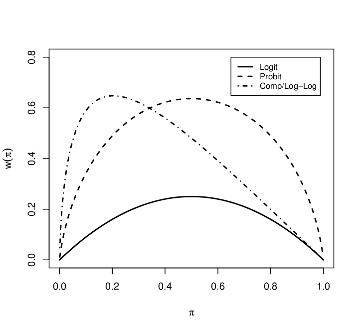
For a binary response, we consider the commonly used link functions including logit, probit, log-log and complimentary log-log links. Figure 1 illustrates the range of for specific link functions. The logit link corresponds to whereas for the probit link and for the (complementary) log-log links . It should also be noted that the -curve is symmetric for logit and probit links but asymmetric for the (complementary) log-log link. To examine the robustness for mis-specification of for different links, we assume for some constants and , since leads to trivial cases.
Fixing a chosen , let , . Without any loss of generality, we assume . It follows from Lemma 2.1 that . For the true , define with , . In practice, the experimenter might have some rough idea about the range of the parameter values and our next Theorem specifies the worst possible performance of a chosen design for that assumed range.
Theorem 4.1.
Suppose and , .
- (i)
If , then , where , and the maximum can only be attained at .
- (ii)
If , then can only be attained at , , or .
If can be as small as , for example, for logistic regression, , then the upper bound for will go to . As a direct conclusion from Theorem 4.1, we obtain
Corollary 4.1.
Suppose and , .
- (i)
If , then .
- (ii)
If , then .
To find out the most robust design in terms of maximum relative loss, we need explicit formulas of for case (ii) of Theorem 4.1. To simplify the notations, let , , , . Then . Let
Then and the in case (ii) of Theorem 4.1 is
Let and . Based on Corollary 2.1 and Corollary 2.2,
Note that is actually a function of .
Theorem 4.2.
Suppose , , . Then attains its minimum if and only if , which is the uniform design.
In other words, the uniform design is the most robust one in terms of the maximum of relative loss of efficiency. Note that the conclusion of Theorem 4.2 is still true even if is replaced with .
4.2 Simulation study
To study the robustness measured by percentiles of other than the maximum , we randomly select 1000 vectors , . For the logit link, . If we randomly select ’s between and , the chance of getting a saturated design can be as high as 48% when some is close to and the condition of Theorem 2.1 applies. We try to skip the cases that give a saturated design since in those cases both the exact solution and robustness are clearly known. So here we consider only. Then the chance of saturated design drops to 6% for uniformly distributed ’s. So, for the logit link, we consider and for the other links, .
Suppose is the true , and is the chosen (assumed) . We consider 1000 cases. In our robustness study, each one of the 1000 ’s is chosen in turn as and the remaining 999 cases are regarded as respectively. We use CAD to determine the optimal designs and corresponding to and , respectively.
 |
 |
For the numerical computations in this section, we consider the upper 99th percentile of and denote it by . This corresponds to the worst case scenario. The left panel of Figure 2 illustrates that this relative loss will range roughly between 0.1 and 0.4, whereas the right panel helps us identify those ’s with non-robust optimal solution . The horizontal axis corresponds to the distance between and divided by , where . The vertical axis is our robustness measurement . There is a clearly positive association between the relative loss and the distance. We have examined the other quantiles such as the 25th quantile, median, 75th quantile, and 95th quantile of . The patterns are similar for all of them. From this, we conclude that the locally -optimal designs are quite robust and the farther the ’s are from the saturation condition (2), the smaller is the relative loss of efficiency. It is interesting to note that the left most point (denoted by ) on the right panel of Figure 2 corresponds to the uniform design. It can be verified that the standardized distance attains its minimum if and only if which leads to the uniform design. While the left panel of Figure 2 indicates that the performance of the “worst 1%” designs is not too bad in terms of robustness, the right panel (as well as figures of other quantiles, not shown here) clearly demonstrates the significance of the saturation condition. The points with values greater than 0.15 either satisfy or almost satisfy the saturation condition. This figure also suggests that the uniform design is highly robust.
Similar results have been obtained for probit and (complementary) log-log links.
5 Robustness of Uniform Design
If the experimenter is unable to make an informed choice of the assumed values for local optimality, the natural design choice is the uniform design The relative loss of efficiency of with respect to the true is:
It can be shown that
where , is the optimal design under , and is defined in (1).
5.1 Maximum relative loss of uniform design
We denote by the maximum loss of efficiency of the uniform design. The following theorem formulates with different values of ’s and generalizes Theorem 4.1.5 of Mandal, Yang and Majumdar (2010).
Theorem 5.1.
Suppose , . Let . Then
where , and is the 3rd root of the equation

Figure 3 reveals the nature of association between the maximum relative loss of uniform design and the ratio between the upper and lower limits of range of ’s. It can be seen that if the performance of uniform design become worst when is 10 or more, but even in that case is less than 1/4. Note that the fact was established in Mandal, Yang and Majumdar (2010). Uniform design performs moderately well when lies between 3 and 10, and it performs extremely well if .
5.2 A real example
The data given in Table 1, reported by Collett (1991), were originally obtained from an experiment conducted at the East Malling Research Station (Hoblyn and Palmer, 1934). The experimenters investigated the vegetative reproduction of plum trees. Cuttings from the roots of older trees of the palms named Common Mussel were taken between October, 1931 and February, 1932. This experiment involved two factors each at two levels. The first factor was time of planting (root stocks were either planted as soon as possible after they were taken, or they were imbedded in sand under cover and were planted in the next spring). The second factor was the length of root cuttings (6 cm or 12 cm). Hoblyn and Palmer used an uniform design and a total of 240 cuttings were taken for each of the four combinations. The response was the condition of each plant (alive or dead) in October, 1932.
| Length of | Time of | Number of surviving |
|---|---|---|
| cutting | planting | out of 240 |
| Short | At once | 107 |
| In Spring | 31 | |
| Long | At once | 156 |
| In Spring | 84 |
After fitting the logit model, we get, and the corresponding . If we use this , the optimal proportions are . The corresponding determinant of is . On the other hand, the determinant of the information matrix corresponding to the uniform design is . Thus the uniform design is 99.1% efficient. If this was the first of a series of experiments, then the result supports the continued use of the uniform design. Similar calculations with the probit link shows that the uniform design is 99.9% efficient.
6 Discussion
In this paper and our earlier work, Mandal, Yang and Majumdar (2010), we have investigated various aspects of locally -optimal designs for experiments with binary response. Extending these results to experiments with more than two factors is far from a straightforward task. The main difficulty is that a concise expression like is not available. We are currently investigating different methods for the general case. For some special cases, however, the results can be derived with relative ease. For instance, for the fraction of given by it can be shown that the uniform design is locally -optimal no matter what the assumed values of the parameter may be.
Appendix
1. Proof of Theorem 4.1
To simplify the notations, we use instead of here. Note that for any . Suppose , . To minimize , we only need to consider those cases with .
If , then and . Thus and . Fixing , it can be verified that
where “" is true if and only if . In this case,
where . Note that in this case.
Suppose . Then and . Again, we fix and assume , .
Case 1: If , and then , where “" is attained if and only if and . In this case, .
Case 2: If and , then .
Actually, in this case, . It can be verified that for small enough ,
where , and .
From now on, we only need to consider with and . In this case, .
Similarly, it can be verified that
(1) If , then
.
(2) If , then
.
(3) If , then
.
(4) If , then
.
In summary, if , then
Based on the proof, the minimum of can only be obtained at , , or .
2. Proof of Theorem 4.2
Given and , it can be verified that
where the second “" is true if and only if . Similarly, where “" is true if and only if ; where “" is true if and only if . Therefore, if ,
attains its maximum only at . In other words, the uniform design has smaller than any other design with .
On the other hand, it can be verified that if , the maximum relative loss of uniform
for any design with .
In short, attains its minimum only at the uniform design.
3. Proof of Theorem 5.1
Let (or ) and . Then
Since , it can be verified that and the “" is true if and only if , that is, . Thus .
Now we only need to compare with . It can be verified that
- (i)
If , or , .
- (ii)
If , .
- (iii)
If , then .
Here is the 3rd root of equation
Then can be obtained accordingly.
References
- Agresti (2003) Agresti, A. (2003). Categorical Data Analysis, John Wiley, New York.
- Collett (1991) Collett, D. (1991). Modelling Binary Data, Chapman & Hall/CRC, New York.
- Fotiou, Parrilo and Morari (2005) Fotiou, I. A., Parrilo, P. A., and Morari, M. (2005). Nonlinear parametric optimization using cylindrical algebraic decomposition. In Proceedings of the 44th IEEE Conference on Decision and Control, and the European Control Conference 2005, 37353740.
- Hoblyn and Palmer (1934) Hoblyn, T. N. and Palmer, R. C. (1934). A complex experiment in the propagation of plum rootstocks from root cuttings: season, 19311932, Journal of Pomology and Horticultural Sciences, 12, 3656.
- Karush (1939) Karush, W. (1939). Minima of functions of several variables with inequalities as side constraints. M.Sc. Dissertation. Dept. of Mathematics, Univ. of Chicago, Chicago, Illinois.
- Khuri, Mukherjee, Sinha and Ghosh (2006) Khuri, A. I., Mukherjee, B., Sinha, B. K. and Ghosh, M. (2006). Design Issues for Generalized Linear Models: A Review. Statistical Science, 21, 376399.
- Kuhn and Tucker (1951) Kuhn, H. W. and Tucker, A. W. (1951). Nonlinear programming. Proceedings of 2nd Berkeley Symposium, Berkeley: University of California Press, 481492.
- Mandal, Yang and Majumdar (2010) Mandal, A., Yang, J. and Majumdar, D. (2010). Optimal designs for two-level factorial experiments. University of Georgia Technical Report, Stat 2010-4.
- McCullagh and Nelder (1989) McCullagh, P. and Nelder, J. (1989). Generalized Linear Models, Second Edition, Chapman and Hall/CRC, Boca Raton.
- Nocedal and Wright (1999) Nocedal, J. and Wright, S. J. (1999).Numerical Optimization, Springer, New York.