Counting Connected Set Partitions of Graphs
Abstract
Let be a simple undirected graph with vertices then a set partition of the vertex set of is a connected set partition if each subgraph induced by the blocks of is connected for . Define as the number of connected set partitions in with blocks. The partition polynomial is then . This paper presents a splitting approach to the partition polynomial on a separating vertex set in and summarizes some properties of the bond lattice. Furthermore the bivariate partition polynomial is briefly discussed, where counts the number of connected set partitions with blocks and intra block edges. Finally the complexity for the bivariate partition polynomial is proven to be -hard.
The authors Frank Simon and Martin Trinks receive a grant from the European Union.
![[Uncaptioned image]](1005.1726v2/esf_logo.png)
![[Uncaptioned image]](1005.1726v2/euemblem_eps.png)
Keywords: graph theory, bond lattice, chromatic polynomial, splitting formula, bounded treewidth, -hard
1 Introduction
One of the best-studied graph polynomials is the chromatic polynomial , giving the number of proper vertex colorings of an undirected graph with at most colors (see e.g. [2, 8, 9, 12, 11]). Rota [3] showed that the chromatic polynomial of a graph is uniquely defined by its bond lattice . The bond lattice can be defined as a sublattice of the partition lattice on . A set partition belongs to iff all blocks of induce connected subgraphs of .
We investigate here the rank-generating function of , which we call the partition polynomial . There are two ways to consider , namely from an order-theoretic point of view (as rank-generating function) or as a graph polynomial. We pursue here the second way. The first natural question in this context is: Does the partition polynomial determine the chromatic polynomial ? We will show that this is not the case. Even the converse statement is false. There are pairs of non-isomorphic graphs with coinciding chromatic polynomials but different partition polynomials. The next interesting problem is the derivation of graph properties and graph invariants from the partition polynomial. Which graphs are uniquely determined by their partition polynomials? We call non-isomorphic graphs with coinciding partition polynomial partition-equivalent. Can we characterize partition-equivalent graphs?
The computation of the partition polynomial is the next challenge. The obvious way, to list all connected vertex partitions (partitions of ) and count them with respect to the number of blocks is even for small graphs often too laborious. Consequently, each method that simplifies the computation of the partition polynomial is welcome.
Thus, the next task is the identification of graph classes permitting a polynomial-time computation of the partition polynomial. Let be a graph and and edge-disjoint subgraphs of that have a vertex set in common. Then a splitting formula permits to find by separate computation of certain polynomials assigned to and . The here presented splitting formula for the partition polynomial is the first step to find a polynomial time algorithm for graphs of bounded treewidth.
Edges linking different blocks of a connected set partition form a cut set. An edge cut of corresponds to a cut set defined by a connected two-block partition. In order to keep track of the number of edges forming a cut set, we extend the partition polynomial into a bivariate polynomial.
The paper is organized as follows. Section 2 provides a short introduction into set partitions and their order properties. Connected set partitions of the vertex set of a given graph are introduced in Section 3. The main object of this paper, the partition polynomial , is defined in Section 4. This section provides also basic properties of the partition polynomial, some graph invariants that can be derived from , recurrence formulae, and results for special graphs. Section 5 deals with one of the main results of the paper - the splitting formula for the partition polynomial. The last section presents the two-variable extension of the partition polynomial and some examples of non-isomorphic partition-equivalent graphs as well as pairs of graphs that are chromatically equivalent and not partition-equivalent and vice versa.
Finally, we can show that the computation of the extended partition polynomial is #P-hard, whereas complexity results for the simple partition polynomial are still not known.
2 Set partitions
A set partition of a finite set is a set of mutually disjoint and nonempty subsets , the blocks of , so that the union of the is . The number of blocks of a set partition is denoted by and the set of all set partitions of by . The number of set partitions of an -element set with exactly blocks is called the Stirling number of the second kind, which is denoted by . The Bell number is the number of all set partitions of an -element set, hence . Note that and equals , as there is exactly one set partition of the empty set with no blocks, namely .
Let and set if every block of is a subset of a block in , then becomes a poset. The maximal element of this poset is the set partition that has only one block and the minimal element is the set partition that consists only of singleton blocks. This poset is even more a lattice, i.e. for every two partitions there exists a smallest upper bound and a greatest lower bound in .
Assume that is a subset of , then induces the set partition in by setting , so that only the nonempty blocks are taken over to . The notation is used to indicate that induces in .
Let be finite sets and , set partitions of and , respectively. Then denotes the smallest upper bound of the set partitions and , where consists of the blocks and the remaining blocks being singletons and consists of the blocks and the remaining blocks being singletons.
3 Connected set partitions
A simple undirected graph or short graph is a pair consisting of a finite set , the vertices, and a subset , the edges, of the two element subsets of . If is a vertex subset of , then denotes the subgraph induced by that has the vertex set and all edges of that have both end vertices and in .
Let then is a connected set partition in if for all the subgraphs induced by are connected. The set of all connected set partitions in a graph is denoted by .
Consider the graph depicted in Figure 1, that has 89 distinct connected set partitions,
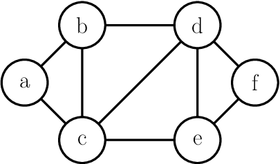
two of them are and . For the complete graph with vertices it is .
There is a constructive way to generate all connected set partitions of a given graph . In preparation of this construction assume that the vertices of the graph are considered as the one element sets . Let , then is the graph obtained from by contraction of the edge . If an edge is contracted the vertex obtained by merging the two vertices and is denoted by and is the union of the vertex subsets and of the original graph. As a result of any sequence of edge contractions of , the graph is obtained, where forms a connected set partition of . The set of all connected set partitions that can be obtained by such edge contractions of is again . Hence is sometimes called the lattice of contractions.
Another interpretation of the set of connected set partitions of a graph is given by the following procedure. Denote by the set partition of the vertex set induced by the connected components of the graph , hence iff is connected. Let with be a subgraph of . The components of then induce a set partition . Two vertices are elements of the same block of iff these vertices belong to the same component of . Observe that a set partition belongs to iff there is an edge subset and a spanning subgraph such that holds.
Lemma 1.
Let be a forest with edges. Then .
Proof.
Each edge subset of the forest generates a connected set partition . Conversely, if then there exists a subset with . Assume there is a different edge set with . In this case there are components and of and , respectively with the same vertex set but different edge sets. Consequently, contains a cycle which contradicts the premise that is a forest. Hence each edge subset induces a unique set partition of . ∎
Further properties of the set are easy to verify:
- 1.
If then .
- 2.
is a geometric lattice, i.e. each element of is the smallest upper bound of some elements covering . These connected set partitions consist of one block with exactly two elements and otherwise only singleton blocks. Hence every two element block of such an atomic connected set partition can be identified with an edge of .
The lattice of connected set partitions also occurs under the name bond lattice or lattice of contractions in the literature [7].
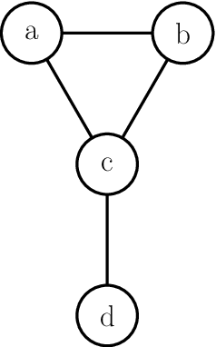

Figure 2 shows a graph with vertex set . Figure 3 represents the lattice of connected set partitions of this graph.
A vertex coloring of is a function from the set of vertices of to a finite set of colors . A vertex coloring is proper if implies . Denote by the chromatic polynomial of , i.e. the number of proper vertex colorings of using a color set with exactly colors. For let be a set of colors. For let be the number of vertex colorings of with colors of such that all vertices that belong to one block of are colored alike and such that end vertices of an edge that link different blocks of are colored differently. Let the graph obtained from by merging all vertices that are contained in one and the same block of . Then we see that the function can be represented as a chromatic polynomial by . For each coloring there exists a unique such that contributes to . The number of all colorings with at most colors that assign the same color to all vertices of a block of is . Let , then it is
and by Möbius inversion the equation
is obtained. The chromatic polynomial of corresponds to , which gives Theorem 2 presented in [3].
Theorem 2 (Rota).
The chromatic polynomial of a graph satisfies
4 The partition polynomial
The notion of connected set partitions of a graph is utilized to define the partition polynomial
| (1) |
where the coefficients count the number of connected set partitions of with blocks, e.g. consider the example graph depicted in Figure 1, page 1 then it is
Define to be the null graph. It is , which corresponds to the only connected set partition of the null graph - the empty set partition , that has no blocks at all. For no graph other than the null graph, the empty set partition is an element of , which gives . For the empty graph (edgeless graph) with vertices the partition polynomial is obtained. The only connected set partition in is . The set partition is a connected set partition for any graph. Hence the partition polynomial has degree . The greatest set partition , consisting of one block, namely itself, is connected iff is connected. Thus it is
More generally, the minimal degree of the partition polynomial (the least appearing power in ) equals the number of components of .
In the complete graph with vertices, each set partition of the vertex set is a connected set partition, which implies
A connected set partition of with exactly blocks consists of one pair (two-element set) and singletons (one-element sets). The pair corresponds to an edge of . Consequently, is obtained. A cutset in a graph is a subset , such that has more components than , but no proper subset of has this property. If is connected then equals the number of cutsets of .
Lemma 3.
Let be a graph with vertices and edges. Then the coefficient of the partition polynomial of satisfies
Proof.
A connected set partition of with blocks can have two different
types:
(1) Set partitions consisting of two vertex pairs and singletons
else.
(2) Set partitions with one tri-element block and singletons.
Each set partition of the first type corresponds to a unique selection of two
non-adjacent edges of . A selection of two edges that have one vertex in
common generates a set partition of the second type. However, if the three
vertices of the block induce a triangle in then there exist two other
selections of two edges generating the same connected block. The subtraction
of twice the number of triangles of in the given formula takes this fact
into account.
∎
In a similar way the following equation for a triangle-free graph with edges is proven:
As a more general conclusion the following statement is obtained.
Let be a graph with edges and its partition polynomial. If for the relations and are satisfied then the girth of equals . The number of cycles of length is in this case
Dowling and Wilson [10] proved a theorem on Whitney numbers of the second kind in geometric lattices that translates directly into an inequality for the coefficients of the partition polynomial.
Theorem 4 (Dowling and Wilson).
The coefficients of the partition polynomial satisfy for any connected graph with vertices and for each the inequality
Lemma 5.
If is a bridge of then
Proof.
Let be a bridge of . Each connected set partition of belongs to one of two classes:
(1) Set partitions that contain a block
with and .
(2) Set partitions for which and
belong to different blocks.
Each set partition of the first class
corresponds to a connected set partition of that is obtained by replacing
and by a single vertex. The set partitions of the second class are exactly the set partitions of .
∎
Corollary 6.
Let be a graph and its partition polynomial. If is a vertex of degree 1, then
Corollary 6 can be applied to compute the partition polynomial of a tree with vertices; the result is
The following decomposition formula is the basis in order to derive the partition polynomial of an arbitrarily given graph. Let be a graph and a vertex subset, then denotes the graph obtained from by removing all vertices of .
Theorem 7.
Let be a graph and , then
Here the sum is taken over all vertex induced connected subgraphs that contain .
Proof.
Let be a given vertex of . For each connected set partition with the induced subgraph is connected and is a connected set partition of . All connected set partitions that include are counted by . The blocks of a connected set partition can always be renumbered in such a way that is valid. Consequently, is the ordinary generating function for the number of connected set partitions of that have a block containing . Choosing the block containing in every possible way (such that the induced subgraph is connected) gives the desired result. ∎
The application of Theorem 7 to the partition polynomial of a cycle yields
The application of Theorem 7 requires the summation over all connected subgraphs containing , which results in an exponentially increasing computational effort. The following recursion includes only the neighborhood of a vertex. However, in this case, we need the principle of inclusion and exclusion.
Theorem 8.
For each subset let be the graph obtained from by merging all vertices of into a single vertex. Possibly arising parallel edges are replaced by single edges. Then the following equation is valid for each vertex :
Proof.
The first term on the right hand side of the equation counts all connected set partitions of that contain the singleton . All remaining connected set partitions of have the property that and at least one neighbor vertex of are together in a block. Let , then is the ordinary generating function for the number of connected set partitions of containing a block with . However, if analogously the connected set partitions of that have a block with are counted by with , , then all connected set partitions with a block containing are counted twice. Hence it is necessary to subtract . By induction on the number of vertices in the inclusion-exclusion representation as stated in the theorem is obtained. ∎
Theorem 9.
For an edge subset let the graph obtained from by contracting all edges of in . If is a cut of , then
| (2) |
holds.
Proof.
Let be a subset of the given cut and let be the number of connected set partitions of with exactly blocks such that the end vertices of any edge of are contained completely in one block. We define the polynomial
If is an edge of then the polynomials and coincide, since in both cases we count only connected set partitions of having and in one block. The generalization of this statement yields
for all . Let be the number of connected set partitions with such that the end vertices of any edge of are contained completely in one block and such that no two end vertices of any edge of belong to one and the same block of . We consider the generating function for these number sequence, i.e.
For any subset , we conclude
which yields via Möbius inversion
The polynomial counts all connected set partitions of that have no edge of as a subset of a block. Hence each block of a set partition counted by is completely contained in one component of , which gives
It is possible to state the partition polynomial of the complete bipartite graph in a closed form by the following theorem.
Theorem 10.
The partition polynomial of the complete bipartite graph is
| (3) |
Proof.
Assume the vertex set of the complete bipartite graph is such that and and each edge of links a vertex of with a vertex of . First we select a vertex subset , of size and a vertex subset , of size . There are possibilities for this selection. These vertices form singletons of the connected partition. The remaining vertices of are partitioned into blocks. A second partition with blocks is generated out of . These partitions are counted by the Stirling numbers of the second kind, more precise by the product . We form a bipartite graph with exactly components and without isolated vertices with the vertex set . The vertex set of one component of the bipartite graph consists of one block of a partition of and one block of a partition of . These blocks can be assigned to each other in different ways. The number of blocks of the resulting connected partition of is , which is taken into account by the power of . The triple sum counts all possible distributions of subsets and partitions. ∎
Corollary 11.
The complete bipartite graph and satisfy, respectively,
In order to state the Theorem 12 it is necessary to introduce the notion of the extraction of an edge from a given graph , as done in [1]. Assume that , then denotes the graph that emerges from by removing the edge and the two endvertices and from . This extraction of edges is easily generalized to arbitrary matchings of by successively extracting all matching edges in from .
Theorem 12.
Let be a graph and a matching in , so that every matching edge has the property that and are connected to every other vertex in . Then
| (4) |
holds.
Proof.
Let and denote by the set of all connected set partitions of containing the two element block . Then one has by virtue of the inclusion-exclusion principle
| (5) |
where the universal set is given by the set of all connected set partitions in .
For the right hand side note that the generating function of the connected set partitions in is given by , as the pairwise disjoint two element blocks created by the matching edges are yielding extra blocks, whereas accounts for the removal of these two element blocks.
For the left hand side one has to show that iff is a connected set partition in .
Let and a block of . Firstly, assume that and are distinct vertices in that are not both endpoints of an matching edge in . As induces a connected subgraph in , there is an - path in , that possibly uses edges of . Assume that this path is given by with and . Let be the possible first matching edge in , then one can shortcut the - path to , as the endpoints of every matching edge are connected to every other vertex in . Furthermore note that the edge cannot be a matching edge, as and would be incident. Hence and are also connected in the subgraph induced by in .
Secondly, assume that and are distinct vertices in that are endpoints of an matching edge in . By assumption there must be a third vertex distinct from and , so that the non matching edges and exist. Hence is an - path in the subgraph induced by in .
Therefore the removal of the edges in will not destroy the connectivity of and is also a connected set partition in .
Conversely suppose that is a connected set partition in , then will not contain any block corresponding to matching edges in and adding the edges in cannot destroy the connectivity of the blocks of , so that is also a connected set partition in .
By considering the generating function of the set of connected set partitions of the result for the left hand side follows. ∎
An application of Theorem 12 is given by the Corollary 13, where by the symmetry of the some simplifications are possible.
Corollary 13.
Let be a matching with exactly edges of the complete graph . Then
| (6) |
5 The splitting formula
The aim of this section is to derive a more general computational device to compute the partition polynomial of an arbitrarily given graph . The splitting formula on a separating vertex set presented in this section can be employed to construct an algorithm with polynomial running time that computes the partition polynomial for graphs with bounded treewidth.
Given a graph and subgraphs , of G, so that , and , is satisfied, then is a splitting of . The set is a separating vertex set of .
Let , then for denotes the set of connected set partitions of , that are inducing in . Let be the graph emerging from by adding edges between all vertices of in , so that becomes the complete graph on the vertex set .
If , then induces the connected set partition
in by the connected components of the subgraphs induced by the blocks . It is iff is a connected set partition of . Note that this definition also implies the inequality for all . Consider the set partition and the graph depicted in Figure 1 on page 1 then as shown in Figure 4.

Note that the block splits into the blocks and , as the former block does not induce a connected subgraph in the underlying graph .
Let be a graph, and , then is defined as the set
| (7) |
and the associated counting polynomial as
| (8) |
Observe that if not holds one has and therefore also . Furthermore note that in the case of it is
It is notable that the connected set partitions of a graph can be partitioned into disjoint sets by considering the set partitions that they are inducing in . Therefore the polynomials can be used to determine the partition polynomial by the sum
| (9) |
The central Lemma 14 shows how a connected set partition in is assembled, given a splitting of and the connected set partitions in the subgraphs and .
Lemma 14.
Let be a graph and a splitting of .
Let and , , respectively. Then and holds, satisfying and .
Conversely let and , then satisfying .
Proof.
Let with and . Consider a block , then the construction of can be distinguished in the case (a) and the case (b) , as been exemplified in Figure 5.
Note that , are connected, possibly empty, subgraphs of , , for the given block , by considering the distinct cases and . Even more observe that holds, so that and is satisfied.
In the case (a) it is . Set and . As is a separating vertex set of either and or and can occur, as being exemplified in Figure 5 by the blocks and . Hence the conditions and are satisfied.
In the case (b) it is , so that , and holds with , as is a separating vertex set of and as induces in . Note that is satisfied. An example for this case is found in Figure 5 through the block , which is the union of the blocks and . Even more the relation holds. This case is exemplified in Figure 6 through , and, .
For all the conditions and hold with and . Recalling that a block can either decompose into one block (a) in or or two blocks (b) in and , as is a separating vertex set, the desired claim with and follows.
Note that the set partition is a connected set partition in with , by considering the cases (a) and (b), depicted in Figure 5.
In the case (a) it is assumed without loss of generality that holds with and . It is then and even more , where is set.
In the case (b) let and be the blocks, so that holds and set , then is satisfied and even more is true as being exemplified in Figure 6.
The application of the above argumentation to all blocks of yields the proof of the converse claim. ∎

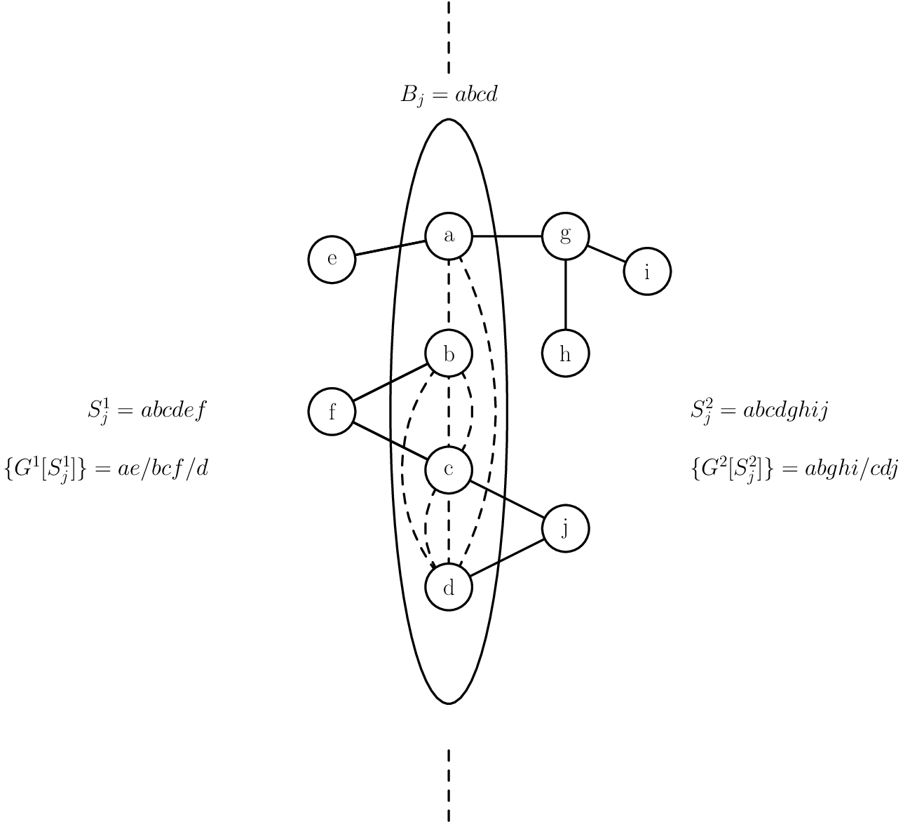
Lemma 14 is then utilized to deduce Theorem 15, that allows the computation of by considering the subgraphs and of a splitting .
Theorem 15.
Let be a graph, a splitting of and . Then
| (10) |
Proof.
Due to Lemma 14 every two connected set partitions , in the subgraphs , inducing in , constitute a connected set partition in that induces in satisfying , and even more every connected set partition of inducing in emerges in this way.
Setting , and yields under the view of the condition .
Therefore the product counts the number of connected set partitions in that are inducing in satisfying , and, . However there is an overcounting done by simply taking the product, as every block of the connected set partition of that has a nonempty intersection with is counted twice by both factors of the product, which complies with the case (b) in the proof of Lemma 14. Therefore it is necessary to divide the product by the factor , as there are exactly blocks with this property. The summation ranges over all and with , as only the connected set partitions with are counted by . ∎
Finally the announced splitting formula is deduced by application of Theorem 15 and the Equation (9).
Theorem 16.
Let be a graph and a splitting of . Then
| (11) |
The computational requirements of Theorem 16 can be reduced, if the intersection of the subgraphs and is the complete graph of the separating vertex set . In this case the polynomials and will vanish for all with .
Corollary 17.
Let be a graph and a splitting, so that holds. Then
| (12) |
Corollary 17 covers two special cases, that exhibit a special simple form, namely and . As in the case of two disjoint graphs and it is
and in the case of an articulation
Observe that the above two formulas also occur in the computation of the chromatic polynomial of the graph , e.g.
| (13) |
and
| (14) |
are valid as well.
6 Clusterings in graphs
This brief section presents a possible generalization of the partition polynomial, the minimal cut polynomial. Most formulas derived in the previous sections are readily transfered to this more general polynomial.
Let be a graph and a connected set partition. Denote by the edge set of the subgraph induced by for all . Then
denotes the set of intra block edges, where is a connected set partition in .
Let be a graph with vertices and edges. The bivariate minimal cut polynomial is an extension of the partition polynomial that accounts for the edges by introducing the counting variable :
| (15) | ||||
| (16) |
The coefficients can be interpreted as the number of connected set partitions of with blocks and edges, whose endvertices belong to the same block or as the number of clusterings in with blocks and intra-cluster edges. Note that , so that the minimal cut polynomial is an extension of the partition polynomial.
The minimal cut polynomial of the graph depicted in Figure 1 is
In analogy to Corollary 6, vertices with degree one can be reduced.
Corollary 18.
Let be a graph and the minimal cut polynomial of . If is a vertex of degree 1, then
Let be an arbitrary tree with vertices, then Corollary 18 can be applied times, hence
In the same vein Theorem 7 generalizes to the minimal cut polynomial.
Theorem 19.
Let be a graph and , then
The application of Theorem 19 to the cycle of length yields
Similarly Theorem 19 can be applied to the complete graph on vertices, yielding the recurrence relation
with the initial condition .
It is notable that the exponential generating function of the sequence
is conveyed by application of the exponential formula [5]
so that the sum representation
is found, where the sum ranges over all partitions of the number , where the number of parts of size is given by , hence holds.
Theorem 16 is also easily transfered to the minimal cut polynomial, where the are defined in analogy to the . Note that by the definition of the splitting no overcounting of edges occurs that has to be considered, as with holds, for every splitting of .
Theorem 20.
Let be a graph and a splitting of . Then
In the special cases and again
and
is satisfied.
7 Distinctive power
Two graphs and with coinciding partition polynomials are said to be partition equivalent and likewise chromatically equivalent, if their chromatic polynomials coincide. In the view of Theorem 2 it is remarkable that there are graphs that are partition equivalent, but not chromatically equivalent and conversely that there are graphs, which are chromatically equivalent, but not partition equivalent.

Consider for example the graphs and depicted in Figure 7 that are chromatically equivalent
but with the distinct partition polynomials

and observe that the graphs and depicted in Figure 8 are partition equivalent
with the distinct chromatic polynomials
The efficient construction of graphs that are partition equivalent, but not chromatically equivalent remains an open problem. The smallest counterexample depicted in Figure 8 was found after an exhaustive computer search using a library of nonisomorphic graphs found in [6].
8 Complexity
Theorem 21.
The computation of the two-variable polynomial is #P-hard.
Proof.
Goldschmidt and Hochbaum [4] show that the -cut problem is NP-complete by reducing it to the maximum clique problem. The -cut problem defined as follows: Given an undirected graph and a number , find a minimum edge subset (a -cut) that, when deleted, separates the graph into exactly components. Assume we know the partition polynomial . Then the coefficient is the number of edge subsets such the graph has exactly components. Consequently, the smallest power of in yields the minimum number of edges that form a -cut of . ∎
References
- [1] Ilya Averbouch, Johann A. Makowsky, and Peter Tittmann. A graph polynomial arising from community structure (extended abstract). In WG, pages 33–43, 2009.
- [2] C.D. Birkhoff and D.C. Lewis. Chromatic polynomials. Trans. Amer. Math. Soc., 60:335–351, 1946.
- [3] G. Rota. On the Foundations of Combinatorial Theory: I. Theory of Möbius Inversion. Z. Wahrscheinlichkeitstheorie 2, pages 340–368, 1964.
- [4] Olivier Goldschmidt and Dorit S. Hochbaum. A polynomial algorithm for the k-cut problem for fixed k. Mathematics of Operations Research, 19(1):24–37, 1994.
- [5] H. S. Wilf. generatingfunctionology. Academic Press, 1990.
- [6] B. D. Mc Kay. Combinatorial data. Private homepage, Sep 2009. http://cs.anu.edu.au/~bdm/data/graphs.html.
- [7] R. P. Stanley. A Symmetric Function Generalization of the Chromatic Polynomial of a Graph. Advances in Mathematics, 111(1):166–194, 1995.
- [8] R.C. Read. An introduction to chromatic polynomials. J. Combin. Theory, 4:52–71, 1968.
- [9] R. P. Stanley. Acyclic orientations of graphs. Discrete Mathematics, 5:171–178, 1973.
- [10] T. A. Dowling and R. M. Wilson. Whitney Number Inequalities for Geometric Lattices. Proceedings of the American Mathematical Society, 47:504–512, Feb 1975.
- [11] W. T. Tutte. Chromials. Springer Lecture Notes in Mathematics, 411:243–266, 1974.
- [12] W.T. Tutte. On chromatic polynomials and the golden ratio. J. Combin. Theory, 9:289–296, 1970.