Singular perturbation of polynomial potentials with applications to -symmetric familiesThanks: A. Eremenko was supported by NSF grant DMS–0555279, and by the Humboldt Foundation; A. Gabrielov was supported by NSF grant DMS–0801050.
Abstract.
We discuss eigenvalue problems of the form with complex polynomial potential , where is a parameter, with zero boundary conditions at infinity on two rays in the complex plane. In the first part of the paper we give sufficient conditions for continuity of the spectrum at . In the second part we apply these results to the study of topology and geometry of the real spectral loci of -symmetric families with of degree and , and prove several related results on the location of zeros of their eigenfunctions.
MSC: 34M35, 35J10. Keywords: singular perturbation, one-dimensional Schrödinger operators, eigenvalue, spectral determinant, -symmetry.
1. Introduction
We consider eigenvalue problems
| (1.1) |
Here is a polynomial in the independent variable , which depends on a parameter , and are two rays in the complex plane. The set of all pairs such that is an eigenvalue of (1.1) is called the spectral locus.
Such eigenvalue problems were considered for the first time in full generality by Sibuya [40] and Bakken [2]. Sibuya proved that under certain conditions on and the leading coefficient of , there exists an infinite sequence of eigenvalues tending to infinity. If
| (1.2) |
where then the spectral locus, which is the set of all such that is an eigenvalue of 1.1, is described by an equation Here is an entire function of variables, called the spectral determinant. So the spectral locus of (1.1), (1.2) is an analytic hypersurface in . It is smooth [2] and connected for [1, 30].
In the first part of this paper we study what happens to the eigenvalues and eigenfunctions when the leading coefficient of tends to zero.
Bender and Wu [8] studied the quartic oscillator as a perturbation of the harmonic oscillator:
| (1.3) |
Here and in what follows means that the boundary conditions are imposed on the positive and negative rays of the real line. It has been known for long time that the eigenvalues of (1.3) converge as to the eigenvalues of the same problem with , but they are not analytic functions of at (perturbation series diverge). To investigate this phenomenon, Bender and Wu considered complex values of and studied the analytic continuation of the eigenvalues as functions of in the complex plane. Their main findings can be stated as follows: the spectral locus of the problem (1.3) consists of exactly two connected components; for , the only singularities of eigenvalues as functions of are algebraic branch points. These statements were rigorously proved in [19]. Discoveries of Bender and Wu generated large literature in physics and mathematics. For a comprehensive exposition of the early rigorous results we refer to [41].
To perform analytic continuation of eigenvalues of (1.3) and similar problems for complex parameters, one has to rotate the normalization rays where the boundary conditions are imposed. One of the early papers in the physics literature that emphasized this point was [7]. Thus physicists were led to problem (1.1), previously studied only for its intrinsic mathematical interest.
An interesting phenomenon was discovered by Bessis and Zinn-Justin. For the boundary value problem
they found by numerical computation that the spectrum is real. This is called the Bessis and Zinn-Justin conjecture (see, for example, historical remark in [5]). This conjecture was later proved by Dorey, Dunning and Tateo [15, 16] with a remarkable argument which they call the ODE-IM correspondence, see their survey [17]. Shin [37] extended this result to potentials
| (1.4) |
with .
These results and conjectures generated extensive research on the so-called -symmetric boundary value problems. -symmetry means a symmetry of the potential and of the boundary conditions with respect to the reflection in the imaginary line . stands for “parity and time reversal”.
It turns out that the spectral determinant of a -symmetric problem is a real entire function of , so the set of eigenvalues is invariant under complex conjugation. In contrast to Hermitian problems where the eigenvalues are always real, the eigenvalues of a -symmetric problem can be real for some values of parameters, but for other values of parameters some eigenvalues may be complex. So we can see the “level crossing” (collision of real eigenvalues) in real analytic families of -symmetric operators, the phenomenon which is impossible in the families of Hermitian differential operators with polynomial coefficients.
In this paper, we first consider the general problem (1.1) and the limit behavior of its eigenvalues and eigenfunctions when
| (1.5) |
with , as , while the coefficients of are restricted to a compact set and does not approach zero. Then we apply our general results to certain families of -symmetric potentials of degrees and , and prove some conjectures made by several authors on the basis of numerical evidence.
In particular, our results for the -symmetric cubic (1.4) imply that no eigenvalue can be analytically continued along the negative -axis, and the obstacle to this continuation is a branch point where eigenvalues collide.
Another result is the correspondence between the natural ordering of real eigenvalues of (1.4) for and the number of zeros of eigenfunctions that do not lie on the -symmetry axis, conjectured by Trinh in [44]. This correspondence is similar to that given by the Sturm–Liouville theory for Hermitian boundary value problems.
A different approach to counting zeros of eigenfunctions is proposed in [27], where the authors prove that for large enough, the -th eigenfunction has zeros in a certain explicitly described region in the complex plane.
The plan of the paper is the following. In Section 2 we prove a general theorem on the continuity of discrete spectrum at for potentials of the form (1.5), with boundary conditions on two given rays. Previously such problems were studied using the perturbation theory of linear operators in [26, 41, 11]. Our method is different, it is based on analytic theory of differential equations.
Verification of conditions of our general result in Section 2 is non-trivial, and we dedicate the entire Section 3 to this. The question is reduced to the study of Stokes complexes of binomial potentials , which is a problem of independent interest, so we include more detail than it is necessary for our applications. The Stokes complex is the union of curves, starting at the zeros of , on which , so they are vertical trajectories of a quadratic differential. Stokes complexes occur in many questions about asymptotic behavior of solutions of equations (1.1). Our study permits us to make conclusions on the behavior, as , of the Stokes complexes of potentials where and is a family of polynomials of degree with bounded coefficients. We mention here [35] where a topological classification of Stokes complexes for polynomials of degree is given.
In the rest of the paper we apply these results to problems with -symmetry. In Section 4, we consider the -symmetric cubic family (1.4) with real and . We prove that the intersection of the spectral locus with the real -plane consists of disjoint non-singular analytic curves , the fact previously known from numerical computation [14, 43, 31]. Moreover, we prove that the eigenfunctions corresponding to have exactly zeros outside the imaginary line. (They have infinitely many zeros on the imaginary line). Furthermore, using the result of Shin on reality of eigenvalues, we study the shape and relative location of these curves in the -plane and show that on both ends of , and that for , consists of graphs of two functions, that lie below the graphs of functions constituting .
This gives –analog of the familiar fact for Hermitian boundary value problems that “-th eigenfunction has real zeros”; in our case we count zeros belonging to a certain well-defined set in the complex plane. This result proves rigorously what can be seen in numerical computations of zeros of eigenfunctions by Bender, Boettcher and Savage [6].
The result of Section 4 also gives a contribution to a problem raised by Hellerstein and Rossi [9]: describe the differential equations
| (1.6) |
with polynomial coefficient which have a solution whose all zeros are real. For polynomials of degree , all such equations are parametrized by our curve , and equations having solutions with exactly non-real zeros are parametrized by .
The arguments in Section 4 use our parametrization of the spectral loci from [21, 19] combined with the singular perturbation results of Sections 2 and 3. These perturbation results allow us to degenerate the cubic potential to a quadratic one (harmonic oscillator) and to make topological conclusions based on the ordinary Sturm-Liouville theory.
Next we apply similar methods to two families of -symmetric quartics
| (1.7) |
and
| (1.8) | |||
| (1.9) |
where is an integer. The first family was considered in [3] and [12, 13]. We prove that the spectral locus in the real -space consists of infinitely many smooth analytic surfaces , each homeomorphic to a punctured disc, and that an eigenfunction corresponding to a point has exactly zeros which do not lie on the imaginary axis. We study the shape and position of these surfaces by degenerating the quartic potential to the previously studied -symmetric cubic oscillator.
The second quartic family (1.8-1.9) was introduced by Bender and Boettcher [4]. It is quasi-exactly solvable (QES) in the sense that for every integer in the potential, there are “elementary” eigenfunctions, each having zeros. The part of the spectral locus corresponding to these elementary eigenfunctions is a smooth connected curve in [19, 20]. In the end of Section 4 we study the intersection of this curve with the real -plane. Similarly to the case of the -symmetric cubic, this intersection consists of smooth analytic curves , and for the eigenfunction has exactly zeros that do not lie on the imaginary axis. For the part of over some ray consists of disjoint graphs of two functions, and we have the following ordering: and imply that . Moreover, the QES spectrum for consists of the smallest real eigenvalues.
The results of Section 4 permit us to answer the question of Hellerstein and Rossi stated above for polynomial potentials of degree 4: All equations (1.6) that possess a solution with non-real zeros are parametrized by our curves if the total number of zeros is , and by our surfaces if the total number of zeros is infinite.
Notation and conventions.
1. What we call Stokes lines is called by some authors “anti-Stokes lines” and vice versa. We follow terminology of Evgrafov and Fedoryuk [23, 24].
2. We prefer to replace by in -symmetric problems. Then potentials become real, and the difference between -symmetric and self-adjoint problems is that in -symmetric problems the complex conjugation interchanges the two boundary conditions, while in self-adjoint problems both boundary conditions remain fixed by the symmetry. The main advantage for us in this change of the variable is linguistic: we frequently refer to “non-real” zeros. The expression “non-real” excludes , while the expression “non-imaginary” does not.
We thank Kwang-Cheul Shin for his useful remarks and for sending us the text of his lecture [39] and Per Alexandersson for the plots of Stokes complexes he made for this paper.
2. Perturbation of eigenvalues and eigenfunctions
We begin with recalling some facts about boundary value problem (1.1) with potential (1.2). The separation rays are defined by
These rays divide the plane into open sectors which we call Stokes sectors. We enumerate them by residues modulo counterclockwise.
A solution of the differential equation (1.1) is called subdominant in if as , for all . For every , the space of solutions of the equation in (1.1) which are subdominant in is one-dimensional. If and are adjacent, that is then the corresponding subdominant solutions are linearly independent.
Let and be two non-adjacent Stokes sectors. We consider the boundary conditions
| (2.1) |
Such boundary value problem has an infinite set of eigenvalues tending to infinity. All eigenspaces are one-dimensional. These facts were proved by Sibuya [40] whose main tool were special solutions normalized on one ray, which we call Sibuya solutions. Precise definition is given below. Our first goal is to prove continuous dependence of Sibuya solutions on parameters.
We consider a family of polynomial potentials with parameters :
| (2.2) |
Let be a compact set which has a fundamental system of open simply connected neighborhoods, and such that for . This compact will be fixed in all our arguments, so our notation does not reflect dependence of the quantities introduced below on . Let be a ray in .
Suppose that for some and for all the following conditions hold:
a) There exists such that for all zeros of such that .
b) Whenever intersects a vertical trajectory of at a point , , the smallest angle between this trajectory and at the intersection point is at least .
c) is not a separating direction of .
One can easily show that b) implies c). Condition c) simply means that is neither a Stokes line for , nor a Stokes line for .
Condition a) implies that there is a branch of analytic on . Let be the corresponding branch of . We choose the original branch in such a way that
This is possible in view of condition c).
Let us say that is a Sibuya solution of
if
Here . Notice that a change of , results is multiplying the Sibuya solution by a factor that depends only on and but not on .
Theorem 2.1.
Under the conditions a), b), c) above, there exists a unique Sibuya solution. It is an analytic function of in a neighborhood of , continuous on for every compact .
Proof.
Let
where the integral is taken along This is an analytic function which maps onto a curve . Condition b) implies that is a graph of a function (intersects every vertical line at most once), the slope of is bounded, and maps bijectively some neighborhood of onto a neighborhood of .
Let be the inverse function to .
Setting we obtain the differential equation
where the primes stand for differentiation with respect to , and
This is equivalent to the integral equation
| (2.3) |
where the path of integration is the part of from to . The integral equation is solved by successive approximation. We set , and obtain
| (2.4) |
which we abbreviate as Setting and , we obtain
Here we used the fact that on the curve of integration because is a graph of a function. Now, if is large enough, we have
| (2.5) |
for all values of parameters . We state this as a lemma:
Lemma 2.2.
There exists such that for the piece of from to and for all we have
The integral in this lemma equals to the integral in (2.5) by the change of the variable .
Proof. Let be all zeros of listed with multiplicity, in an order of non-decreasing moduli. Suppose that are in the disc while the rest are outside. Here is the number from condition a). We have
and
First we estimate
| (2.6) |
To estimate we first use condition a) to conclude that
| (2.7) |
where depends only on . Then
| (2.8) |
Applying these inequalities, we obtain that
on , where depends only on .
Now we write
Here we used inequality (2.7) with interchanged and . It is easy to see by Vieta’s theorem that
where depends only on . This shows that
Now we use the fact that is a part of a ray from the origin, so on Putting all this together we conclude that our integral is majorized by the integral
which proves the lemma.
So the series is convergent uniformly in for some and this convergence is uniform with respect to Then an application of the theorem on uniqueness and continuous dependence of initial conditions for linear differential equations shows that this convergence is uniform also on compacts in the right half-plane of the -plane. ∎
Let be a family of discrete subsets of the complex plane, depending on a parameter . We say that depends continuously on if there exists a family of entire functions such that is the set of zeros of , and depends continuously on . Here the topology on the set of entire functions is the usual topology of uniform convergence on compact subset of the complex plane.
Consider the eigenvalue problem
| (2.9) |
where is a polynomial in of the form (2.2), and are two rays from the origin in the complex plane. We say that a ray is admissible if conditions a), b) and c) in the beginning of this section are satisfied. The notion of admissibility depends on the parameter region participating in conditions a), b) and c).
Theorem 2.3.
If both rays and are admissible then the spectrum of problem (2.9) is continuous for .
Proof.
The limit problem (2.9) for may have no eigenvalues, this is the case when the rays and belong to adjacent sectors of . In this case, Theorem 2.3 says that the eigenvalues escape to infinity as .
Theorem 2.4.
Consider the problem (2.9), and suppose that the rays and are admissible, is an eigenvalue that depends continuously on and has a finite limit as . Then there exists an eigenfunction of this problem, corresponding to this eigenvalue, that depends continuously on .
Proof.
Let be the Sibuya solution of (2.9) with , corresponding to the ray . It depends continuously on by Theorem 2.4. Let be the Sibuya solution of the same equation corresponding to . The assumption that is an eigenvalue implies that and are proportional. This implies that tends to zero as on , so satisfies both boundary conditions. Thus is an eigenfunction that depends continuously on . ∎
3. Admissible rays
In this section we give a criterion for a ray to be admissible (see the definition before Theorem 2.3). We reduce the problem to the case of a binomial
We begin with recalling terminology. Let be a polynomial, . A vertical line of is an integral curve of the direction field . A Stokes line of is a vertical line with one or both ends in the set of turning points . The Stokes complex of is the union of the Stokes lines and turning points. Examples of Stokes complexes are shown in Figs. 1-3.


A horizontal line of is a vertical line of . Vertical and horizontal lines intersect orthogonally. An anti-Stokes line of is a Stokes line of .
Every Stokes line has one end at a turning point and the other end either at a different turning point or at infinity. If has a zero at of multiplicity then there are Stokes lines with the endpoint at ; they partition a neighborhood of into sectors of equal opening . The anti-Stokes lines having one end at bisect these sectors.
Let and, for , . For , let . For a ray or a sector , define . For a set , is its closure in and .
Definition 3.1.
Let be a binomial, where and are two non-zero monomials, . Let be the partition of into open sectors and rays defined by the Stokes lines of the two monomials and . Let be the refinement of defined by the rays from the origin through the non-zero turning points of .
A ray is called good for if it is not one of the rays of and is not tangent to any vertical line of . The last condition is equivalent to where . A sector of is good for if each ray is good. This is equivalent to .
Theorem 3.2.
Let be as in Definition 3.1. Then any sector of containing an anti-Stokes line of is good for , and any good ray belongs to one of such sectors.
Proof.
Let and be the positive and negative real rays (not including ). Definition 3.1 implies that a ray is good if and only if the cone does not contain .
An anti-Stokes line of is a good ray unless it is also a Stokes line of , because is real positive on it, hence must be real negative to make the sum real negative.
Suppose that is an anti-Stokes line of , and that is either real positive or belongs to the upper half-plane for . Then either or belongs to the upper half-plane. When is rotated counterclockwise, the arguments of the two monomials and restricted to are increasing. Hence remains in the upper half-plane until at least one of the monomials becomes real negative on , i.e., until becomes a Stokes line of either or , or both. When is rotated clockwise, the arguments of the two monomials restricted to are decreasing. Since the argument of decreases faster than the argument of , the cone does not contain negative real numbers until either on becomes real negative or passes , i.e., until either becomes a Stokes line of or passes a non-zero turning point of .
The case when belongs to the lower half-plane on an anti-Stokes line of is done similarly.
Conversely, let be a ray which is not one of the rays of and such that does not contain negative real numbers. Then either itself is an anti-Stokes line of , or it can be rotated to the closest anti-Stokes line of preserving this property.
For example, if belongs to the upper half-plane for , then for . Otherwise, either would be a Stokes line of (if ), or it would contain a turning point of (if ), or would contain . When is rotated clockwise, since decreases faster than , would become real positive on before either becomes or becomes real negative.
The case when belongs to the lower half-plane on is done similarly, rotating counterclockwise. ∎
Corollary 3.3.
Let be a Stokes sector of such that the anti-Stokes line of does not contain a turning point of . Then contains a good subsector.
Proof.
Since does not contain a turning point of , it cannot be a Stokes line of . Hence belongs to a sector of , which is good by Theorem 3.2. ∎
Theorem 3.4.
Let be as in Definition 3.1. Let be a hexagon in . Then is a good ray for if and only if . Here the values of and are taken in .
A ray is a good ray for if and only if belongs to translated by for some integers and .
Proof.
For and , is an anti-Stokes line of both and , hence it is a good ray. It is not a Stokes line of either or when and . It does not contain a turning point if .
For , the anti-Stokes line of closest to has the argument . It is a Stokes line of if for an integer . Since , the lines do not intersect . Hence does not contain a turning point of when . This implies that the closure of the sector bounded by and does not contain Stokes lines of either or , and does not contain non-zero turning points of , for all such that . Due to Theorem 3.2, is a good ray for with these values of and .
If one of the three inequalities defining becomes an equality, becomes either a Stokes line of one of the two monomials of , or contains a turning point of .
When crosses one of the two segments , of the boundary of , a turning point of crosses and remains inside the sector for all values such that . Due to Theorem 3.2, is not a good ray for with these values of and .
This implies that is not a good ray for when .
The statement for is reduced to the statement for by the change of variable in the quadratic differential . ∎
Example 3.5.
Let us investigate when the two rays of the real axis are good for a binomial . According to Theorem 3.4, is a good ray when (green hexagon in Fig. 4a).
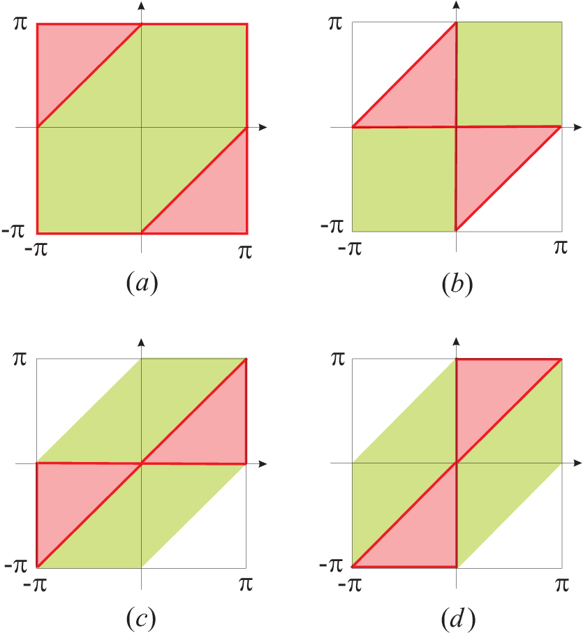
For ( in Theorem 3.4) there are 4 cases, depending on the parity of and .
a) If and are even, both and are good rays for any such that .
b) If and are odd, is a good ray for when belongs to the complement in of the two triangles (red area in Fig. 4b) with the vertices , and , respectively. Both and are good rays for when belongs to the union of the two squares and (green area in Fig. 4b).
c) If is even and is odd, is a good ray for when belongs to the complement in of the two triangles (red area in Fig. 4c) with the vertices and , respectively. Both and are good rays for when belongs to the union of the two open parallelograms (green area in Fig. 4c) with the generators , and , respectively.
d) If is odd and is even, is a good ray for when belongs to the complement in of the two triangles (red area in Fig. 4d) with the vertices and , respectively. Both and are good rays for when in the union of the two open parallelograms (green area in Fig. 4d) with the generators and , respectively.
In particular, if is on the positive imaginary axis, both and are good rays for when in case (a), in case (b), or in case (c), in case (d).
By definition, a good ray is not tangent to the vertical lines of and is not a Stokes line of either or . Since the angles between and vertical lines of have non-zero limits at the origin and at infinity, there is a lower bound for these angles on . This lower bound depends continuously on , hence there is a common lower bound for these angles for all rays in a proper subsector of a good sector (such that ).
The good sectors in Theorem 3.2 depend continuously on the arguments of the coefficients and of monomials and , except when a good sector degenerates to a ray that is a Stokes line of and an anti-Stokes line of .
The lower bounds for the angles between a good ray and vertical lines, and for the values of , depend continuously on the arguments of and , except when a good sector containing degenerates.
Now we show that a good ray for a monomial is admissible for the potential (2.2), with
for every positive .
Lemma 3.6.
Consider the polynomials , where , and . Let be a sector whose closure does not contain turning points of .
For every there exists depending on , such that for every :
(i) The set does not contain turning points of , and
(ii) If and are the vertical directions of and , respectively, then for
Proof.
We have for , so , and (i), (ii) hold when is large enough. ∎
4. PT-symmetric potentials and linear differential equations having solutions with prescribed number of non-real zeros
Hellerstein and Rossi asked the following question [9, Problem 2.71]. Let
| (4.1) |
be a linear differential equation with polynomial coefficient . Characterize all polynomials such that the differential equation admits a solution with infinitely many zeros, all of them real.
This problem was investigated in [42, 29, 28, 33, 38, 22]. Recently K. Shin [39] announced a description of polynomials of degree or such that equation (4.1) has a solution with infinitely many zeros, all but finitely many of them real. It turns out that equations (4.1) with this property are equivalent to (1.4) or (1.7) of the Introduction by an affine change of the independent variable.
Here we use the methods of [21, 19] to parametrize polynomials of degrees and such that equation (4.1) has a solution with prescribed number of non-real zeros.
We begin with degree .
Theorem 4.1.
For each integer there exists a simple curve in the plane which is the image of a proper analytic embedding of the real line and which has the following properties.
For every the equation
| (4.2) |
has a solution with non-real zeros. Real zeros belong to a ray and there are infinitely many of them. This solution satisfies .
The union coincides with the real part of the spectral locus of (1.4).
The projection ,
is a -to- covering map. The curves are disjoint, and for and , if and then .

Equation (4.2) is equivalent to the PT-symmetric equation (1.4) in the Introduction by the change of the independent variable . Computer experiments strongly suggest that the projection is -to- on the whole curve except one critical point of this projection, and that the whole curve lies above .
Fig. 5, taken from Trinh’s thesis [43] (see also [14]), shows a computer generated picture of the curves .
As a corollary from Theorem 4.1 we obtain that every eigenvalue of (1.4), when analytically continued to the left along the -axis, encounters a singularity for some . According to Theorem 2 of [19] this singularity is an algebraic ramification point.
Proof.
Consider the Stokes sectors of equation (4.2). We enumerate them counter-clockwise as where is bisected by the positive real axis. Consider the set of all real meromorphic functions whose Schwarzian derivatives are real polynomials of the form , and whose asymptotic values in the sectors are , respectively, where . Such functions are described by certain cell decompositions of the plane [19]. By a cell decomposition we understand a representation of a space as a union of disjoint cells. This union is locally finite, and the boundary of each cell consists of cells of smaller dimension. The -cells are points, vertices of the decomposition. The -cells are embedded open intervals, the edges, and the -cells are embedded open discs, faces of a decomposition. Two cell decompositions of a space are called equivalent if they correspond to each other via an orientation-preserving homeomorphism of .
To describe functions of the set , we begin with the cell decomposition of the Riemann sphere shown in Fig. 6.

It consists of one vertex at and three edges which are simple disjoint loops around and , so that the loop around is symmetric with respect to complex conjugation while the loops about and are interchanged by the complex conjugation. The point is outside the Fig. 6. The dotted line is not discussed here; it is needed for the future. Also for the future use, we assume that the loop around passes through the point , and that this loop is symmetric with respect to the reflection .
So our cell decomposition has one vertex, three edges and four faces. The faces are labeled by points and which are inside the faces. (So three faces are bounded by single edge each, while one face (labeled with ) is bounded by three edges).
Suppose now that we have a local homeomorphism such that the restriction
| (4.3) |
where , is a covering map, and . Then we preimage will be a cell decomposition of the plane . Now suppose that a cell decomposition of the plane is given in advance, and suppose that its local structure is the same as that of . This means that the faces of are labeled by elements of the set , and that a neighborhood of each vertex of can be mapped onto a neighborhood of the vertex of by an orientation-preserving homeomorphism, respecting the labels of the faces. Then there exists a local homeomorphism such that (4.3) is a covering map. We use the following cell decomposition to construct :

The five “ends” extend to infinity periodically. This cell decomposition depends on one integer parameter which is the number of -labeled faces between the neighboring “ramification points”. Only some face labels are shown but the reader can easily recover all other labels from the condition that in a neighborhood of each vertex is similar to a neighborhood of the vertex of . The dotted lines are not a part of our cell decomposition; they are preimages of the dotted line in Fig. 19, and are added for a future need. is symmetric with respect to the real line, this permits to make our local homeomorphism symmetric, that is . This construction defines the map up to pre-composition with a symmetric homeomorphism of the domain of . A fundamental result of R. Nevanlinna ensures that this homeomorphism can be chosen in such a way that is a meromorphic function which is real in the sense that . We refer to [19] for the discussion of this construction in our current context; in fact [19] contains a simple alternative proof of Nevanlinna’s theorem. Nevanlinna’s original proof is explained in modern language in [18]; the original paper of Nevanlinna is [36].
The meromorphic function is defined by the cell decomposition and parameter up to pre-composition with a real affine map . Furthermore, the Nevanlinna theory says that the Schwarzian derivative of is a polynomial of degree exactly (the number of unbounded faces of minus ). We pre-compose with a real affine map to normalize this polynomial to have leading coefficient and zero coefficient at . Thus
| (4.4) |
As is real, and are also real. Now is uniquely defined by the properties that it satisfies a differential equation (4.4), has asymptotic values in the sectors , respectively, and that equivalent to (Fig. 7 for ) by an orientation-preserving homeomorphism of the plane commuting with the reflection . The statement on asymptotic values implies that
Furthermore, depends analytically on , when is in the upper half-plane, and thus we obtain a real analytic map . This map is evidently invariant with respect to transformations , this is because the Schwarzian derivative in the right hand side of (4.4) does not change when is replaced by .
Thus for every , we have a one-parametric family of meromorphic functions, parametrized by , . Taking the Schwarzian derivative we obtain a map , . This map is known to be a proper real analytic immersion [2]. It is easy to see that it is injective: two solutions of the same Schwarz equation may differ only by post-composition with a fractional-linear map, and this fractional-linear map must be identity by our normalization of asymptotic values.
For the same reasons the images of are disjoint: for different , our functions have (topologically) different line complexes. The images of are our curves .
Now we prove that the union of coincides with the real part of the spectral locus of (1.7).
Our functions can be written in the form where and are two linearly independent solutions of equation (4.2) with some real and . We can choose and to be real entire functions. Condition that as implies that for so is an eigenfunction of the spectral problem
| (4.5) |
which is equivalent to (1.4) by the change of the independent variable .
Now, let be a real eigenvalue of the problem (4.5), a corresponding eigenfunction. Choose a point on the real line such that and normalize so that . Then is an eigenfunction with the same eigenvalue, so for some constant . Substituting gives that . So is real.
Let be a solution of the same equation as but satisfying . We normalize so that is real in the same way as we normalized . Then is a real meromorphic function whose Schwarzian derivative is a cubic polynomial with top coefficient , and the asymptotic values in are . We can change the normalization of multiplying it by any real non-zero constant. In this way we achieve that for some So belongs to the class .
Lemma 4.2.
.
Proof.
Let . Consider the cell decomposition . We have to prove that for some . To do this, we follow [19]. We first remove all loops from , and then replace each multiple edge by a single edge, and denote the resulting cell decomposition by . Notice that the cyclic order in Fig. 6 is consistent with the cyclic order of the Stokes sectors in the -plane. By [19, Proposition 6], this implies that the -skeleton of is a tree. This infinite tree is properly embedded in the plane, has faces, is symmetric with respect to the real line, and has two faces labeled with which are interchanged by the symmetry. Moreover, the faces of are in one-to-one correspondence with the Stokes sectors, and the face corresponding to is bisected by the positive ray. One can easily classify all trees with these properties. They depend of one integer parameter which is the distance between the ramification point in the upper half-plane and the ramification point on the real axis. Now we refer to [19, Proposition 7] that the tree uniquely defines the cell decomposition . This shows that for some .
Meromorphic function is defined by the cell decomposition and the parameter up to an affine change of the independent variable. Normalizing it as in (4.4) gives . ∎
We conclude that the union of our curves in the right half-plane coincides with the real part of the spectral locus of (4.5).
Now we study the shape of the curves . The boundary value problem (4.5) was considered by Shin [37], Delabaere and Trinh [43, 14]. The spectrum of this problem is discrete, simple and infinite. It is known [37] that for all eigenvalues of this problem are real and positive. It follows from this result that there are real analytic curves such that for each , is an eigenvalue of the problem (4.5), and . So the part of the real spectral locus in is the union of the graphs of .
Next we prove that the intersection of with the half-plane consists of and . For this purpose we study what happens to eigenvalues and eigenfunctions of the problem (4.5) as .
A different approach to the asymptotics as is used in [27]. We could use their Corollary 2.16 here instead of referring to Sections 2,3.
We substitute in (4.5) and put , where
The result is
| (4.6) |
where Choosing the positive and negative imaginary rays as our normalization rays and , we see that the normalization rays are admissible in the sense of Theorem 2.3. The Stokes complex of the binomial potential corresponding to (4.6) is shown in Fig. 3(a). According to Theorem 2.3, the spectrum of the problem (4.6) converges to the spectrum of the limit problem
| (4.7) |
This limit problem is equivalent to the self-adjoint problem
by the change of the variable . Convergence of the spectrum implies convergence of eigenfunctions uniform on compact subsets of the plane by Theorem 2.4. As varies from to , we can choose an eigenvalue which varies continuously, and the corresponding eigenfunction that varies continuously, and tends to an eigenfunction of (4.6). In the process of continuous change the number of non-real zeros of the eigenfunction cannot change because eigenfunctions cannot have multiple zeros. The conclusion of the theorem will now follow from the known properties of zeros of eigenfunctions of Hermitian boundary value problems, once we establish the following
Lemma 4.3.
As in (4.6) the non-real zeros of an eigenfunction cannot escape to infinity.
Notice that the real zeros of the eigenfunction do escape to infinity, as the limit eigenfunction has at most one real zero.
Proof.
Let be the eigenfunction constructed in Theorem 2.4 which depends continuously on . Let be the Sibuya solution corresponding to the positive ray. Then is a real meromorphic solution of the Schwarz equation and has asymptotic values in the sectors . As , and the Schwarzian of is of degree , we conclude that converges to the real axis, and the Riemann surface of must converge in the sense of Caratheodory [10, 45], to a Riemann surface with logarithmic branch points which can lie only over , where . To construct the cell decomposition corresponding to this limit Riemann surface, we consider two cases.
Case 1. To describe the limit function, we must replace in the original cell decomposition Fig. 6 two loops corresponding to , with a single loop around both of these points. This loop is shown by the dotted line in Fig. 6 and its preimage is shown by the dotted lines in Fig. 7. The original loops that separate - and - labeled faces from the face labeled must be removed. Performing this operation on the cell decomposition we see that the -skeleton breaks into infinitely many pieces. But there is only one piece that has four unbounded faces and thus can correspond to a meromorphic function whose Schwarzian derivative is a polynomial of degree . This limit decomposition is shown in Fig. 8.

This time both solid and dotted lines represent the edges of this decomposition. We see that the number of non-real zeros in the limit is the same as it was before the limit.

Now we want to find the preimage of the cell decomposition in Fig. 9 under the same function . There are several ways to find this preimage. Let us choose for convenience , and express the loops in Fig. 9, in terms of the loops in Fig. 6, as elements of the fundamental group of . We denote the loops around , in Fig. 6 by , and let , be the upper and lower halves of the loop around , so that ( followed by ). Let and be the loops in Fig. 9. Then we have ( followed by ), , . See Fig. 10.

These relations permit us to draw the preimages of the loops in the -plane. The resulting picture is shown in Fig. 11.

When , we have a degeneration as before. The corresponding cell decomposition is obtained by replacing preimages of the loops and by the preimages of the dotted line. The resulting cell decomposition is shown in Fig. 12.

We see that the limit function still has non-real zeros, and one real zero. This completes the proof of the lemma, and of Theorem 4.1. ∎
This proof shows that corresponds to the lower branch of while corresponds to the upper branch.
∎
Theorem 4.4.
Proof.
By the results of Gundersen [28, 29], all solutions have infinitely many zeros, and the coefficients of are real. By a real affine change of the variable we achieve that . As almost all zeros are real, our solution must tend to zero in both directions of the imaginary axis. So is an eigenvalue of the problem (4.5). Let be a real eigenfunction and a real solution of our equation that is linearly independent of . Then the ratio is a meromorphic function which is a local homeomorphism, and has asymptotic values in , respectively. After a real affine change of the independent variable, this function will belong to the class defined in the proof of Theorem 4.1. ∎
Now we state analogous results for quartic oscillators. There are two different real two-parametric families in which solutions with finitely many non-real zeros can occur [39].
| (4.8) |
| (4.9) |
studied in [4]. Here is an integer. Problem 4.9 is quasi-exactly solvable, which means that there are eigenfunctions of the form , where is a polynomial of degree .
The families (4.8) and (4.9) are equivalent to the PT symmetric families (1.7) and (1.8-1.9) of the Introduction via the change of the independent variable .
Theorem 4.5.
The real part of the spectral locus of (4.8) consists of disjoint smooth connected analytic surfaces , properly embedded in . For , the eigenfunction has non-real zeros. Each of these surfaces is homeomorphic to a punctured disc. Projection has the following properties: It is a -to- covering over some neighborhood of the -axis, and for , the preimage of every line is compact and homeomorphic to a circle.
Proof.
We follow the same pattern as in the proof of Theorem 4.1. There are Stokes sectors, , which we enumerate anticlockwise, beginning from the sector in the first quadrant.
If where is a real eigenfunction and is a real linearly independent solution of the same equation, then has asymptotic values in the sectors . Here , and must belong to .
If , we can choose with the additional symmetry with respect to the imaginary axis, which gives , so and belong to the same half-plane of . The same situation persists for all real because depend continuously on and never cross the real line. The real affine group acts on by post-composition; this corresponds to the change of normalization of and . So we can always choose the normalization so that .
Notice that after this normalization condition corresponds to See Remark 4.6 after the proof.
Consider the cell decomposition of the Riemann sphere (the range of ) shown in Fig. 13. It consists of one vertex at and four disjoint loops around and that are interchanged by the symmetry.

Now consider the cell decomposition of the plane (with labeled faces) shown in Fig. 14. It is locally similar to , and depends on one integer parameter which is the number of -labeled faces between the adjacent “ramification points”.

As in Theorem 4.1, Nevanlinna theory gives for each a family of meromorphic functions which have non-real zeros and satisfy the Schwarz equation of the form
| (4.10) |
with real .
Classification result for symmetric trees with faces in [19] ensures that all equations (4.1) having a solution with infinitely many real zeros and non-real zeros are equivalent to equations which arise from our families .
This also has an implication that there is “no monodromy” in our families : when traverses a loop around , we return with the same function we started with. Indeed, in the process of continuous deformation the number of non-real zeros cannot change, and there is only one suitable cell decomposition for every .
Thus our family is homeomorphic to a punctured disc. Taking the coefficients of the Schwarzian defines an analytic embedding of to . This is our surface . The surfaces are disjoint and properly embedded for the same reasons as in the proof of Theorem 4.1.
To study the shape of these surfaces in , we first notice that for , the eigenvalue problem obtained from (4.8) by rotation is Hermitian. It follows that the intersection with the plane consists of the disjoint graphs of two analytic functions defined for all real , and that . Another simple property of the surface is that it is symmetric with respect to change , which follows by changing in the equation.
Now we study the asymptotic behavior of for . In the equation (4.8) we set , where satisfies
| (4.11) |
and obtain
| (4.12) |
where
and
Expressing and from equations (4.11) as functions of and substituting the result to the expression of we obtain
| (4.13) | |||||
| (4.14) |
Consider the curves from Theorem 4.1. It follows from their properties stated in Theorem 4.1, that for every , there exists , and .
Suppose that , and consider the curve in -plane parametrized by (4.13). Equation (4.12) satisfies the conditions of Theorem 4.1 of Section 2 (the Stokes complex corresponding to this equation is shown in Fig. 1(a), rotated by ), and the sectors containing the normalizing rays are stable. We conclude that the spectrum of (4.12) tends to the spectrum of the cubic
| (4.15) |
The spectrum of the cubic with parameter has at least one eigenvalue which is real and such that the corresponding eigenfunction has non-real zeros. As is an isolated point of this spectrum, and the spectrum of (4.12) is symmetric with respect to the real axis, we conclude that there is an eigenvalue of (4.12) which is real, and the corresponding eigenfunction has non-real zeros.
To ensure that the number of non-real zeros does not change in the limit, we make an argument similar to that in the proof of Theorem 4.1, the degeneration of the cell decomposition is shown in Fig. 15.

We conclude that projection of our surface contains a piece of the curve (4.13) for .
Now suppose that . We claim that there are no points on with and on the curve (4.13). Proving this by contradiction, we suppose that there is a sequence such that belong to the curve (4.13). Then Theorem 2.3 implies that the sequence related to the by (4.14), has the property that tends to a real eigenvalue of the cubic oscillator (4.15). Then the corresponding eigenfunction tends to an eigenfunction of the cubic with non-real zeros. This is a contradiction because , so our claim is proved.
So the projection of on the plane looks as a paraboloid when . ∎
Fig. 16, which is taken from Trinh’s thesis shows a section of the surfaces by the plane . Similar pictures can be seen in [3, 13].

Computational evidence suggests that each has the shape of an infinite funnel with a sharp end stretching towards . This end probably corresponds to , where is the asymptotic value as in Figs. 13-14. as on as the picture in [13] suggests. For every real the section of by the plane is an oval that projects on the -axis -to-. We only proved that this section is compact for large enough. For the funnels are symmetric with respect to , lies above and is wider than .
Remark 4.6.
In general, it is hard to say anything explicit on the correspondence between the parameters in the potential and Nevanlinna parameter . Some information on this correspondence can be extracted from symmetry and degeneration considerations. In the beginning of the proof of Theorem we noticed that the line corresponds to the circle . We can determine now the sign of for inside and outside this circle. Degeneration used in the proof corresponds to convergence of to a real non-zero point. Formula (4.13) shows that when . So negative correspond to the exterior of the circle and positive to its interior.
Now we state the result about the second PT-symmetric family of quartics.
Theorem 4.7.
The real QES part of the spectral locus of (4.9) consists of simple disjoint analytic curves , , properly embedded curves which for project onto the ray -to-. When , the eigenfunction has non-real zeros.
The proof is completely similar to the proof of Theorem 4.1.
The problem of study of the whole real part of spectral locus of (4.9), as a two-parametric family with real seems quite interesting and challenging. A picture of the spectral locus for can be seen in [4].
Theorem 4.8.
The proof is similar to that of Theorem 4.4.
References
- [1] P. Alexandersson and A. Gabrielov, On eigenvalues of the Schrödinger operator with a polynomial potential with complex coefficients, in preparation.
- [2] I. Bakken, A multi-parameter eigenvalue problem in the complex plane. Amer. J. Math. 99 (1977), no. 5, 1015–1044.
- [3] C. Bender, M. Berry, P. Meisinger, Van M. Savage, M. Simsek, Complex WKB analysis of energy-level degeneracies of non-Hermitian Hamiltonians. J. Phys. A 34 (2001), no. 6, L31–L36.
- [4] C. Bender, S. Boettcher, Quasi-exactly solvable quartic potential. J. Phys. A 31 (1998), no. 14, L273–L277.
- [5] C. Bender and S. Boettcher, Real spectra in non-Hermitian Hamiltonians having symmetry, Phys. Rev. Lett., 80 (1998) 5243–5246.
- [6] C. Bender, S. Bottcher, V. M. Savage, Conjecture on the interlacing of zeros in complex Sturm-Liouville problems, J. Math. Phys. 41 (2000), no. 9, 6381–6387.
- [7] C. Bender, A. Turbiner, Analytic continuation of eigenvalue problems. Phys. Lett. A 173 (1993), no. 6, 442–446.
- [8] C. Bender and Tai Tsun Wu, Anharmonic oscillator. Phys. Rev. (2) 184 1969 1231–1260.
- [9] D. Brannan and W. Hayman, Research problems in complex analysis, Bull. London Math. Soc., 21 (1989) 1–35.
- [10] C. Carathéodory, Untersuchungen über die konformen Abbildungen von festen und veränderlichen Gebieten, Math. Ann., 72 (1912) 107–144.
- [11] E. Caliceti, S. Graffi and M. Maioli, Perturbation theory of odd anharmonic oscillators, Comm. Math. Phys., 75 (1980) 51–66.
- [12] E. Delabaere, F. Pham, Eigenvalues of complex Hamiltonians with -symmetry. I. Phys. Lett. A 250 (1998), no. 1-3, 25–28.
- [13] E. Delabaere, F. Pham, Eigenvalues of complex Hamiltonians with -symmetry. II. Phys. Lett. A 250 (1998), no. 1-3, 29–32.
- [14] E. Delabaere, Duc Tai Trinh Spectral analysis of the complex cubic oscillator. J. Phys. A 33 (2000), no. 48, 8771–8796.
- [15] P. Dorey, C. Dunning and R. Tateo, Spectral equivalences, Bethe ansatz equations, and reality properties in PT-symmetric quantum mechanics, J. Phys. A, 34 (2001) 5679–5704.
- [16] P. Dorey, C. Dunning and R. Tateo, A reality proof in PT-symmetric quantum mechanics, Czech. J. Phys., 54 (2004) 5.
- [17] P. Dorey, C. Dunning and R. Tateo, The ODE/IM correspondence arXiv:/hep-th/0703066v2.
- [18] A. Eremenko, Geometric theory of meromorphic functions, in the book: “In the tradition of Ahlfors and Bers III”, Contemp. math. 355, AMS, Providence, RI, 2004. Expanded version: www.math.purdue.edu/eremenko/dvi/mich.pdf
- [19] A. Eremenko, A. Gabrielov, Analytic continuation of eigenvalues of a quartic oscillator, Comm. Math. Phys., v. 287, No. 2 (2009) 431-457.
- [20] A. Eremenko and A. Gabrielov, Irreducibility of some spectral determinants, arXiv:0904.1714.
- [21] A. Eremenko A. Gabrielov and B. Shapiro, Zeros of eigenfunctions of some anharmonic oscillators, Ann. Inst. Fourier, Grenoble, 58, 2 (2008) 603-624.
- [22] A. Eremenko and S. Merenkov, Nevanlinna functions with real zeros, Illinois J. Math., 49, 3-4 (2005) 1093–1110.
- [23] M. A. Evgrafov and M. V. Fedorjuk, Asymptotic behavior of solutions of the equation as in the complex -plane. (Russian) Uspehi Mat. Nauk 21 1966 no. 1 (127), 3–50.
- [24] M. V. Fedoryuk, Asymptotic analysis. Linear ordinary differential equations. Springer-Verlag, Berlin, 1993.
- [25] G. M. Goluzin, Geometric theory of functions of a complex variable, AMS, Providence, RI, 1969.
- [26] S. Graffi, V. Grecchi and B. Simon, Borel summability: application to the anharmonic oscillator, Phys. Let., 32B, 7 (1970) 631–634.
- [27] V. Grecchi, M. Maioli and A. Martinez, Padé summability of the cubic oscillator, J. Math. Phys. A: Math. Theor. 42 (2009) 425208.
- [28] G. Gundersen, On the real zeros of solutions of where is entire, Ann. Acad. Sci. Fenn. Math. 11, 1986 276–294.
- [29] G. Gundersen, Solutions of that have almost all real zeros, Ann. Acad. Sci. Fenn. Math., 26 (2001) 483–488.
- [30] H. Habsch, Die Theorie der Grundkurven und das Äquivalenzproblem bei der Darstellung Riemannscher Flächen, Mitteilungen Math. Sem. Giessen, 42 (1952).
- [31] C. Handy, Generating converging bounds to the (complex) discrete states of the Hamiltonian, J. Phys. A: Math. Gen. 34 (2001) 5065–5081.
- [32] J. Heading, An introduction to phase-integral methods, Methuen, London; John Wiley, NY 1962.
- [33] S. Hellerstein and J. Rossi, Zeros of meromorphic solutions of second order linear differential equations, Math. Z., 192 (1986) 603–612.
- [34] E. Hille, Lectures on ordinary differential equations. Addison-Wesley Publ. Co., Reading, Mass.-London-Don Mills, Ont. 1969
- [35] D. Masoero, Poles of intégrale tritronqueée and anharmonic oscillators. A WKB approach, J. Phys. A: Math. Theor. 43 095201 .
- [36] R. Nevanlinna, Über Riemannsche Flächen mit endich vielen Windungspunkten, Acta Math., 58 (1932) 295–373.
- [37] K. Shin, On the reality of the eigenvalues for a class of PT-symmetric oscillators, Comm. Math. Phys., 229 (2002) 543–564.
- [38] K. Shin, New polynomials for which has a solution with almost all real zeros. Ann. Acad. Sci. Fenn. Math. 27 (2002), no. 2, 491–498.
- [39] K. Shin, All cubic and quartic polynomials for which has a solution with infinitely many real zeros and at most finitely many non-real zeros, Abstracts AMS 1057-34-26 (Lexington, KY, March 27-28, 2010).
- [40] Y. Sibuya, Global theory of a second order linear ordinary differential equation with a polynomial coefficient, North-Holland, Amsterdam–Oxford; American Elsevier, NY, 1975.
- [41] B. Simon and A. Dicke, Coupling constant analyticity for the anharmonic oscillator, Ann. Physics 58 (1970), 76–136.
- [42] E. Titchmarsh, Eigenfunction expansions associated with second order differential equations, vol. 1, second edition, Oxford, Oxford UP, 1962.
- [43] Duc Tai Trinh, Asymptotique et analyse spectrale de l’oscillateur cubique, These, 2002.
- [44] Duc Tai Trinh, On the Sturm–Liouville problem for the complex cubic oscillator, Asymptot. Anal. 40 (2004) 211-234.
- [45] L. Volkovyski, Converging sequences of Riemann surfaces, Mat. Sbornik, 23(65) (1948), N 3, 361–382. (Russian). Oxford UP, 1989.