Event shapes in $e^{+}e^{-}$ collisions provide some of the best ways to test QCD and the standard model. At high energies, where QCD is perturbative, event shapes lead to some of the world’s most precise measurements of the strong coupling constant $\alpha_{s}$. Recently, a number of theoretical advances have led to renewed interest in event shapes and the $\alpha_{s}$ measurements. First, the NNLO fixed order Feynman diagrams were calculated [1, 2, 3, 4]. This allowed the prediction of all event shapes to order $\alpha_{s}^{3}$. Second, advances [5, 6, 7] in Soft-Collinear Effective Theory (SCET) [8, 9, 10] have allowed resummation of the large logarithmic corrections to thrust to N³LL accuracy [11]. Previous calculations were at NLO [12] and NLL [13]. Very recently, a full effective field theory analysis of a single event shape, thrust, has been completed [14], including additionally non-perturbative considerations. The resulting $\alpha_{s}$ extraction is competitive with the PDG world average [15], however it differs significantly from measurements using lattice QCD and $\tau$ decays (see [16] for a review).

Although the $\alpha_{s}$ measurement with thrust is extremely precise, there are many reasons to study additional event shapes as well. The main advantage is that there may be systematic effects in a single event shape pulling $\alpha_{s}$ in a certain direction, which are not universal. In fact, as observed in [17] from an NLL+NNLO analysis, there seem to be two classes of event shapes, the first including thrust, the $C$-parameter and total jet broadening, while the second includes heavy jet mass, wide jet broadening and the two-to-three jet transition parameter $y_{3}$. The values of $\alpha_{s}$ extracted from the two classes at NLL+NNLO tend to have around a 5% systematic difference which the authors attribute to missing higher order corrections. In a recent world average of $\alpha_{s}$ [16], the thrust measurement using SCET was not included because of a concern over precisely this kind of systematic uncertainty. In this paper, we correct that concern with a N³LL calculation of an event shape from the second class, heavy jet mass.

In addition to being useful for measuring $\alpha_{s}$, the heavy jet mass distribution allows us to explore other aspects of resummation. Indeed, there are few hadronic observables which have been calculated this accurately and for which there is data. Heavy jet mass involves a soft function which cannot be written in terms of only a single scale. These types of soft functions promise to play an important role in resummation at hadron colliders and only beginning to be explored [19, 20, 21]. We will discuss constraints on the soft function, and perform a numerical study of the parts that are not known, similar to what was done in [11] and [22].

Hadronization is another issue which having a second event shape may help understand. In the fit to $\alpha_{s}$ with the thrust distribution [11], it was observed that a decrease in $\alpha_{s}$ could be compensated for with a single non-perturbative parameter with only a small effect on the $\chi^{2}$ of the fit. Having another observable for which the same non-perturbative parameters can be fit can possibly remove this flat direction. The hadronization issue is also important for Monte Carlo simulations. With a more accurate theoretical calculations, we can explore whether the approximations in pythia [23] allow for an adequate description of thrust and heavy jet mass simultaneously.

As a brief outline of our findings, we begin in Section 2 with an overview of the SCET distributions. The hemisphere soft function is studied and singular terms in the heavy jet mass distribution are compared to the fixed order calculation in Section 3. We found a mild inconsistency with the analytic results from SCET and the numerical calculations of the NLO and NNLO distributions. After completing the original study, we were able to resolve this inconsistency, which was due to Monte Carlo convergence problems, by taking a very low numerical infrared cutoff, as discussed in a note added at the end of this paper. In Section 4 we fit for $\alpha_{s}$. The fit for heavy jet mass to the lep data from aleph [24] leads to $\alpha_{s}(m_{Z})=0.1220\pm 0.0031$. This value is higher than the value from thrust using exactly the same technique, $\alpha_{s}(m_{Z})=0.1175\pm 0.0026$. Assuming 100% correlation gives an average value of $\alpha_{s}(m_{Z})=0.1193\pm 0.0027$ which is very close to the recent average in [16]. We also find that convergence of the perturbation series for heavy jet mass with resummation is, like for thrust, significantly better than the convergence of the fixed order calculation. In Section 5, a comparison of the data to pythia shows that while pythia agrees with the thrust data almost perfectly, it has trouble matching the heavy jet mass distribution. Moreover, the hadronization corrections in pythia move the curve in the wrong direction for heavy jet mass. Concluding that the Monte Carlo hadronization model is incompatible with the high precision theoretical calculation, we explore non-perturbative corrections in SCET with a simple shape function. We find that to the order we are working, this simple shape function cannot simultaneously describe the thrust and heavy jet mass distributions. We provide an expanded summary, discussion and comparison to previous results in Section 6.

Thrust and heavy jet mass are defined as follows. One first finds the thrust axis, through

where the sum is over all momentum 3-vectors $\mathbf{p}_{i}$ in the event, and the maximum is over all unit 3-vectors ${\mathbf{n}}$. We use $\tau=1-T$ to measure thrust. Once the thrust axis is known, it can be used to split the event into two hemispheres. We define $P_{L}^{\mu}$ and $P_{R}^{\mu}$ to be the four momenta of the sum of all the radiation going into each hemisphere, and $M_{L}=\sqrt{P_{L}^{2}}$ and $M_{R}=\sqrt{P_{R}^{2}}$ to be the hemisphere masses. Heavy jet mass $\rho$ is defined as the larger of the two hemisphere masses squared, normalized to the the center of mass energy $Q$,

When $\rho$ is small, $\tau$ is also small, both hemisphere masses are small, and the event appears to have two back-to-back pencil-like jets. In this threshold limit, the thrust axis aligns with the jet axis and $Q^{2}\tau$ approaches the sum of the two hemisphere masses squared $M_{L}^{2}+M_{R}^{2}=Q^{2}\tau+{\mathcal{O}}(\tau^{2})$.

It follows that both thrust, up to power corrections, and heavy jet mass can be written as integrals over the doubly differential hemisphere mass distribution:

In SCET, the doubly differential hemisphere mass distribution is calculable in the threshold limit. The appropriate factorization theorem in SCET was first derived in [5] for the related process of $t\bar{t}$ production. This theorem was then shown to allow for the calculation of event shapes in [6], where matched and resummed thrust and heavy jet mass distributions in SCET were first presented. Previously, resummation of heavy jet mass was only possible at NLL accuracy [13]. The first event shape resummed to N³LL was thrust, in [11]. Monte Carlo based hadronization corrections were included in [25] to produce a strong model-independent gluino mass bound. Recently, power corrections for thrust were studied within the effective field theory approach in [14].

The factorization theorem allows us to write the hemisphere mass distribution as

The subscript on $\sigma_{2}$ is a reminder that this expression holds in the two-jet region. Here, $H(Q^{2},\mu)$ is the hard function. It is calculated in matching SCET to QCD and contains information about the modes of QCD that are not in SCET. $J(p^{2},\mu)$ is a jet function. It is derived in a matching calculation from a theory with soft and collinear modes to a theory with just soft modes. The hard function was calculated in [26] and the jet functions in [7]. Finally, $S(k_{L},k_{R},\mu)$ is the hemisphere soft function which is derived from integrating out the remaining soft modes.

The doubly differential hemisphere mass distribution, Eq. (5), is observable, and therefore must be independent of renormalization group scale $\mu$. Demanding $\mu$-independence leads to a renormalization group equation which is easiest to express in Laplace space, where the convolutions turn into products. The Laplace transform is defined by

which can be applied to the differential cross section and to the jet and soft functions separately. We generally express the Laplace transformed distributions as functions of ${\color[rgb]{0.6,0,0}L_{1}}=\ln(\mu{\color[rgb]{0.6,0,0}\nu_{L}}e^{\gamma_{E}})$ and ${\color[rgb]{0.6,0,0}L_{2}}=\ln(\mu{\color[rgb]{0.6,0,0}\nu_{R}}e^{\gamma_{E}})$. Since the entire $\mu$-dependence of the hard and jet functions is known, the $\mu$-dependence of the soft function is completely fixed by renormalization group invariance (see [11] for more details). The result is that the hemisphere soft function itself factorizes into the form [5, 6, 27, 22]

where all the $\mu$-dependence is contained in the function $\widetilde{s}_{\mu}({{\color[rgb]{0.6,0,0}L}},\mu)$ which is known to N³LL accuracy. Since ${{\color[rgb]{0.6,0,0}L_{1}}}-{{\color[rgb]{0.6,0,0}L_{2}}}=\ln({\color[rgb]{0.6,0,0}\nu_{L}}/{\color[rgb]{0.6,0,0}\nu_{R}})$, the function $\widetilde{s}_{f}({{\color[rgb]{0.6,0,0}L_{1}}}-{{\color[rgb]{0.6,0,0}L_{2}}})$ is $\mu$-independent. We discuss the soft function more in the next section.

Putting together the hard and jet functions with the soft function written in this way produces an analytic expression for the doubly differential jet mass distribution. For thrust, the result is [11]

with $\eta=4A_{\Gamma}(\mu_{j},\mu_{s})$ and the thrust soft function $\widetilde{s}_{T}({{\color[rgb]{0.6,0,0}L}},\mu)$ is defined by

The definitions of the RG kernels $A_{\Gamma}(\nu,\mu)$ and $S(\nu,\mu)$ as well as the fixed order hard and jet functions, $H(Q^{2},\mu)$ and $\widetilde{j}({{\color[rgb]{0.6,0,0}L}},\mu)$ and their anomalous dimensions can be found in [11]. Note that only one value of the unknown function $\widetilde{s}_{f}({{\color[rgb]{0.6,0,0}L}})$ is required for thrust.

For heavy jet mass, the distribution is similar

where $\eta_{1}=\eta_{2}=2A_{\Gamma}(\mu_{j},\mu_{s})$. In contrast to thrust, for heavy jet mass the full functional form of $\widetilde{s}_{f}({{\color[rgb]{0.6,0,0}L}})$ is needed. For N³LL precision, we need to know the hemisphere soft function, and hence $\widetilde{s}_{f}({{\color[rgb]{0.6,0,0}L}})$ to two-loop order (NLO). Actually, to this order, we only need one projection of the hemisphere soft function. For three-loop matching (NNLO), we need an additional projection. These projections will be discussed in the next section.

One interesting feature of the hemisphere mass distribution is that the soft interference effects in $\widetilde{s}_{f}({{\color[rgb]{0.6,0,0}L}})$ are only relevant at $\alpha_{s}^{2}$, which is appropriate for N³LL resummation. Up to NNLL accuracy, the doubly differential distribution is simply the product of the mass distributions in the two hemispheres. Explicitly,

where

and $\eta=2A_{\Gamma}(\mu_{j},\mu_{s})$. Since, for NNLL resummation, the hard and jet functions are only needed to ${\mathcal{O}}(\alpha_{s})$, the square-roots above simply mean take one half of the $\alpha_{s}$ pieces. The fact that the distribution splits up in this way was observed at NLL level in [6], and is essential to the traditional NLL resummation [13]. This simplified factorization suggests that it may be possible to calculate observables involving many more jets with NNLL resummation without having to disentangle soft interference effects. Note that this factorization does not guarantee that large logs of $M_{L}^{2}/M_{R}^{2}$ can be resummed. However, it is possible that the calculation of observables with only one scale, such as the sum of many jet masses, or a maximal jet mass, will simplify with SCET.

The hemisphere soft function has been studied briefly in [5, 6, 27] and more thoroughly in [22]. It is a function of two scales, $k_{L}$ and $k_{R}$ as well as the renormalization group scale $\mu$. If ${\color[rgb]{0.6,0,0}n_{L}^{\mu}}$ is the direction of the left hemisphere and $k^{\mu}_{L}$ is the sum of the momenta of all the soft radiation entering this hemisphere, then $k_{L}$ is the component of $k_{L}^{\mu}$ backwards to ${\color[rgb]{0.6,0,0}n_{L}^{\mu}}$. That is $k_{L}=(k_{L}\hskip-1.00006pt\cdot\hskip-1.00006pt{\color[rgb]{0.6,0,0}n_{L}})$. $k_{R}$ is defined analogously. The soft function can be factorized into a perturbative, partonic part, and non-perturbative contribution which has support of order $\Lambda_{\mathrm{QCD}}$. For now we deal only with the perturbative part, discussing non-perturbative effects in Section 5.

As we have noted, the soft function itself factorizes.

where $\widetilde{s}({\color[rgb]{0.6,0,0}L_{1}},{\color[rgb]{0.6,0,0}L_{2}},\mu)$ is the Laplace transform of $S(k_{L},k_{R},\mu)$, as in Eq. (6), and ${\color[rgb]{0.6,0,0}L_{1}}=\ln(\mu{\color[rgb]{0.6,0,0}\nu_{L}}e^{\gamma_{E}})$, ${\color[rgb]{0.6,0,0}L_{2}}=\ln(\mu{\color[rgb]{0.6,0,0}\nu_{R}}e^{\gamma_{E}})$. The function $\widetilde{s}_{\mu}({{\color[rgb]{0.6,0,0}L}},\mu)$ is completely fixed by RG invariance in terms of the hard and jet anomalous dimensions. It can be calculated in perturbation theory by demanding Eq. (10) be independent of $\mu$. This gives

The $\mu$-independent part $\widetilde{s}_{f}({{\color[rgb]{0.6,0,0}L}})$ must satisfy a number of constraints, as discussed in [22].

First of all, since the soft function is symmetric in the two hemispheres, $\widetilde{s}_{f}({{\color[rgb]{0.6,0,0}L}})$ must be an even function of ${{\color[rgb]{0.6,0,0}L}}$. Second of all, we know the function to order $\alpha_{s}$ by explicit calculation. Writing

the one-loop result is that

The authors of [22] also observed that $\widetilde{s}_{f}({{\color[rgb]{0.6,0,0}L}})$ is constrained by the non-Abelian exponentiation theorem. Non-Abelian exponentiation implies constraints on powers of logarithms of $\mu$ in the full soft function. These constraints are satisfied by the explicit solution, since $\widetilde{s}_{\mu}({{\color[rgb]{0.6,0,0}L}},\mu)$ is an exponential. The theorem also restricts the $C_{F}^{n}$ color structure in the soft function to be completely determined by the one-loop result, Eq. (16). Beyond this, however, $\widetilde{s}_{f}({{\color[rgb]{0.6,0,0}L}})$ is unconstrained. It may even have more general dependence on ${{\color[rgb]{0.6,0,0}L}}$ than logarithms. To determine $\widetilde{s}_{f}({{\color[rgb]{0.6,0,0}L}})$, we must calculate the soft function perturbatively. The one-loop calculation has been done but the two-loop calculation, which is required for N³LL resummation, has not.

A simple alternative to calculating $\widetilde{s}_{f}({{\color[rgb]{0.6,0,0}L}})$ at NNLO is to extract projections of $\widetilde{s}_{f}({{\color[rgb]{0.6,0,0}L}})$ from numerical comparisons to event shape calculations in full QCD. For example, thrust is only sensitive to $\widetilde{s}_{f}(0)$. Writing

and comparing to Eq. (16), we see that ${\color[rgb]{0,0,0.8}c^{S}_{1}}=-C_{F}\pi^{2}$. The two-loop constant was determined numerically in [11] with the use of the event 2 program [28]. The result is

This is in conflict with the prediction from non-Abelian exponentiation, which requires the $C_{F}^{2}$ factor be $\frac{1}{2}\pi^{4}C_{F}^{2}=48.7C_{F}^{2}$. The two-loop constant was also determined in [22], using the same technique but imposing non-Abelian exponentiation. They found

The two results agree, except for the $C_{F}^{2}$ term. Indeed, the $C_{F}^{2}$ term seems to indicate a disagreement between the numerical results of the event 2 program and the prediction from non-Abelian exponentiation. Since the uncertainty in Eq (18) is too small to explain this disagreement, it is reasonable also to expect the other color structures to be off. We should therefore allow for a systematic uncertainty on these fits in addition to what is presented, which is essentially a statistical uncertainty associated with the fit. We discuss this more below.

Event shapes other than thrust are sensitive to the form of $\widetilde{s}_{f}({{\color[rgb]{0.6,0,0}L}})$, not just $\widetilde{s}_{f}(0)$. This can be seen, for example, by the form of the heavy jet mass distribution in Eq. (10). For N³LL resummation, the fixed order expansion is required to $\alpha_{s}^{2}$. The contribution at this order involving $\widetilde{s}_{f}({{\color[rgb]{0.6,0,0}L}})$ requires at most $\widetilde{s}_{f}{}_{2}({{\color[rgb]{0.6,0,0}L}})$, with the jet and hard functions at their tree-level values. Thus, the required projection of the $\widetilde{s}_{f}({{\color[rgb]{0.6,0,0}L}})$ for heavy jet mass is

The integral representation of ${\color[rgb]{0,0,0.8}c^{S}_{2\rho}}$ is suggestive of a deeper relation between heavy jet mass and the hemisphere mass distribution, however we do not have a physical explanation of why this particular moment appears. If $\widetilde{s}_{f}({{\color[rgb]{0.6,0,0}L}})$ is a polynomial, this moment is very simple. For example, if we assume

then

At NLO, the singular part of the heavy jet mass distribution only depends on $\widetilde{s}_{f}({{\color[rgb]{0.6,0,0}L}})$ through ${\color[rgb]{0,0,0.8}c^{S}_{2\rho}}$. Thus, we can fit ${\color[rgb]{0,0,0.8}c^{S}_{2\rho}}$ numerically the same way ${\color[rgb]{0,0,0.8}c^{S}_{2}}$ is fit with thrust.

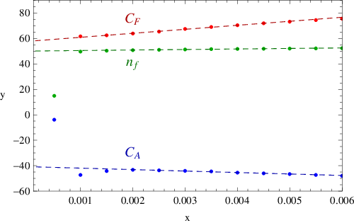
To determine ${\color[rgb]{0,0,0.8}c^{S}_{2\rho}}$ we use the same technique used in [11] for thrust, and in [22] for a one-parameter family of event shapes. The basic idea is that the singular part of the heavy jet mass distribution is known analytically, through SCET. The difference between the exact NLO heavy jet mass distribution and this singular part is finite and can be integrated numerically. This integral is then the total cross section at NLO minus the integral of the singular part which is calculable analytically and depends on the constants ${\color[rgb]{0,0,0.8}c^{S}_{2}}$ for thrust and ${\color[rgb]{0,0,0.8}c^{S}_{2\rho}}$ for heavy jet mass.

In more detail, the exact heavy jet mass distribution can be expanded as a series in $\alpha_{s}$

Each term in this series is singular at $\rho=0$. The singular parts can be written as a sum of distributions

The functions $D_{\delta}$, $D_{A}(\rho)$, $D_{B}(\rho)$, and $D_{C}(\rho)$ are calculable in SCET and we give them in Appendix C. Up to order $\alpha_{s}^{2}$, the only dependence on the unknown soft function coefficient ${\color[rgb]{0,0,0.8}c^{S}_{2\rho}}$ is in $D_{\delta}$, thus the shape of the singular part of the NLO distribution is known completely. The corresponding exact distributions in perturbative QCD have been calculated for $\rho>0$ analytically for the $A$ function, and numerically for the $B$ and $C$ functions. Since SCET produces the entire singular part of the distributions, the combination

should vanish at $\rho=0$. We show this difference separated by color structure in Figure 1. The $B$ functions are calculated using the Monte Carlo program event 2 [28] with $10^{10}$ events. Curiously, while the $C_{F}$ and $C_{A}$ color structures do not seem to go to $0$ as $\rho\to 0$, their sum does.

With these difference functions, it is straightforward to extract ${\color[rgb]{0,0,0.8}c^{S}_{2\rho}}$ as in [11] and [22]. Although the difference $\rho B(\rho)-\rho D_{B}(\rho)$ is regular at $\rho=0$, the two functions are separately divergent. Since $D_{B}(\rho)$ is only known numerically, the difference is numerically unstable at small $\rho$. To do the ${\color[rgb]{0,0,0.8}c^{S}_{2\rho}}$ extraction, we use the same procedure as in [11] and impose an lower bound and take the limit that the bound is removed. The extracted values as a function of this lower bound ${\rho_{\text{min}}}$ are shown in Figure 2. We then fit a line in the region $0.002\leq{\rho_{\text{min}}}\leq 0.005$ and extrapolate to ${\rho_{\text{min}}}=0$. The result is

Note that the $C_{F}$ and $C_{A}$ curves have problems at small ${\rho_{\text{min}}}$, in agreement with what is seen in Figure 1. Since the approach is linear up to around ${\rho_{\text{min}}}\sim 0.002$, it is likely that this divergence is an unphysical systematic problem with the Monte Carlo, and not due to low statistics or a discrepancy with theory. ¹¹ 1 We thank A. Hoang for a discussion of this point. As with ${\color[rgb]{0,0,0.8}c^{S}_{2}}$, non-Abelian exponentiation implies that the $C_{F}^{2}$ term should be $\frac{1}{2}\pi^{4}\approx 48.7$. Thus, our uncertainty of ${\color[rgb]{0,0,0.8}c^{S}_{2\rho}}$ from the extrapolation is probably too small and we will therefore inflate the errors by a factor of 5. (See also Eq. (50) and Figures 11 and 12 for an update.)

To calculate the heavy jet mass distribution to N³LL+NNLO accuracy, we must match to the NNLO fixed order distribution. This requires the singular parts of heavy jet mass to $\alpha_{s}^{3}$, that is, the function $D_{C}(\rho)$ in Eq. (24). To derive this, we do not need the finite part of the soft function at $\alpha_{s}^{3}$, $\widetilde{s}_{f}{}_{3}({{\color[rgb]{0.6,0,0}L}})$, since this piece only contributes to the $\alpha_{s}^{3}$ part of $D_{\delta}$, which is not required for matching. We do, however, need another projection of the $\alpha_{s}^{2}$ soft function, of the form

Again, we have no physical explanation of the intriguing integral definition in the second line. This projection also simplifies with a polynomial soft function. For example, with Eq (21)

The prediction from SCET for $D_{C}(\rho)$ with its explicit dependence only on ${\color[rgb]{0,0,0.8}c^{S}_{2\rho}}$ and ${\color[rgb]{0,0,0.8}c^{S}_{2\zeta}}$ is given in Appendix C. There are only three color structures which depend on ${\color[rgb]{0,0,0.8}c^{S}_{2\zeta}}$ at all.

In order to extract the ${{\color[rgb]{0.6,0,0}L}}$ dependence of $\widetilde{s}_{f}{}_{2}({{\color[rgb]{0.6,0,0}L}})$, we could attempt to fit ${\color[rgb]{0,0,0.8}c^{S}_{2\zeta}}$ with the shapes of the NNLO distributions. An alternative, as pursued by Hoang and Kluth in [22], is to use the other event shapes beyond thrust and heavy jet mass at NLO. These authors considered a weighted sum of the jet masses, $\tau_{\alpha}=\frac{2}{1+\alpha}(\alpha M_{L}^{2}+M_{R}^{2})/Q^{2}$. This form leads to a singular distribution which depends on $\widetilde{s}_{f}{}_{2}(\ln\alpha)$, hence combining event shapes with different $\alpha$ can probe the entire function $\widetilde{s}_{f}{}_{2}({{\color[rgb]{0.6,0,0}L}})$. Their fits show good agreement with the form

which they have argued is likely to be the exact 2-loop soft function. We will therefore assume this form of the soft function as well, in order to proceed with the N³LL+NNLO $\alpha_{s}$ fits. ²² 2 There is a subtlety about these $\tau_{\alpha}$ event shapes because of non-global logarithms [30]. For example, for very large or small $\alpha$, these event shapes reduce to the left or right hemisphere mass, which are known to have non-global logs. Since $\tau_{\alpha}\to 0$ forces the massless dijet threshold, in which the SCET factorization theorem is derived, only up to corrections of order $\ln\alpha$, it is not completely clear that SCET will reproduce all of the $\alpha$-dependence of the singular terms in $\tau_{\alpha}$.

With this soft function and the thrust fit values in Eq. (18), our fit for ${\color[rgb]{0,0,0.8}c^{S}_{2\rho}}$ translates into a fit for ${\color[rgb]{0,0,0.8}c^{S}_{2L}}$ (cf. Eq.(22) with ${\color[rgb]{0,0,0.8}c^{S}_{2Q}}=0$) The result is

Using a similar technique, but imposing the constraint from non-Abelian exponentiation, Hoang and Kluth found results consistent with ours

Note that for ${\color[rgb]{0,0,0.8}c^{S}_{2L}}$, the $C_{F}^{2}$ coefficient comes out to be consistent with the prediction from non-Abelian exponentiation. Since ${\color[rgb]{0,0,0.8}c^{S}_{2L}}$ comes from the difference between the values extracted from thrust and the values extracted from heavy jet mass, the systematic problem with event 2 may be cancelling in the difference. Thus, we will inflate our uncertainties on ${\color[rgb]{0,0,0.8}c^{S}_{2L}}$ by only a factor of $2$.

In summary, for the rest of this paper, we will take

so that

The uncertainty on $\alpha_{s}$ due to the uncertainty on these numbers will be included in the fits.

Before moving on the $\alpha_{s}$ extraction, we can compare the SCET prediction for the singular parts of the NNLO distribution to the exact results, as was done for thrust in [11]. To do this, we use $D_{C}(\rho)$ from Appendix C with the substitutions in Eq. (36). This lets us compare to the $C$ functions in the NNLO distribution, from [29]. Plots of $\rho D_{C}$ and $\rho C$ are shown in Figure 3 as functions of $\log\rho$. The uncertainty on ${\color[rgb]{0,0,0.8}c^{S}_{2}}$ and ${\color[rgb]{0,0,0.8}c^{S}_{2L}}$ is included, but not visible in these plots. Although the agreement is not perfect at very small $\rho$, it is expected to improve, as we seen for thrust in [11], as the the infrared cutoff used in the NNLO calculation is reduced from the value $y_{0}=10^{-5}$ used here. A version of this plot with cutoff $y_{0}=10^{-7}$ has been included as Figure 13, confirming our expectations.

The difference between the full NNLO distribution and its singular parts, as in Eq. (25), is shown in Figure 4. These curves, for all color structures, should go to zero at $\rho=0$. For most of the color structures, this looks plausible, although the $1/N^{2}$ color structure, corresponding to the $\alpha_{s}^{3}C_{F}^{3}$ coefficient in the heavy jet mass distribution which is fixed by non-Abelian exponentiation, looks a bit suspicious. Because this constant is known, we have not included an associated uncertainty. The discrepancy is likely due to the infrared cutoff $y_{0}=10^{-5}$ used for these plots (an update with $y_{0}=10^{-7}$ is included as Figure 14). Note that even if the Ansatz in Eq. (33) were wrong, a general dependence on ${\color[rgb]{0,0,0.8}c^{S}_{2\zeta}}$ will only affect some of the color structures, and even then would only generate an overall up or down shift in these curves (cf. the form of $D_{C}$ in Eq. (70)).

In the previous section, we determined the unknown coefficients in the hemisphere soft function and checked the singular terms against the exact NLO and NNLO heavy jet mass distributions. Now we are ready to compare to data and fit for the strong coupling constant $\alpha_{s}$. The procedure we follow is identical to the procedure used for thrust in [11], so we refer the reader to that paper for missing details.

For heavy jet mass, as for thrust, we match to the fixed order distribution via

with

and $D_{A},D_{B}$ and $D_{C}$ are given in Appendix C. The $A$ function is known analytically, and is the same as for thrust (see [6]). For $B(\rho)$ we use the output of event 2 [28], and for $C(\rho)$ we use the NNLO calculation which has been provided to us by the authors of [3]. We normalize to the total hadronic cross section at order $\alpha_{s}^{2}$, which is

Since the data is binned, what we actually use for the theory prediction is the difference between the integrated heavy jet mass distribution evaluated at the bin edges: $R_{\rho}(\rho_{2})-R_{\rho}(\rho_{1})$. Our fit ranges are chosen to be the same as in [18], so that we can use their values for the systematic experimental uncertainties.

The left panel of Figure 5 shows a comparison of the theory prediction for heavy jet mass to the aleph data at 91.2 GeV. These curves use the default scale choices

These scales are the natural ones to minimize the large logarithms, and can be read off the formula in Eq. (10). The best fit value of $\alpha_{s}$ for heavy jet mass is $\alpha_{s}(m_{Z})=0.1214$. We show also in the same figure, the heavy jet mass distribution for $\alpha_{s}(m_{Z})=0.1168$, which is the value of $\alpha_{s}$ derived in [11] from the fit to the thrust distribution at the same energy. In the right panel of Figure 5, we show a comparison to data for thrust, with the same values of $\alpha_{s}$. Overall, the fit to thrust is a much better fit. For heavy jet mass, the best fit gives $\chi^{2}$/d.o.f.=67/9 using statistical uncertainties only, while for thrust, $\chi^{2}$/d.o.f.=32.5/13. The relatively poor fit for heavy jet mass can be plainly seen in the figure. For thrust, the relative distribution is flat over the fit range (dashed curve, right panel), while for heavy jet mass, it is increasing (solid curve, left panel). This coordinates with the relatively larger power corrections that we will find in the next section.

Next, we look at the uncertainties on the theoretical prediction. As with thrust, in [11], we consider first separate variations of $\mu_{h}$, $\mu_{j}$, $\mu_{s}$ and the scale $\mu_{m}$ where the matching is done by factors of $2$. Figure 6 shows the effect of the envelope of these variations on the heavy jet mass distribution, for four orders in perturbation theory. We use the same definitions for the various orders as in [11]:

The first three orders correspond to traditional counting in renormalization-group improved perturbation theory, while 4^thorder simply uses all the available information.

Next, we consider, the separate variations. The bands in the first four panels of Figure 7 show the effect of the scale uncertainties. The bottom two panels of Figure 7 show the effect of the more natural correlated and anti-correlated scale variations introduced in [11]. The correlated variation is defined to hold $\mu_{j}/\mu_{s}$ fixed. So we vary

This probes the upper and lower limits on $\mu_{j}$ and $\mu_{s}$, but avoids the unphysical region where $\mu_{s}<\mu_{j}$ or $\mu_{h}<\mu_{j}$. The orthogonal anti-correlated variation is defined to hold $\mu_{j}^{2}/(Q\mu_{s})$ fixed. It is

This is independent from the correlated mode but again avoids unphysical scale choices.

Overall, we find good convergence order-by-order in perturbation theory. However, some of the higher-order scale variations are outside of the range of the lower orders. This was not the case for thrust, where the central value of the prediction was much more stable. Nevertheless, for both thrust and heavy jet mass, the complete perturbative uncertainty, defined as the envelope of the various variations (that is, the maximum and minimum over them) does have the higher-order bands contained within the lower order bands, as can be seen in Figure 6.

Next, we fit the theoretical prediction to the aleph data from 91.2 to 206 GeV [24] and extract $\alpha_{s}$. The fit is done by minimizing the $\chi^{2}$, using experimental statistical uncertainties, for the theory prediction with default scale choices. The statistical error on $\alpha_{s}$ is determined by variations around this minimum. The perturbative uncertainty is extracted with the uncertainty band method [31], exactly as in [11] for thrust. The envelope over the hard, matching, correlated and anti-correlated scale variations are included in this extraction. We also include an additional soft uncertainty associated with the errors in the extraction of ${\color[rgb]{0,0,0.8}c^{S}_{2}}$ and ${\color[rgb]{0,0,0.8}c^{S}_{2L}}$. These are computed by fitting $\alpha_{s}$ within the errors on ${\color[rgb]{0,0,0.8}c^{S}_{2}}$ and ${\color[rgb]{0,0,0.8}c^{S}_{2L}}$ in Eq. (33), and taking the difference with the central value as the uncertainty. The soft and perturbative uncertainties are assumed uncorrelated. The systematic uncertainties are taken from [18]. To use these uncertainties, we are forced to keep our fit ranges the same as in [18]. The hadronization uncertainties are also taken from [18], which are based on Monte Carlo simulations. Note that, as in [11], we use the uncertainties from [18] but do not correct for hadronization. Hadronization will be discussed in detail in Section 5. Finally, the values for each energy are combined with a weight inversely proportional to the square of that energy’s total error. The statistical uncertainties are assumed uncorrelated, and combined in quadrature, while for the other uncertainties a linear weighted average is performed. The results are tabulated in Table 1.

We show in Figure 8 the convergence of the best fit values as a function of energy. There is very good consistency among the different energies and the convergence order-by-order in perturbation theory is good as well. The fit values for different orders are given in Table 2.

The final fit for heavy jet mass gives

This can be compared to the result for thrust, using exactly the same technique, and the same energy aleph data (Table 2 of [11]). Updating this result to include the more recent NNLO distributions [3, 4], using the same ${\color[rgb]{0,0,0.8}c^{S}_{2}}$ values, Eq.(33), with associated “soft” uncertainty, and restricting to only the aleph data, we find

Combining these results, assuming $100\%$ correlation between heavy jet mass and thrust, gives

This value is consistent with the recent world average of $\alpha_{s}(m_{Z})=0.1184\pm 0.0007$ [16].

The $\alpha_{s}$ fit from the previous section used the theory prediction at the parton level with five flavors of massless quarks, neglecting hadronization and quark masses. Hadronization induces a power correction on the heavy jet mass distribution. Its effect is suppressed by a small scale, such as ${\Lambda_{\mathrm{QCD}}}/Q$ or ${\Lambda_{\mathrm{QCD}}}/{\mu_{s}}$ relative to the perturbatively calculable part. The $b$-quark mass corrections are suppressed by $m_{b}/Q$. These effects are therefore both parametrically smaller than the large logarithmic corrections which we resum. Nevertheless, they are quantitatively important, and our final uncertainty on $\alpha_{s}$ is dominated by the way these power corrections are modeled. The dominant part of the $b$-quark mass corrections is calculable, and is expected to shift $\alpha_{s}$ at around the 1% level, as observed in [11, 14]. The inclusion of $b$-quark corrections will be an important addition for future work. However, since they scale like $1/Q$, the dominant effect of these mass corrections can be absorbed into the same power correction model as hadronization effects, which also scale as $1/Q$. In this section, we explore the Monte Carlo treatment of power corrections, and an alternative theoretical model.

Monte Carlo simulations can include quark masses explicitly. They also attempt to model hadronization, for example with a string fragmentation model in pythia. This produces an event with stable particles which can be run through a detector simulation. Such simulations are an essential part of every experimental study, and must play some role even for inclusive event shape analysis. For example, the event shape is often measured using only the charged particles, whose momenta are more precisely known, and then corrected to all particles with help of the simulation. Monte Carlo hadronization models have a number of free parameters and can usually be tuned to any particular data set so that the simulation reproduces the data quite well. However, no single tuning reproduces all the data, and therefore different tunings are often used for different analyses. A more troubling fact is that, as demonstrated in [11], the tunings often correct for features having nothing to do with hadronization, such as subleading log resummation. Such tunings are guaranteed not to scale well with energy. This may be a serious problem for high energy colliders which simultaneously probe many energy scales, such as the Large Hadron Collider at CERN.

The hadronization uncertainty we used for the $\alpha_{s}$ determination were taken from [18], but we have also studied hadronization and mass effects in the Monte Carlos on our own. The last two rows of Table 1 show the best fit vales for $\alpha_{s}$ after the theory is corrected bin-by-bin for both hadronization and bottom and charm quark mass corrections using the Monte Carlo event generators pythia v6.409, with default parameters [23], and ariadne v4.12 with the aleph tune [32]. Recall that ariadne actually feeds through pythia to handle hadronization, so the difference is entirely due to the way the parton shower is implemented. With thrust, the same exercise was performed, and the corrections with ariadne were found to be very small, which helped justify not correcting for hadronization and quark masses at all in the published $\alpha_{s}$ fits. For thrust corrected with pythia, there was a systematic downward shift in $\alpha_{s}$. For heavy jet mass, the corrections with ariadne are large. In fact, for the high energy data, ridiculous values such as $\alpha_{s}=0.1731$ result. The pythia corrections are, for heavy jet mass, smaller than they are for thrust. In fact, we find a bigger discrepancy between the thrust and heavy jet mass $\alpha_{s}$ fits after correcting with either Monte Carlo than without. Thus, although we cannot justify correcting the theory curve with either Monte Carlo, we confirm that the hadronization uncertainties listed in Table 1, which were taken from [18], span reasonable Monte-Carlo simulated variations due to hadronization and quark mass effects.

References

- [1] A. Gehrmann-De Ridder, T. Gehrmann and E. W. N. Glover, JHEP 0509, 056 (2005) [arXiv:hep-ph/0505111].
- [2] A. Gehrmann-De Ridder, T. Gehrmann, E. W. N. Glover and G. Heinrich, Phys. Rev. Lett. 99, 132002 (2007) [arXiv:0707.1285 [hep-ph]].
- [3] A. Gehrmann-De Ridder, T. Gehrmann, E. W. N. Glover and G. Heinrich, JHEP 0712, 094 (2007) [arXiv:0711.4711 [hep-ph]].
- [4] S. Weinzierl, Phys. Rev. Lett. 101, 162001 (2008) [arXiv:0807.3241 [hep-ph]].
- [5] S. Fleming, A. H. Hoang, S. Mantry and I. W. Stewart, Phys. Rev. D 77, 074010 (2008) [arXiv:hep-ph/0703207].
- [6] M. D. Schwartz, Phys. Rev. D 77, 014026 (2008) [arXiv:0709.2709 [hep-ph]].
- [7] T. Becher and M. Neubert, Phys. Lett. B 637, 251 (2006) [arXiv:hep-ph/0603140].
- [8] C. W. Bauer, S. Fleming, D. Pirjol and I. W. Stewart, Phys. Rev. D 63, 114020 (2001) [arXiv:hep-ph/0011336].
- [9] C. W. Bauer, D. Pirjol and I. W. Stewart, Phys. Rev. D 65, 054022 (2002) [arXiv:hep-ph/0109045].
- [10] M. Beneke, A. P. Chapovsky, M. Diehl and T. Feldmann, Nucl. Phys. B 643, 431 (2002) [arXiv:hep-ph/0206152].
- [11] T. Becher and M. D. Schwartz, JHEP 0807, 034 (2008) [arXiv:0803.0342 [hep-ph]].
- [12] R. K. Ellis, D. A. Ross and A. E. Terrano, Nucl. Phys. B 178, 421 (1981).
- [13] S. Catani, L. Trentadue, G. Turnock and B. R. Webber, Nucl. Phys. B 407, 3 (1993).
- [14] R. Abbate, M. Fickinger, A. Hoang, V. Mateu and I. W. Stewart, arXiv:1004.4894 [hep-ph].
- [15] W. M. Yao et al. [Particle Data Group], J. Phys. G 33, 1 (2006).
- [16] S. Bethke, Eur. Phys. J. C 64, 689 (2009) [arXiv:0908.1135 [hep-ph]].
- [17] G. Dissertori, A. Gehrmann-De Ridder, T. Gehrmann, E. W. N. Glover, G. Heinrich, G. Luisoni and H. Stenzel, JHEP 0908, 036 (2009) [arXiv:0906.3436 [hep-ph]].
- [18] G. Dissertori, A. Gehrmann-De Ridder, T. Gehrmann, E. W. N. Glover, G. Heinrich and H. Stenzel, JHEP 0802, 040 (2008) [arXiv:0712.0327 [hep-ph]].
- [19] T. Becher and M. D. Schwartz, JHEP 1002, 040 (2010) [arXiv:0911.0681 [hep-ph]].
- [20] S. D. Ellis, C. K. Vermilion, J. R. Walsh, A. Hornig and C. Lee, arXiv:1001.0014 [hep-ph].
- [21] C. W. Bauer, N. D. Dunn and A. Hornig, arXiv:1002.1307 [hep-ph].
- [22] A. H. Hoang and S. Kluth, arXiv:0806.3852 [hep-ph].
- [23] T. Sjostrand, S. Mrenna and P. Z. Skands, JHEP 0605, 026 (2006) [arXiv:hep-ph/0603175].
- [24] A. Heister et al. [ALEPH Collaboration], Eur. Phys. J. C 35, 457 (2004).
- [25] D. E. Kaplan and M. D. Schwartz, Phys. Rev. Lett. 101, 022002 (2008) [arXiv:0804.2477 [hep-ph]].
- [26] T. Becher, M. Neubert and B. D. Pecjak, JHEP 0701, 076 (2007) [arXiv:hep-ph/0607228].
- [27] S. Fleming, A. H. Hoang, S. Mantry and I. W. Stewart, Phys. Rev. D 77, 114003 (2008) [arXiv:0711.2079 [hep-ph]].
- [28] S. Catani and M. H. Seymour, Phys. Lett. B 378, 287 (1996) [arXiv:hep-ph/9602277].
- [29] A. Gehrmann-De Ridder, T. Gehrmann, E. W. N. Glover and G. Heinrich, JHEP 0711, 058 (2007) [arXiv:0710.0346 [hep-ph]].
- [30] M. Dasgupta and G. P. Salam, Phys. Lett. B 512, 323 (2001) [arXiv:hep-ph/0104277].
- [31] R. W. L. Jones, M. Ford, G. P. Salam, H. Stenzel and D. Wicke, JHEP 0312, 007 (2003) [arXiv:hep-ph/0312016].
- [32] L. Lonnblad, Comput. Phys. Commun. 71, 15 (1992).
- [33] A. H. Hoang and I. W. Stewart, Phys. Lett. B 660, 483 (2008) [arXiv:0709.3519 [hep-ph]].
- [34] C. W. Bauer and M. D. Schwartz, Phys. Rev. D 76, 074004 (2007) [arXiv:hep-ph/0607296].
- [35] C. W. Bauer and M. D. Schwartz, Phys. Rev. Lett. 97, 142001 (2006) [arXiv:hep-ph/0604065].
- [36] T. Gehrmann, M. Jaquier and G. Luisoni, arXiv:0911.2422 [hep-ph].
- [37] G. P. Salam and D. Wicke, JHEP 0105, 061 (2001) [arXiv:hep-ph/0102343].