On The Power of Tree Projections:
Structural Tractability of Enumerating CSP Solutions
Abstract
The problem of deciding whether CSP instances admit solutions has been deeply studied in the literature, and several structural tractability results have been derived so far. However, constraint satisfaction comes in practice as a computation problem where the focus is either on finding one solution, or on enumerating all solutions, possibly projected to some given set of output variables. The paper investigates the structural tractability of the problem of enumerating (possibly projected) solutions, where tractability means here computable with polynomial delay (WPD), since in general exponentially many solutions may be computed. A general framework based on the notion of tree projection of hypergraphs is considered, which generalizes all known decomposition methods. Tractability results have been obtained both for classes of structures where output variables are part of their specification, and for classes of structures where computability WPD must be ensured for any possible set of output variables. These results are shown to be tight, by exhibiting dichotomies for classes of structures having bounded arity and where the tree decomposition method is considered.
1 Introduction
1.1 Constraint Satisfaction and Decomposition Methods
Constraint satisfaction is often formalized as a homomorphism problem that takes as input two finite relational structures (modeling variables and scopes of the constraints) and (modeling the relations associated with constraints), and asks whether there is a homomorphism from to . Since the general problem is NP-hard, many restrictions have been considered in the literature, where the given structures have to satisfy additional conditions. In this paper, we are interested in restrictions imposed on the (usually said) left-hand structure, i.e., must be taken from some suitably defined class of structures, while is any arbitrary structure from the class “’’ of all finite structures.11 1 Note that the finite property is a feature of this framework, and not a simplifying assumption. E.g., on structures with possibly infinite domains, the open question in [10] (just recently answered by [15] on finite structures) would have been solved in 1993 [23]. Thus, we face the so-called uniform constraint satisfaction problem, shortly denoted as , where both structures are part of the input (nothing is fixed).
The decision problem has intensively been studied in the literature, and various classes of structures over which it can be solved in polynomial time have already been singled out (see [6, 11, 18, 1], and the references therein). These approaches, called decomposition methods, are based on properties of the hypergraph associated with each structure . In fact, it is well-known that, for the class of all structures whose associated hypergraphs are acyclic, is efficiently solvable by just enforcing generalized arc consistency ()—roughly, by filtering constraint relations until every pair of constraints having some variables in common agree on (that is, they have precisely the same set of allowed tuples of values on these variables ).
Larger “islands of tractability” are then identified by generalizing hypergraph acyclicity. To this end, every decomposition method DM associates with any hypergraph some measure of its cyclicity, called the DM-width of . The tractable classes of instances (according to DM) are those (with hypergraphs) having bounded width, that is, whose degree of cyclicity is below some fixed threshold. For every instance in such a class and every structure , the instance can be solved in polynomial-time by exploiting the solutions of a set of suitable subproblems, that we call views, each one solvable in polynomial-time (in fact, exponential in the—fixed—width, for all known methods). In particular, the idea is to arrange some of these views in a tree, called decomposition, in order to exploit the known algorithms for acyclic instances. In fact, whenever such a tree exists, instances can be solved by just enforcing on the available views, even without computing explicitly any decomposition. This very general approach traces back to the seminal database paper [10], and it is based on the graph-theoretic notion of tree-projection of the pair of hypergraphs , associated with the input structure and with the structure of the available views, respectively (tree projections are formally defined in Section 2).
For instance, assume that the fixed threshold on the width is : in the generalized hypertree-width method [13], the available views are all subproblems involving at most constraints from the given CSP instance; in the case of treewidth [21], the views are all subproblems involving at most variables; for fractional hypertree-width, the views are all subproblems having fractional cover-width at most (in fact, if we require that they are computable in polynomial-time, we may instead use those subproblems defined in [19] to compute a approximation of this notion).
Note that, for the special case of generalized hypertree-width, the fact that enforcing on all clusters of constraints is sufficient to solve the given instance, without computing a decomposition, has been re-derived in [5] (with proof techniques different from those in [10]). Moreover, [5] actually provided a stronger result, as it is proved that this property holds even if there is some homomorphically equivalent subproblem having generalized hypertree-width at most . However, the corresponding only if result is missing in that paper, and characterizing the precise power of this procedure for the views obtained from all clusters of constraints (short: -) remained an open question. For any class of instances having bounded arity (i.e., with a fixed maximum number of variables in any constraint scope of every instance of the class), the question has been answered in [2]: , - is correct for every right-hand structure if, and only if, the core of has tree width at most (recall that treewidth and generalized hypertree-width identify the same set of bounded-arity tractable classes). In its full version, the answer to this open question follows from a recent result in [15] (see Theorem 2-bis).
In fact, for any recursively enumerable class of bounded-arity structures , it is known that this method is essentially optimal: is solvable in polynomial time if, and only if, the cores of the structures in have bounded treewidth (under standard complexity theoretic assumptions) [17]. Note that the latter condition may be equivalently stated as follows: for every there is some homomorphically equivalent to and such that its treewidth is below the required fixed threshold. For short, we say that such a class has bounded treewidth modulo homomorphic equivalence.
Things with unbounded-arity classes are not that clear. Generalized hypertree-width does not characterize all classes of (arbitrary) structures where is solvable in polynomial time [18]. It seems that a useful characterization may be obtained by relaxing the typical requirement that views are computable in polynomial time, and by requiring instead that such tasks are fixed-parameter tractable (FPT) [9]. In fact, towards establishing such characterization, it was recently shown in [20] that (under some reasonable technical assumptions) the problem , i.e., restricted to the instances whose associated hypergraphs belong to the class , is FPT if, and only if, hypergraphs in have bounded submodular width—a new hypergraph measure more general than fractional hypertree-width and, hence, than generalized hypertree-width.
It is worthwhile noting that the above mentioned tractability results for classes of instances defined modulo homomorphically equivalence are actually tractability results for the promise version of the problem. In fact, unless , there is no polynomial-time algorithm that may check whether a given instance actually belongs to such a class . In particular, it has been observed by different authors [24, 4] that there are classes of instances having bounded treewidth modulo homomorphically equivalence for which answers computable in polynomial time cannot be trusted. That is, unless , there is no efficient way to distinguish whether a “yes” answer means that there is some solution of the problem, or that .
In this paper, besides promise problems, we also consider the so-called no-promise problems, which seem more appealing for practical applications. In this case, either certified solutions are computed, or the promise is correctly disproved. For instance, the algorithm in [5] solves the no-promise search-problem of computing a homomorphism for a given CSP instance . This algorithm either computes such a homomorphism or concludes that has generalized hypertree-width greater than .
1.2 Enumeration Problems
While the structural tractability of deciding whether CSP instances admit solutions has been deeply studied in the literature, the structural tractability of the corresponding computation problem received considerably less attention so far [4], though this is certainly a more appealing problem for practical applications. In particular, it is well-known that for classes of CSPs where the decision problem is tractable and a self-reduction argument applies the enumeration problem is tractable too [8, 7]. Roughly, these classes have a suitable closure property such that one may fix values for the variables without going out of the class, and thus may solve the computation problem by using the (polynomial-time) algorithm for the decision problem as an oracle. In fact, for the non-uniform CSP problem, the tractability of the decision problem always entails the tractability of the search problem [7]. As observed above, this is rather different from what happens in the uniform CSP problem that we study in this paper, where this property does not hold (see [24, 4], and Proposition 1), and thus a specific study for the computation problem is meaningful and necessary.
In this paper, we embark on this study, by focusing on the problem ECSP of enumerating (possibly projected) solutions. Since even easy instances may have an exponential number of solutions, tractability means here having algorithms that compute solutions with polynomial delay (WPD): An algorithm solves WPD a computation problem if there is a polynomial such that, for every instance of of size , discovers if there are no solutions in time ; otherwise, it outputs all solutions in such a way that a new solution is computed within time from the previous one.
Before stating our contribution, it is worthwhile noting that there are different facets of the enumeration problem, and thus different research directions to be explored:
(Which Decomposition Methods?) We considered the more general framework of the tree projections, where subproblems (views) may be completely arbitrary, so that our results are smoothly inherited by all (known) decomposition methods. We remark that this choice posed interesting technical challenges to our analysis, and called for solution approaches that were not explored in the earlier literature on traditional methods, such as treewidth. For instance, in this general context, we cannot speak anymore of “the core” of a structure, because different isomorphic cores may have different structural properties with respect to the available views.
(Only full solutions or possibly projected solutions?) In this paper, an ECSP instance is a triple , for which we have to compute all solutions (homomorphisms) projected to a set of desired output variables , denoted by . We believe this is the more natural approach. Indeed, modeling real-world applications through CSP instances typically requires the use of “auxiliary” variables, whose precise values in the solutions are not relevant for the user, and that are (usually) filtered-out from the output. In these cases, computing all combinations of their values occurring in solutions means wasting time, possibly exponential time. Of course, this aspect is irrelevant for the problem of computing just one solution, but is crucial for the enumeration problem.
(Should classes of structures be aware of output variables?) This is an important technical question. We are interested in identifying classes of tractable instances based on properties of their left-hand structures, while right-hand structures have no restrictions. What about output variables? In principle, structural properties may or may not consider the possible output variables, and in fact both approaches have been explored in the literature (see, e.g., [17]), and both approaches are dealt with in this paper. In the former output-aware case, possible output variables are suitably described in the instance structure. Unlike previous approaches that considered additional “virtual” constraints covering together all possible output variables [17], in this paper possible output variables are described as those variables having a domain constraint , that is, a distinguished unary constraint specifying the domain of this variable. Such variables are said domain restricted. In fact, this choice reflects the classical approach in constraint satisfaction systems, where variables are typically associated with domains, which are heavily exploited by constraint propagation algorithms. Note that this approach does not limit the number of solutions, while in the tractable classes considered in [17] only instances with a polynomial number of (projected) solutions may be dealt with. As far as the latter case of arbitrary sets of output variables is considered, observe that in general stronger conditions are expected to be needed for tractability. Intuitively, since we may focus on any desired substructure, no strange situations may occur, and the full instance should be really tractable.
1.3 Contribution
Output-aware classes of ECSPs:
- (1)
-
We define a property for pairs , where is a structure and is a set of variables, that allows us to characterize the classes of tractable instances. Roughly, we say that is tp-covered through the decomposition method DM if variables in occur in a tree projection of a certain hypergraph w.r.t. to the (hypergraph associated with the) views defined according to DM.
- (2)
-
We describe an algorithm that solves the promise enumeration problem, by computing with polynomial delay all solutions of a given instance , whenever is tp-covered through DM.
- (3)
-
For the special case of (generalized hyper)tree width, we show that the above condition is also necessary for the correctness of the proposed algorithm (for every ). In fact, for these traditional decomposition methods we now have a complete characterization of the power of the - approach.
- (4)
-
For recursively enumerable classes of structures having bounded arity, we exhibit a dichotomy showing that the above tractability result is tight, for DM = treewidth (and assuming ).
ECSP instances over arbitrary output variables:
- (1)
-
We describe an algorithm that, on input , solves the no-promise enumeration problem. In particular, either all solutions are computed, or it infers that there exists no tree projection of w.r.t. (the hypergraph associated with the views defined according to DM). This algorithm generalizes to the tree projection framework the enumeration algorithm of projected solutions recently proposed for the special case of treewidth [4].
- (2)
-
Finally, we give some evidence that, for bounded arity classes of instances, we cannot do better than this. In particular, having bounded width tree-decompositions of the full structure seems a necessary condition for enumerating WPD. We speak of “evidence,” instead of saying that our result completely answers the open question in [17, 4], because our dichotomy theorem focuses on classes of structures satisfying the technical property of being closed under taking minors (in fact, the same property assumed in the first dichotomy result on the complexity of the decision problem on classes of graphs [16]).
2 Preliminaries: Relational Structures and Homomorphisms
A constraint satisfaction problem may be formalized as a relational homomorphism problem. A vocabulary is a finite set of relation symbols of specified arities. A relational structure over consists of a universe and an -ary relation , for each relation symbol in .
If and are two relational structures over disjoint vocabularies, we denote by the relational structure over the (disjoint) union of their vocabularies, whose domain (resp., set of relations) is the union of those of and .
A homomorphism from a relational structure to a relational structure is a mapping such that, for every relation symbol , and for every tuple , it holds that . For any set , denote by the restriction of to . The set of all possible homomorphisms from to is denoted by , while denotes the set of their restrictions to .
An instance of the constraint satisfaction problem (CSP) is a pair where is called a left-hand structure (short: -structure) and is called a right-hand structure (short: -structure). In the classical decision problem, we have to decide whether there is a homomorphism from to , i.e., whether . In an instance of the corresponding enumeration problem (denoted by ECSP) we are additionally given a set of output elements ; thus, an instance has the form . The goal is to compute the restrictions to of all possible homomorphisms from to , i.e., . If , the computation problem degenerates to the decision one. Formally, let denote (the constant mapping to) the Boolean value true; then, define (resp., ) if there is some (resp., there is no) homomorphism from to .
In the constraint satisfaction jargon, the elements of (the domain of the -structure ) are the variables, and there is a constraint for every tuple and every relation symbol . The tuple of variables is usually called the scope of , while is called the relation of . Any homomorphism from to is thus a mapping from the variables in to the elements in (often called domain values) that satisfies all constraints, and it is also called a solution (or a projected solution, if it is restricted to a subset of the variables).
Two relational structures and are homomorphically equivalent if there is a homomorphism from to and vice-versa. A structure is a substructure of if and , for each symbol . Moreover, is a core of if it is a substructure of such that: (1) there is a homomorphism from to , and (2) there is no substructure of , with , satisfying (1).
3 Decomposition Methods, Views, and Tree Projections
Throughout the following sections we assume that is a given connected CSP instance, and we shall we shall seek to compute its solutions (possibly restricted to a desired set of output variables) by combining the solutions of suitable sets of subproblems, available as additional distinguished constraints called views.
Let be an -structure with the same domain as . We say that is a view structure (short: -structure) if
- •
its vocabulary is disjoint from the vocabulary of ;
- •
every relation contains a single tuple whose variables will be denoted by . That is, there is a one-to-one correspondence between views and relation symbols in , so that we shall often use the two terms interchangeably;
- •
for every relation and every tuple , there is some relation , called base view, such that , i.e., for every constraint in there is a corresponding view in .
Let be an -structure. We say that is legal (w.r.t. and ) if
- •
its vocabulary is ;
- •
For every view , holds, where . That is, every subproblem is not more restrictive than the full problem.
- •
For every base view , . That is, any base view is at least as restrictive as the “original” constraint associated with it.
The following fact immediately follows from the above properties.
Fact 3.1
Let be any -structure that is legal w.r.t. and . Then, , the ECSP instance has the same set of solutions as .
In fact, all structural decomposition methods define some way to build the views to be exploited for solving the given CSP instance. In our framework, we associate with any decomposition method DM a pair of polynomial-time computable functions and that, given any CSP instance , compute the pair , where is a -structure, and is a legal -structure.22 2 A natural extension of this notion we may be to consider FPT decomposition methods, where functions and are computable in fixed-parameter polynomial-time. For the sake of presentation and of space, we do not consider FPT decomposition methods in this paper, but our results can be extended to them rather easily.
For instance, for any fixed natural number , the generalized hypertree decomposition method [12] (short: ) is associated with the functions and that, given a CSP instance , build the pair where, for each subset of at most constraints from , there is a view such that: (1) is the set of all variables occurring in , and (2) the tuples in are the solutions of the subproblem encoded by . Similarly, the tree decomposition method [21] () is defined as above, but we consider each subset of at most variables in instead of each subset of at most constraints.
3.1 Tree Projections for CSP Instances
In this paper we are interested in restrictions imposed on left-hand structures of CSP instances, based on some decomposition method DM. To this end, we associate with any -structure a hypergraph , whose set of nodes is equal to the set of variables and where, for each constraint scope in , the set of hyperedges contains a hyperedge including all its variables (no further hyperedge is in ). In particular, the -structure is associated with a hypergraph , whose set of nodes is the set of variables and where, for each view , the set contains the hyperedge . In the following, for any hypergraph , we denote its nodes and edges by and , respectively.
Example 1
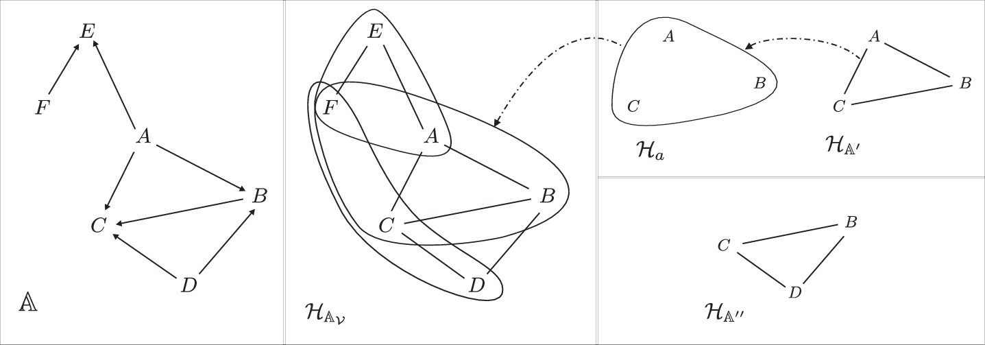
Consider the -structure whose vocabulary just contains the binary relation symbol , and such that . Such a simple one-binary-relation structure may be easily represented by the directed graph in the left part of Figure 1, where edge orientation reflects the position of the variables in . In this example, the associated hypergraph is just the undirected version of this graph. Let DM be a method that, on input , builds the -structure consisting of the seven base views of the form , for each tuple , plus the three relations , , and such that , , and . Figure 1 also reports .
A hypergraph is acyclic iff it has a join tree [3], i.e., a tree , whose vertices are the hyperedges of , such that if a node occurs in two hyperedges and of , then and are connected in , and occurs in each vertex on the unique path linking and in .
For two hypergraphs and , we write iff each hyperedge of is contained in at least one hyperedge of . Let . Then, a tree projection of with respect to is an acyclic hypergraph such that . Whenever such a hypergraph exists, we say that the pair has a tree projection (also, we say that has a tree projection w.r.t. ). The problem of deciding whether a pair of hypergraphs has a tree projection is called the tree projection problem, and it has recently been proven to be NP-complete [14].
Example 2
Consider again the setting of Example 1. It is immediate to check that the pair of hypergraphs does not have any tree projection. Consider instead the (hyper)graph reported on the right of Figure 1. The acyclic hypergraph is a tree projection of w.r.t. . In particular, note that the hyperedge “absorbs” the cycle in , and that is in its turn contained in the hyperedge .
Note that all the (known) structural decomposition methods can be recast as special cases of tree projections, since they just differ in how they define the set of views to be built for evaluating the CSP instance. For instance, a hypergraph has generalized hypertree width (resp., treewidth) at most if and only if there is a tree projection of w.r.t. (resp., w.r.t. ).
However, the setting of tree projections is more general than such traditional decomposition approaches, as it allows us to consider arbitrary sets of views, which often require more care and different techniques. As an example, we shall illustrate below that in the setting of tree projections it does not make sense to talk about “the” core of an -structure, because different isomorphic cores may differently behave with respect to the available views. This phenomenon does not occur, e.g., for generalized hypertree decompositions, where all combinations of constraints are available as views.
Example 3
Consider the structure illustrated in Example 1, and the structures and over the same vocabulary as , and such that and . The hypergraphs and are reported in Figure 1. Note that and are two (isomorphic) cores of , but they have completely different structural properties. Indeed, admits a tree projection (recall Example 2), while does not.
3.2 CSP Instances and tp-Coverings
We complete the picture of our unifying framework to deal with decomposition methods for constraint satisfaction problems, by illustrating some recent results in [15], which will be useful to our ends. Let us start by stating some preliminary definitions.
For a set of variables , let denote the structure with a fresh -ary relation symbol and domain , such that .
Definition 1
Let be a -structure. A set of variables is tp-covered in if there exists a core of such that has a tree projection.33 3 For the sake of completeness, note that we use here a core because we found it more convenient for the presentation and the proofs. However, it is straightforward to check that this notion can be equivalently stated in terms of any structure homomorphically equivalent to . The same holds for the related Definition 3.
For instance, it is easily seen that the variables are tp-covered in the -structure discussed in Example 1. In particular, note that the structure is associated with the same hypergraph that has a tree projection w.r.t. (cf. Example 3). Instead, the variables are not tp-covered in .
Given a CSP instance , we denote by the -structure that is obtained by enforcing generalized arc consistency on .
The following result, proved in [15] for a different setting, states the precise relationship between generalized-arc-consistent views and tp-covered sets of variables.
Theorem 3.2
Let be an -structure, and let be a -structure. The following are equivalent:
- (1)
A set of variables is tp-covered in ;
- (2)
For every -structure , for every -structure that is legal w.r.t. and , and for every relation with , .
Note that the result answered a long standing open question [10, 23] about the relationship between the existence of tree projections and (local and global) consistency properties in databases [15]. In words, the result states that just enforcing generalized arc consistency on the available views is a sound and complete procedure to solve ECSP instances if, and only if, we are interested in (projected) solutions over output variables that are tp-covered and occur together in some available view. Thus, in these cases, all solutions can be computed in polynomial time. The more general case where output variables are arbitrary (i.e., not necessarily included in some available view) is explored in the rest of this paper.
We now leave the section by noticing that as a consequence of Theorem 3.2, we can characterize the power of local-consistency for any decomposition method DM such that, for each pair , each view in contains the solutions of the subproblem encoded by the constraints over which it is defined. For the sake of simplicity, we state below the result specialized to the well-known decomposition methods and .
Theorem 2-bis. Let DM be a decomposition method in , let be an -structure, and let . The following are equivalent:
- (1)
A set of variables is tp-covered in ;
- (2)
For every -structure , and for every relation with , , where .
Proof (Sketch)
Preliminarily, it is easy to see that (2) in Theorem 3.2 may be equivalently stated as follows:
- (2’)
For every -structure , for every -structure that is legal w.r.t. and and such that , and for every relation with , .
The fact that trivially follows from Theorem 3.2. We have to show that holds as well. To this end, observe that if is not tp-covered in , by Theorem 3.2 (actually, ), we can conclude the existence of: (1) an -structure , (2) an -structure that is legal w.r.t. and and such that , and (3) a relation with such that (of course, by the legality of ). Consider now the -structure . Recall that each view in contains all the solutions of the subproblem encoded by the constraints over which it is defined. Since , it can be shown that each view in contains only solutions of the subproblem encoded by the constraints over which it is defined. Thus, for each relation , holds, which implies . The same line of reasoning applies to the tree decomposition method.
Note that if we consider decision problem instances () and the treewidth method (), from Theorem 2-bis, we (re-)obtain the nice characterization of [2] about the relationship between -local consistency and treewidth modulo homomorphic equivalence. If we consider generalized hypertree-width (), we get the answer to the corresponding open question for the unbounded arity case, that is, the precise power of the procedure enforcing -union (of constraints) consistency (i.e., the power of the algorithm for the decision problem described in [5]).
4 Enumerating Solutions of Output-Aware CSP Instances
The goal of this section is to study the problem of enumerating CSP solutions for classes of instances where possible output variables are part of the structure of the given instance. This is formalized by assuming that the relational structure contains domain constraints that specify the domains for such variables.
Definition 2
A variable is domain restricted in the -structure if there exists a unary distinguished (domain) relation symbol such that . The set of all domain restricted variables is denoted by .
We say that an ECSP instance is domain restricted if . Of course, if it is not, then one may easily build in linear time an equivalent domain-restricted ECSP instance where an additional fresh unary constraint is added for every output variable, whose values are taken from any constraint relation where that variable occurs. We say that such an instance is a domain-restricted version of .
Figure 2 shows an algorithm, named , that computes the solutions of a given ECSP instance. The algorithm is parametric w.r.t. any chosen decomposition method DM, and works as follows. Firstly, starts by transforming the instance into a domain restricted one, and by constructing the views in via DM. Then, it invokes the procedure . This procedure backtracks over the output variables : At each step , it tries to assign a value to from its domain view,44 4 With an abuse of notation, in the algorithm we denote by the base view in associated with the input constraint (in fact, no confusion may arise because the algorithm only works on views). and defines this value as the unique one available in that domain, in order to “propagate” such an assignment over all other views. This is accomplished by enforcing generalized arc-consistency each time the procedure is invoked. Eventually, whenever an assignment is computed for all the variables in , this solution is returned in output, and the algorithm proceeds by backtracking again trying different values.
Input: An ECSP instance , where ; Output: ; Method: update with any of its domain-restricted versions; let , ; invoke ; Procedure (: integer, : pair of structures, : integer, : tuple of values in ); begin 1. let ; 2. let ; 3. for each element do 4. if then 5. output ; 6. else 7. update with ; / is fixed to value / 8. ; end.
4.1 Tight Characterizations for the Correctness of
To characterize the correctness of , we need to define a structural property that is related to the one stated in Definition 1. Below, differently from Definition 1 where the set of output variables is treated as a whole, each variable in has to be tp-covered as a singleton set.
Definition 3
Let be an ECSP instance. We say that is tp-covered through DM if there is a core of such that has a tree projection.
Note that the above definition is purely structural, because (the right-hand structure) plays no role there. In fact, we next show that this definition captures classes of instances where is correct.
Theorem 4.1
Let DM be a decomposition method, let be an -structure, and let be a set of variables. Assume that is tp-covered through DM. Then, for every -structure , computes the set .
Proof (Sketch)
Let be any -structure. Preliminarily observe that if the original input instance, say , is tp-covered through DM, the same property is enjoyed by its equivalent domain-restricted version, say , computed in the starting phase of the algorithm. Thus, there is a core of such that has a tree projection, where . This entails that, , is tp-covered in . It is sufficient to show that, if , at the generic call of with as its first argument, is initialized at Step 2 with a non-empty set that contains all those values that may take, in any solution of extending the current partial solution ; otherwise (), , and the algorithm correctly terminates with an empty output without ever entering the for cycle. For the sake of presentation, we just prove what happens in the first call.The generalization to the generic case is then straightforward.
Let and assume that has been computed. From the tp-covered property of variables in and Theorem 3.2, it follows that , its domain view is such that . Thus, all values in the domain views associated with output variables occur in some solutions. This holds in particular for that is empty if, and only if, , in which case the cycle is skipped and the algorithm immediately halts with an empty output. Assume now that this is not the case, so that , and let be the chosen value at Step 3. Consider a new instance where the domain constraint for contains the one value . From the above discussion it follows that , and clearly the solutions of are all and only those of that extend the partial solution . Moreover, it is easy to check that the -structure obtained after the execution of Step 7 is legal w.r.t. , and recall that nothing is changed in the pair , which is (still) tp-covered through DM. Therefore, when we call recursively call at Step 8 with , we are in the same situation as in the first call, but going to enumerate the solutions of . At the end of this call, we just repeat this procedure with the next available value for , say , until all elements in have been considered (and propagated).
We now complete the picture by observing that Definition 3 also provides the necessary conditions for the correctness of . As in Theorem 2-bis, we state below the result specialized to the methods and .
Theorem 4.2
Let DM be a decomposition method in , let be an -structure, and let be a set of variables. Assume that, for every -structure , computes . Then, is tp-covered through DM.
Proof (Sketch)
Assume that is not tp-covered through DM, and let be a maximal set of output variables such that is tp-covered through DM. In the case where , there is no core of such that has a tree projection. Thus, we can apply Theorem 2-bis and conclude that there are an -structure , and a relation such that has a solution while is empty, with . It follows that will not produce any output. Consider now the case where , and where any is a variable such that is not tp-covered through DM. Let be the relational structure , which is such that has a tree projection. Then, is not tp-covered in . By Theorem 2-bis, there are an -structure , and a relation with such that , where . In fact, we can show that such a “counterexample” structure can be chosen in such a way that there are (full) solutions for the problem having the following property: some values in belongs to the generalized arc consistent structure where variables in are fixed according to . Thus while enumerating such a solution , generates wrong extensions of this solution to the variable .
4.2 Tight Characterizations for Enumerating Solutions with Polynomial Delay
We next analyze the complexity of .
Theorem 4.3
Let be an -structure, and be a set of variables. If is tp-covered through DM, then runs WPD.
Proof
Assume that is tp-covered through DM. By Theorem 4.1, we know that computes the set . Thus, if the algorithm does not output any tuple, we can immediately conclude that the ECSP instance does not have solutions. Concerning the running time, we preliminary notice that the initialization steps are feasible in polynomial time. In particular, computing and is feasible in polynomial time, by the properties of the decomposition method DM (see Section 3). To characterize the complexity of the recursive invocations of , we have to consider instead two cases.
In the case where there is no solution, we claim that the -structure obtained by enforcing generalized arc consistency in the first invocation of (i.e., for ) is empty. Indeed, since is tp-covered through DM, then is tp-covered in —just compare Definition 1 and Definition 3. It follows that we can apply Theorem 3.2 on the set in order to conclude that, for every relation with , . Since, is empty, the above implies that is empty too. Thus, invokes just once , where the only operation carried out is to enforce generalized arc consistency, which is feasible in polynomial time.
Consider now the case where is not empty. Then, the first solution is computed after recursive calls of the procedure , where the dominant operation is to enforce generalized arc consistency on the current pair . In particular, by the arguments in the proof of Theorem 4.1, it follows that does not have to backtrack to find this solution: after enforcing generalized arc consistency at step , any active value for is guaranteed to occur in a solution with the current fixed values for the previous variables , . Since can be enforced in polynomial time, this solution can be computed in polynomial time as well.
To complete the proof, observe now that any solution is provided in output when is invoked for . After returning a tuple of values , may need to backtrack to a certain index having some further (different) value to be processed, fix with this value, propagate this assignment, and continue by processing variable . Thus, at most invocations of are needed to compute the next solution, and no backtracking step may occur before we found it. Therefore, runs WPD.
By the above theorem and the definition of domain restricted variables, the following can easily be established.
Corollary 1
Let be any class of -structures such that, for each , is tp-covered through DM. Then, for every -structure , and for every set of variables , the ECSP instance is solvable WPD.
In the case of bounded arity structures and if the (hyper)tree width is the chosen decomposition method, it is not hard to see that the result in Corollary 1 is essentially tight. Indeed, the implication in the theorem below easily follows from the well-known dichotomy for the decision version [17], which is obtained in the special case of ECSP instances without output variables ().
Theorem 4.4
Assume . Let be any class of -structures of bounded arity. Then, the following are equivalent:
- (1)
has bounded treewdith modulo homomorphic equivalence;
- (2)
For every , for every -structure , and for every set of variables , the ECSP instance is solvable WPD.
Actually, from an application perspective of this result, we observe that there is no efficient algorithm for the no-promise problem for such classes. In fact, the following proposition formalizes and generalizes previous observations from different authors about the impossibility of actually trusting positive answers in the (promise) decision problem [24, 4].
We say that a pair is a certified projected solution of if, by using the certificate , one may check in polynomial-time (w.r.t. the size of ) whether . E.g., any full solution extending is clearly such a certificate. If , is also empty, and is intended to be a certificate that is a “Yes” instance of the decision CSP. Finally, we assume that the empty output is always a certified answer, in that it entails that the input is a “No” instance, without the need for an explicit certificate of this property.
Proposition 1
The following problem is NP-hard: Given any ECSP instance , compute a certified solution in , whenever is tp-covered through DM; otherwise, there are no requirements and any output is acceptable. Hardness holds even if DM is the treewidth method with , the vocabulary contains just one binary relation symbol, and .
Proof
We show a polynomial-time Turing reduction from the NP-hard 3-colorability problem. Let be a Turing transducer that solves the problem, that is, whenever is tp-covered through DM, at the end of a computation on a given input its output tape contains a certified solution in , otherwise, everything is acceptable. In particular, we do not pretend that recognizes whether the above condition is fulfilled.
Then, we use as an oracle procedure within a polynomial time algorithm that solves the 3-colorability problem. Let be any given graph, and assume w.l.o.g. that it contains a triangle , , and . (Otherwise, select any arbitrary vertex of and connect it to two fresh vertices and , also connected to each other. It is easy to check that this new graph is 3-colorable if, and only if, the original graph is 3-colorable, as the two fresh vertices have no connections with the rest of the graph.) Build the (classical) binary CSP where the vocabulary contains one relation symbol , and the set of variables is . Moreover, , and . Consider the treewidth method for , and compute in polynomial time the pair where and . In particular, observe that the hypergraph contains a hyperedge for every triple of vertices of .
It is well-known and easy to see that is 3-colorable if, and only if, , that is, if there is a homomorphism from to a triangle (indeed, is a triangle). Therefore, if is 3-colorable, the triangle substructure such that is homomorphically equivalent to . Moreover, in this case the hypergraph consisting of the single hyperedge is a tree projection of w.r.t. , or, equivalently, the treewidth of is .
Now, run on input and consider its first output certificate —say, for the sake of presentation, a full solution for the problem. Then check in polynomial time whether is a legal certificate—in our exemplification, whether it encodes a solution of the given instance. If this is the case, we know that is 3-colorable; otherwise, we conclude that is not 3-colorable. Indeed, must be correct on 3-colorable graphs, because there exists a tree projection of (and thus of any core of —note that and thus there is no further requirement) w.r.t. . Since all these steps are feasible in polynomial-time, we are done.
5 Enumerating Solutions over Arbitrary Output Variables
In this section we consider structural properties that are independent of output variables, so that tractability must hold for any desired sets of output variables. For this case, we are able to provide certified solutions WPD, which seems the more interesting notion of tractability for actual applications.
Input: An ECSP instance , where ; Output: for each solution , a certified solution ; Method: let be the variables of ; update with any of its domain restricted versions; let , ; invoke ; Procedure (: integer, : pair of structures, : integer, : tuple of values in ); begin 1. let ; 2. if and is empty then output “DM failure” and Halt; 3. let ; 4. for each element do 5. if then 6. output the certified solution ; 7. else 8. update with ; / is fixed to value / 9. ; 10. if then Break; end.
Figure 3 shows the algorithm computing all solutions of an ECSP instance, with a certificate for each of them. The algorithm is parametric w.r.t. any chosen decomposition method DM, and resembles in its structure the algorithm. The main difference is that, after having found an assignment for the variables in , still iterates over the remaining variables in order to find a certificate for that projected solution. Of course, does not backtrack over the possible values to be assigned to the variables in , since just one extension suffices to certify that this partial solution can be extended to a full one. Thus, we break the cycle after an element is picked from its domain and correctly propagated, for each , so that in these cases we eventually backtrack directly to (to look for a new projected solution).
Note that incrementally outputs various solutions, but it halts the computation if the current -structure becomes empty. As an important property of the algorithm, even when this abnormal exit condition occurs, we are guaranteed that all the elements provided as output until this event are indeed solutions. Moreover, if no abnormal termination occurs, then we are guaranteed that all solutions will actually be computed. Correctness follows easily from the same arguments used for , by observing that, whenever has a tree projection, the full set of variables is tp-covered through DM.
Theorem 5.1
Let be an -structure, and be a set of variables. Then, for every -structure , computes WPD a subset of the solutions in , with a certificate for each of them. Moreover,
- •
If outputs “DM failure”, then does not have a tree projection;
- •
otherwise, computes WPD .
Moreover, we next give some evidence that, for bounded arity classes of instances, we cannot do better than this. In particular, having bounded width tree-decompositions of the full structure seems a necessary condition for the tractability of the enumeration problem WPD w.r.t. arbitrary sets of output variables (and for every -structure).

The main gadget of the proof that tree-decompositions are necessary for tractability is based on a nice feature of grids. Figure 4 shows the basic idea for the simplest case of a relational structure with only one relation symbol such that is (the edge set of) an undirected grid. Then, any substructure of where contains just one tuple is a core of . However, if we consider the variant of where there is a domain constraint for every corner of the grid (depicted with the circles in the figure), then the unique core is the whole structure. In fact, we next prove that this property holds for any relational structure whose Gaifman graph is a grid.
Lemma 1
Let be an -structure whose Gaifman graph is a grid . Moreover, let be the set of its four corners, and assume they are domain restricted, i.e., . Then, is a core.
Proof
Let be such a grid, and consider any homomorphism that maps to any of its substructures . Since the four corners are domain restricted, must hold for each of them (as is the one tuple of its domain constraint ). We say that such elements are fixed.
Consider the first row of . We have seen that its endpoints, which are grid-corners, are fixed. It is easy to check that cannot map the path to any path that is longer than . However, is the shortest path connecting the fixed endpoints and , and hence it must be mapped to itself. That is, for every element occurring in , and thus, by the same reasoning, for every element occurring in the last row, and in the first and the last columns of the grid. It follows that the endpoints and of the second row are fixed as well, and we may apply the same argument to show that all elements occurring in are fixed, too. Eventually, row after row, we get that all elements of are fixed, and thus the identity mapping is the only possible endomorphism for , which entails that is a core.
We also exploit the grid-based construction from [17], whose properties relevant to this paper may be summarized as follows.
Proposition 2 ([17])
Let and , and let be any -structure such that the -grid is a minor of the Gaifman graph of a core of . For any given graph , one can compute in polynomial time (w.r.t. ) a -structure such that contains a -clique if, and only if, there is a homomorphism from to .
We can now prove the necessity of bounded treewidth for tractability WPD.
Theorem 5.2
Assume . Let be any bounded-arity recursively-enumerable class of -structures closed under taking minors. Then, the following are equivalent:
- (1)
has bounded treewdith;
- (2)
For every , for every -structure , and for every set of variables , the ECSP instance is solvable WPD.
Proof
The fact that holds follows by specializing Theorem 5.1 to the tree decomposition method. We next focus on showing that also holds.
Let be such a bounded-arity class of -structures closed under taking minors, and having unbounded treewidth. From this latter property, by the Excluded Grid Theorem [22] it follows that every grid is a minor of the Gaifman graph of some -structure in . Moreover, because this class is closed under taking minors, every grid is actually the Gaifman graph of some -structure in .
Assume there is a deterministic Turing machine that is able to solve with polynomial delay any ECSP instance such that . We show that this entails the existence of an FPT algorithm to solve the -hard problem -Clique, which of course implies .
Let be a graph instance of the -Clique problem, with the fixed parameter . We have to decide whether has a clique of cardinality . We enumerate the recursively enumerable class until we eventually find an -structure whose Gaifman graph is the -grid. Let be its vocabulary. Note that searching for this structure depends on the fixed parameter only (in particular, it is independent of ).
Let be the variables at the four corners of this grid, and let be the extension of such that, for every variable , the vocabulary of contains the domain relation-symbol . Thus, the Gaifman graph of is the same -grid as for , but its four corners are domain-restricted in (). From Lemma 1, is a core.
Recall now the grid-based construction in Proposition 2: We can build in polynomial time (w.r.t. ) a structure such that there is a homomorphism from to if, and only if, has a clique of cardinality .
Consider the ECSP instance where by construction, and is the restriction of to the vocabulary . Thus, compared with , the -structure may miss the domain constraint for some output variable . It is easy to see that is a homomorphism from to if, and only if, is a homomorphism from to such that, for every , . Therefore, to decide whether such a homomorphism exists (and hence to solve the clique problem), we can just enumerate WPD the set of solutions and check whether the four domain constraints on the corners of are satisfied by any of these solutions. Now, recall that is built in polynomial time from , and thus every variable may take only a polynomial number of values, and of course all combinations of four values from , , are polynomially many. It follows that actually takes polynomial time for computing , and one may then check in polynomial time whether the additional domain constraints in are satisfied or not by some solution in .
By combining the above ingredients, we got an FPT algorithm to decide whether has a clique of cardinality .
References
- [1] I. Adler. Tree-Related Widths of Graphs and Hypergraphs. SIAM Journal Discrete Mathematics, 22(1), pp. 102–123, 2008.
- [2] A. Atserias, A. Bulatov, and V. Dalmau. On the Power of k-Consistency, In Proc. of ICALP’07, pp. 279–290, 2007.
- [3] P.A. Bernstein and N. Goodman. The power of natural semijoins. SIAM Journal on Computing, 10(4), pp. 751–771, 1981.
- [4] A. Bulatov, V. Dalmau, M. Grohe, and D. Marx. Enumerating Homomorphism. In Proc. of STACS’09, pp. 231–242, 2009.
- [5] H. Chen and V. Dalmau. Beyond Hypertree Width: Decomposition Methods Without Decompositions. In Proc. of CP’05, pp. 167–181, 2005.
- [6] D. Cohen, P. Jeavons, and M. Gyssens. A unified theory of structural tractability for constraint satisfaction problems. Journal of Computer and System Sciences, 74(5): 721-743, 2008.
- [7] D.A. Cohen. Tractable Decision for a Constraint Language Implies Tractable Search. Constraints, 9(3), 219–229, 2004.
- [8] R. Dechter and A. Itai. Finding All Solutions if You can Find One. In Proc. of AAAI-92 Workshop on Tractable Reasoning, pp. 35–39, 1992.
- [9] R.G. Downey and M.R. Fellows. Parameterized Complexity. Springer, New York, 1999.
- [10] N. Goodman and O. Shmueli. The tree projection theorem and relational query processing. Journal of Computer and System Sciences, 29(3), pp. 767–786, 1984.
- [11] G. Gottlob, N. Leone, and F. Scarcello. A Comparison of Structural CSP Decomposition Methods. Artificial Intelligence, 124(2): 243–282, 2000.
- [12] G. Gottlob, N. Leone, and F. Scarcello. Hypertree decompositions and tractable queries. Journal of Computer and System Sciences, 64(3), pp. 579–627, 2002.
- [13] G. Gottlob, N. Leone, and F. Scarcello. Robbers, marshals, and guards: game theoretic and logical characterizations of hypertree width. J. of Computer and System Sciences, 66(4), pp. 775–808, 2003.
- [14] G. Gottlob, Z. Miklós, and T. Schwentick. Generalized hypertree decompositions: NP-hardness and tractable variants. Journal of the ACM, 56(6), 2009.
- [15] G. Greco and F. Scarcello. The Power of Tree Projections: Local Consistency, Greedy Algorithms, and Larger Islands of Tractability. To appear in Proc. of PODS’10.
- [16] M. Grohe, T. Schwentick, and L. Segoufin. When is the evaluation of conjunctive queries tractable? In Proc. of STOC’01, pp. 657–666, 2001.
- [17] M. Grohe. The complexity of homomorphism and constraint satisfaction problems seen from the other side. Journal of the ACM, 54(1), 2007.
- [18] M. Grohe and D. Marx. Constraint solving via fractional edge covers. In Proc. of SODA’06, pp. 289–298, 2006.
- [19] D. Marx. Approximating fractional hypertree width. In Proc. of SODA’09, pp. 902–911, 2008.
- [20] D. Marx. Tractable Hypergraph Properties for Constraint Satisfaction and Conjunctive Queries. To appear in Proc. of STOC’10.
- [21] N. Robertson and P.D. Seymour. Graph minors III: Planar tree-width. Journal of Combinatorial Theory, Series B, 36, pp. 49-64, 1984.
- [22] N. Robertson and P.D. Seymour. Graph minors V: Excluding a planar graph. Journal of Combinatorial Theory, Series B, 41, pp. 92-114, 1986.
- [23] Y. Sagiv and O Shmueli. Solving Queries by Tree Projections. ACM Transaction on Database Systems, 18(3), pp. 487–511, 1993.
- [24] F. Scarcello, G. Gottlob, and G. Greco. Uniform Constraint Satisfaction Problems and Database Theory. In Complexity of Constraints, LNCS 5250, pp. 156–195, Springer-Verlag, 2008.